Above ground biomass carbon assessment using field, satellite data and model based integrated approach to predict the carbon sequestration potential of major land use sector of Arunachal Himalaya, India

Abstract

The land-use sector needs special importance owing to its ability to store and emit carbon back to the atmosphere. Land-use changes and their correlations could elucidate conditions that put forests at risk of conversion to other land uses. The impact of rapid forest cover change tends to reduce the percentage of forest cover, thereby reducing the potential for carbon storage in woody biomass. The study was conducted in the state of Arunachal Pradesh to estimate the above-ground biomass, carbon pool and sequestration potential of major land-use sectors. The above-ground biomass of selected land-uses viz. dense forest, moderately dense forest, open forest, plantations, Jhum >5 years, Jhum <5 years and current jhum are 332.28 t ha⁻¹, 246.63 t ha⁻¹, 145.36 t ha⁻¹, 179.31 t ha⁻¹, 149.63 t ha⁻¹, 55.40 t ha⁻¹, 16.84 t ha⁻¹ respectively. The developed model is derived from Soil Adjusted Vegetation Index (SAVI) and Atmospherically Resistant Vegetation Index (ARVI) for prediction of above-ground biomass (AGB) (R² = 0.85, p < 0.05). The resultant R² value of 85% predicts that 79% of accuracy could be assumed by the model. The RMSE of the model was 53.21 t ha⁻¹, having no multicollinearity problem keeping tolerance (0.49) and VIF (2.80). The spatial AGB density map was predicted using a step-wise linear regression model which used AGB, SAVI and ARVI of the corresponding sample plot location. The implication of the land-use change revealed that about 84% carbon will be lost from dense forest once it is converted to Jhum (Jhum is the alternate name of Shifting cultivation in India) followed by Jhum <5 years (65%). It is pertinent to mention here that, the present analysis will help the policymakers in visualizing a proper developmental goal to regulate land-use changes for achieving the higher carbon stock and maintaining balance in the global climate scenario.

Keywords:

• Biomass
• carbon stock
• land-use change
• Northeast India
• vegetation indices

Introduction

Rapid urbanization and forest clearing deteriorate forest ecosystem and adversely affect the microclimate, regeneration, soil dynamics and enhance the emission of greenhouse gases. Current land-use practices by the population for their sustenance of developing countries have enormous effects on the forest carbon accumulation and storage. Due to large human interference, the forest degradation and deforestation in tropical and subtropical forests are recognized as a key contributor to global greenhouse gas emission [1]. The scale of land-use transition has significantly transformed the forest ecosystem’s physico-chemical and biological processes [2]. Land conversion has been recognized as the main driver which immensely influences the earth’s ecosystem and climate [3]. The land-use changes alone prompted about 12.5% of CO₂ emissions from 1990 to 2010 [4]. The terrestrial ecosystems act as the foremost source of carbon sinks and have been discussed at the desired pace [5]. The IPCC [6] highlighted the main carbon accumulation and sequestration ensues in above- and below ground of the forest ecosystem. Plant standing biomass, understory vegetation, litter and soil organic carbon conjointly contribute to the major carbon pool.

The aboveground biomass (AGB) of the forest has contributed much towards carbon storage and is being directly impacted by the land-use change. Pan et al. [7] reported that the average amount of 4.1 Pg C/year of global carbon concentration in these two pools from 2000 to 2007, although this rate narrowed by the carbon released through the tree felling. They also stated that about 2.8 Pg C/year of carbon is released due to forest alteration. The IPCC [6] described the disastrous impacts of GHGs emissions around the world and the agencies like the Kyoto Protocol and the Paris Agreement came forward and made policies to control the GHGs emission. Further, enhancing the forest ecosystem’s carbon sequestration through afforestation and refining forest management were recognized as key climate policies for reducing such emissions. The carbon sequestration promises to mitigate the climate targets that depend on the carbon sink size enhancement and fossil fuel reduction [8]. The AGB has been recognized as a vital indicator of forest vegetation growth and its health [9, 10]. The precise estimation of anthropogenic induced CO₂ emission having very perplexing issues reflects in the process of decision making. Hence, researchers tried every possible way for precise estimation of biomass stock and carbon sequestration to minimize the challenges related to CO₂ emission. Therefore, accurate AGB estimation and stock assessment at different levels are of utmost importance to the decision-makers for national planning [11]. The biomass and carbon stock have been done by various methods and approaches based on forest inventory data which is more precise among all available techniques [12]. The non-destructive sampling approach in conjunction with various models such as the forest yield model and remote sensing approaches were preferred for the biomass and carbon stock assessment [13]. The remote sensing approach includes optical and microwave data having great advantages viz. accessibility to the inaccessible area, repetitive aerial coverage and availability of historical datasets with cost-effectiveness data for assessing the vegetation conditions [14]. Recently, researchers have used different satellite data such as NOAA AVHRR [15], MODIS [16], IKONOS [17], WorldView-2 [18], Resourcesat-2 [19], Landsat OLI [20, 21] for AGB and carbon estimation at minimal cost with acceptable precision. It uses spectral reflectance properties of the satellite data as these contained an integrated effect of forest canopy through the factors like vegetation composition, soil characteristics, atmospheric condition and topographic effect [22].

Many researchers have widely used the spectral vegetation indices (VI) model for estimating the biomass [20, 22–26] in different parts of the country and worldwide. The data availability of biomass using advanced models on carbon sequestration by the woody biomass is still limited in the state. Thus, improved quantification is important for understanding the contribution and potential of land uses. The present study aims to estimate and predict the biomass, carbon stock and sequestration in different land-use sectors of Arunachal Pradesh, Northeast India and intend future trend of carbon stock through spatial modeling. It also briefly describes the current scenario of carbon stock in the study area using forest-based data and relating plot-based results in pixel-based information of optical remote sensing to predict landscape-level carbon stock.

Materials and methods

Study area

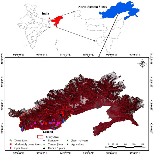
The state of Arunachal Pradesh is the easternmost state of India and is known as the “land of the rising sun” in reference to its position. It is situated between 26°28′ N to 29°30′ N latitude and 91°30′ E to 97°30′ E longitude, with Itanagar as the capital of the state having a geographical area of 84,000 km² (http://www.arunachalpradesh.gov.in/) (Figure 1). It borders with the state of Assam to the south and Nagaland to the southeast. Myanmar lies towards the east, Bhutan towards the west, and Tibet to the north. The state is blessed with extraordinary diversity and divided into two major physiographic regions i.e. Arunachal Himalayas and the Brahmaputra valley. The state shows great variability in altitudinal variation (78 m asl to >2500 m asl) and is grouped into four major agro-climatic regions i.e. tropical, subtropical, temperate and alpine. Spatial distribution and area coverage results reveal that the alpine zones cover about 25,792 km² followed by subtropical zones (24,656 km²), temperate zones (19,277 km²) and tropical zones (12,397 km²). The climate of the state varies sharply with changes in its latitude and elevation. The areas at very high elevation in the upper Himalayas close to the Tibetan border enjoy an alpine climate while below this region is mostly temperate. The areas at the Sub-Himalayan experiences a humid subtropical climate along with hot summers and mild winters. The average mean maximum and minimum temperature vary between 29.5 °C and 17.7 °C in subtropical regions. It is on a scale of 21.4 °C and 2.4 °C in cold humid regions and the foothills. But the plains experience higher temperatures. The Land use/cover map of the study area has been generated using Landsat OLI satellite data (2016). Accordingly, four districts namely Papum Pare, Lower Subansiri, East Kameng and West Kameng were selected for study keeping the feasibility and accessibility of major land-use sectors. Following the above, permanent plots were laid (Figure 1).

Figure 1. Map showing state of Arunachal Pradesh, Northeast India and permanent plots.

Methods

Satellite data acquisition

The precision of spatial data is important for the user and is essential in the evaluation of the quality of the results of data processing. Landsat OLI optical remote sensing data sets and ASTER elevation data sets of 2016 were used for the study (Table 1) which were downloaded from Earth Explorer (https://earthexplorer.usgs.gov), a public domain of NASA. The cloud-free images were selected and red, green, blue and NIR bands were included in the analysis. All the images were georeferenced to the common UTM (Universal Transversal Mercator) projection with WGS 84 datum (Zone 46). The images were converted to top of atmospheric (TOA) reflectance by radiometric correction method as per Landsat8 user handbook. As the study area covers the complex terrain with dense forest cover, it is a prerequisite to removing the topographic illumination effect from all the images. Hence, the improved cosine correction method Civco [27] was applied to all images. For the topographic correction of satellite imageries, we have used the ATCORE tool of ERDAS Imagine 2014 software [28]. The ASTER DEM data with a 30 m resolution was used for topographic correction. The DEM images were re-sampled to Landsat OLI pixel size by the nearest neighborhood transformation [29]. For the forest inventory process, an unsupervised classification approach was done.

Table 1. Landsat 8 OLI data characteristics.

Data used	Path/row	Data acquisition month	Wavelength of the band (μm)	Spatial resolution (M)	Swath (km)
Landsat 8 OLI	133/ 40, 134/40, 134/41, 135/40, 135/41, 136/40, 136/41, 137/41	Nov 2016 Jan, 2018	Band 2 – Blue (0.45 - 0.51)	30	185
			Band 3 – Green (0.53 - 0.59)
			Band 4 – Red (0.64 - 0.67)
			Band 5 - Near Infrared (NIR) (0.85–0.88)

Forest inventory data collection

Keeping major agro-climatic zones, altitudinal gradients and cover into consideration, permanent plots were selected and demarcated for the detailed study. Classified land use map shows mixed forests, plantations and abandoned or degraded forest among the major land-use sectors in major agro-climatic zones. In each of the zones and major land-use sectors, sampling plots were randomly selected in replicates. Forest inventory data were collected for a period of two years (2016–2017) and altogether 127 permanent plots were studied. Among these, 78, 18, 15 and 16 plots belong to forest, plantation, Jhum and paddy cultivation, respectively. Each plot size was 31.6 m × 31.6 m for trees or woody species (>30 cm GBH), sub-plot sized 5 m × 5 m for shrubs/saplings (<30 cm GBH and >1 m height) and sub-plot sized 1 m × 1 m for seedlings/herbs (>1 m height) for biomass enumeration. Coordinates of each plot were recorded by using the global position system (GPS). In each plot, the height of the tree and girth at breast height (GBH) of each individual was measured using a clinometer and measuring tape, respectively. Based on the GBH and height, the plot based AGB was calculated for trees having girth ≥30 cm at girth breast height (1.37 m) by applying a general allometric equation for the northeastern region of India proposed by Nath et al. [30] which is based on stem diameter, height and wood density of the species. For shrub and herb species destructive approach is adopted in the current study. For shrub species, all the species present in the 5 m × 5 m sub-plot was recorded. One to two individuals of different species were cut, and their fresh weights were taken. Then the species were brought to the laboratory for dry weight measurement. The average dry weight of the individual species was multiplied by the number of the same species to estimate the AGB of the species. Similarly, for the herbaceous species, all plant species present in the 1 m × 1 m sub-plot were harvested and brought to the laboratory for estimating the dry weight of herbaceous species.

Vegetation indices and modeling of AGB

The Landsat OLI vegetation indices include difference vegetation index (DVI) which is a simple difference between near-infrared (NIR) and red (R) band ratio, normalized difference vegetation index (NDVI) which is the ratio of NIR and R bands, atmospheric resistant vegetation index (ARVI) which uses three-band ratio to minimize the atmospheric scattering effect. Soil adjusted vegetation index (SAVI) minimizes soil brightness effects in the satellite image and enhanced vegetation index (EVI) is a complex index and high sensitivity to high AGB region as it eliminates the aerosol influence and canopy background effect. Hence, these vegetation indices (Table 2) were incorporated to analyze the best relationship between the AGB and vegetation indices. For plot-wise vegetation indices derivation, at first, the coordinates of each plot laid upon different VI images and VI values were extracted by using a tool that extracts by point values in ArcGIS software.

Table 2. Vegetation indices used for correlation analysis for spatial mapping of biomass and carbon.

Vegetation Indices	Expression	Author
DVI	DVI = NIR − R	Richardson and Wiegand [31]
NDVI	NDVI = (NIR − R)/(NIR + R)	Rouse et al. [32]
SAVI	SAVI = [(NIR − R)/(NIR + R + L)](1 + L) Where L = 0.5 for intermediated vegetation cover	Huete [33]
ARVI	ARVI = (NIR − RB)/(NIR + RB)	Kaufmann and Tanre, [34]
EVI	EVI = G * (NIR − R)/(NIR + C1R − C2B + L) Where: C1 = 6; C2 = 7.5; L = 1; G = 2.5	Liu and Huete, [35]

DVI: Difference vegetation index, NDVI: Normalized difference vegetation index, SAVI: Soil adjusted vegetation index, ARVI: Atmospheric resistant vegetation index, EVI: Enhanced vegetation index.

Out of 127 sample data, a total of 111sample data belong to forest, plantations and Jhum fields; and are used to derive the relationship between plot AGB and VIs which is a prerequisite for modeling of AGB for the study region. Some researchers have applied linear regression approach [36, 37], multi-regression approach [18, 38, 39], non-linear regression [40], non-parametric model [41], artificial neural network [42, 43]. In the present study, a linear regression analysis has been applied by step-wise multi-linear regression analysis for assessing the relationship between AGB and vegetation indices. The pixel values of different indices were extracted for each plot of the major land-use sector by coordinates of the plot in ArcGIS 10.3. The extracted different VIs was evaluated based on Pearson correlation (r) and Coefficient of determination (R²), Root Mean Square Error (RMSE), and p level was applied. The VIs with high r and R² indicated the best fit for AGB modeling. Here the AGB modeling was done by applying the multi-linear regression approach using origin 7 software (https://www.originlab.com/). The multi-linear regression approaches some time subjected to multicollinearity and overfitting difficulties in the analysis which may pose a serious problem in modeling. Hence, to overcome this and to confirm the reliability of the model, R², RMSE, multicollinearity of variables, tolerance (Tolerance = 1 − R_x²), and variance inflation factor {VIF = VIFj= 1/(1 − R_j²)} were determined. To indicate a multicollinearity problem, a tolerance limit below 0.10 [39, 44], VIF value greater than 10 [38, 39] were determined. From each land-use type, 75% of AGB data were randomly selected for the AGB modeling equation, whereas the remaining 25% of AGB data for validation of the model.

Mapping carbon density and sequestration using CO₂ fix model

The spatial AGB stock density map was predicted for the state using resultant modeled AGB stock data derived from stepwise linear regression analysis, and subsequently, a map was prepared in the GIS environment. Further, a carbon density map was also prepared by taking a fraction of 55% of AGB [45]. Spatial carbon modeling was done using CO₂FIX empirical model, which is a stand-level simulation model that quantifies the C stock in the forests and soil [46]. The model has multiple cohorts, which allows the researchers to incorporate the growth data for different land-use types. It also has different submodules like growth by stand density, intercohort competition, the harvested process, and soil dynamics, etc. [47]. This model has been used to estimate the C stock over a while in a variety of ecosystems around the globe. To run this model forest inventory data were used. The difference data of AGBC 2016 and 2018 were used in terms of gain or loss in carbon stock for the future projection of spatial carbon density or carbon sequestration in the study area.

Results

Floristic composition

The number of trees recorded from the field inventory of 111 (11.1 ha) sample plots were 5948. Of the total trees recorded, 1538 number of trees were recorded from dense forests (DF), 1212 trees from moderately dense forests(MDF), 1659 trees from open forests(OF), 995 trees from plantations (PL), 50 trees from current hum (CJH), 138 trees from Jhum less than 5 years(JH < 5), and 712 trees from >5 years Jhum fields(JH > 5). The study recorded 159 woody (>30 cm GBH) species from dense forests followed by open forests (121 species), moderately dense forests (105 species), plantations (51 species), Jhum >5 years (31 species), Jhum <5 years having 24 species and lowest in current Jhum (19 species) fields. Maximum stand density (individuals/ha) was recorded in Jhum land > 5 years, followed by open forest, dense forest, moderately dense forest, plantations, Jhum <5years and current Jhum fields. However, the maximum diversity index was recorded for forest land followed by plantations and minimum in the current Jhum field. On the contrary, the Simpson dominance index followed a reverse trend in results to that of the diversity index. The tree density and basal area of the study region varied considerably among the land-use sectors and the values ranged between 100 and 712 stems ha⁻¹, with maximum stand density (712 stem ha⁻¹) in >10 years Jhum fields followed by open forests, dense forests, plantations, moderately dense forests and Jhum fields. The maximum basal area was recorded in forests and plantations than the Jhum fields despite low stand density mainly due to the presence of the large number of individuals having more girth (Table 3).

Table 3. Community characteristics of the major land use sectors.

Parameters	Major landuse sectors
	DF	MDF	OF	PL	CJH	JH_5	JH
Woody individual	1538	1212	1659	995	50	138	356
Number of species	159	105	120	51	19	24	31
Area surveyed (ha)	2.7	2.2	2.9	1.8	0.5	0.5	0.5
Stand density (stem/ha)	570	550	572	553	100	276	712
Basal area (m^2/ha)	54.26	41.16	22.46	36.42	2.57	9.13	25.8
Simpson dominance index	0.01	0.02	0.02	0.06	0.07	0.05	0.08
Shannon diversity index	4.66	4.26	4.32	3.37	2.65	3.52	3.03

DF: Dense forest, MDF: Moderately dense forest, OF: Open forest, PL: Plantation, JH > 5: Jhum > 5 years, JH < 5: Jhum < 5 years, CJH: Current jhum.

Aboveground biomass and carbon stock

The AGB of selected land-use was ranged between 16.84 and 332.28 t ha⁻¹. Among the land use, dense forest possessed maximum AGB (332.28 t ha⁻¹) followed by moderately dense forest, plantation and open forest. In the abandoned Jhum fields of varying ages, the maximum AGB was recorded as 149.63 t ha⁻¹ for Jhum fields having >5 years followed by Jhum field with < 5 years and current Jhum fields. The AGB for shrubs/saplings of dense forests possessed a maximum value of 25.27 t ha⁻¹ followed by moderately dense forests, plantations, open forests, Jhum fields having >5 years,< 5 years and current Jhum. AGB contribution by the herbs/seedlings, open forests recoded maximum AGB of 4.22 t ha⁻¹ and least in moderately dense forests. In Jhum fields, the maximum biomass contribution was observed for Jhum fields of old ages (Table 4). Girth-class density distribution indicates that girth class (<90 cm GBH) constitutes 22–62% of the total number of stems in different land-use sectors but it contributed only 7–59% of total biomass. However, individuals having a girth >90 cm GBH were comparatively lesser in number than former girth-class but have contributed more towards basal area and biomass. Higher biomass contribution was recorded for trees having girth (91–120 cm GBH) followed by trees having girth (>180 cm GBH) in all the forest types despite low stand density (Figure 2).

Figure 2. Girth wise density and AGB distribution of major landuse sectors.

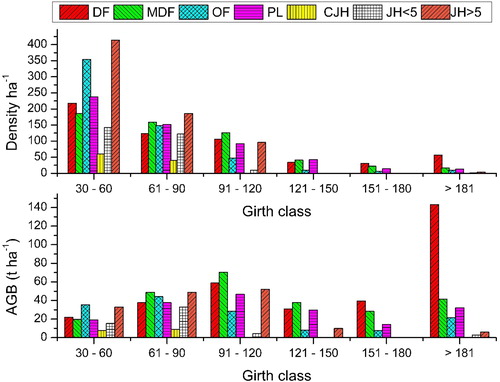
Table 4. Component wise biomass contribution in major landuse sectors of Arunachal Pradesh.

Landuse sectors	AGB	BGB	Herbs/seedlings	Shrubs/saplings	Total biomass
DF	332.28	89.71	4.18	25.27	451.44
MDF	246.63	71.52	3.89	23.85	345.89
OF	145.36	42.15	4.22	14.42	206.15
PL	179.31	52.00	4.1	23.13	258.54
JH > 5	149.63	43.39	3.13	7.27	203.42
JH < 5	55.40	16.06	2.13	4.11	77.70
CJH	16.84	4.88	2.25	3.83	27.8

DF: Dense forest, MDF: Moderately dense forest, OF: Open forest, PL: Plantation, JH > 5: Jhum > 5 years, JH < 5: Jhum < 5 years, CJH: Current jhum.

Modeling relationship between VI and field AGB

The linear regression analysis of various vegetation indices and plot-wise AGB was derived and shown in Table 5. The Pearson’s r values of VIs ranged from 0.52 to 0.90 and R² varied between 0.32 to 0.81. All the VIs showed a significant and positive correlation with AGB. However, ARVI (r = 0.90, R² = 0.81) was the best VI among the selected indices followed by the SAVI, EVI, NDVI and DVI. Based on the stepwise linear multiple regression approach, the model for AGB estimation for the study region has been expressed as follows: $$\mathrm{AGB}=93.65\mathrm{*}\mathrm{SAVI}+88.79\mathrm{*}\mathrm{ARVI}-36.17$$

Table 5. Linear regression between vegetation indices (VIs) and Plot based AGB.

Vegetation indices	Pearson's (r)	R^2
DVI	0.57**	0.32
NDVI	0.80**	0.64
SAVI	0.87**	0.75
ARVI	0.90**	0.80
EVI	0.82**	0.67

**0.05 significance level.

DVI: Difference vegetation index, NDVI: Normalized difference vegetation index, SAVI: Soil adjusted vegetation index, ARVI: Atmospheric resistant vegetation index, EVI: Enhanced vegetation index.

The developed model was derived from SAVI and ARVI for the prediction of AGB (R² = 0.85, p < 0.05). The resultant R² value of 85% reveals that 85% of AGB data could be fit by the model. The RMSE of the model was 53.21 t ha⁻¹, having no multicollinearity problem as the tolerance of 0.49 and VIF of 2.80.

AGB and carbon density map prediction

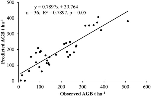
A simple linear regression analysis was used to cross-validate the predicted AGB data by using 36 plot AGB data. There was a strong relationship between plot AGB and predicted AGB as the relationship gave a strong coefficient of determination (R² = 0.79). Hence, the relationship exhibits that 79% of accuracy can be explained between observed plot AGB and predicted AGB (Figure 3). The AGB density map was predicted from the stepwise linear regression model between AGB plot-based and SAVI and ARVI. For predicting the total carbon stock of major land-use sectors, total AGB values were considered in the present study.

Figure 3. Scatter plot between predicted verses observed AGB.

Spatial distribution of carbon density and carbon sequestration

The estimated pooled data of AGB (trees, shrubs/saplings, herbs/seedlings) of major land-use sectors were used to prepare the spatial distribution map of the state. Total area coverage under each land-use was estimated from the classified LULC map of the state. It revealed that about 5,234,422 ha were covered by the dense forest, 1,590,022 ha under moderately dense forest, 316,688 ha under open forest. The total estimated vegetation carbon for the dense forest was 1416.69 MT (million tonnes), 327.12 MT for moderately dense forest and 42.98 MT for the open forest. Spatial carbon density map revealed an average carbon stock of 270.65 tones ha⁻¹, 205.75 tones ha⁻¹ and 135.72 tones ha⁻¹ in dense, moderately dense and open forests, respectively (Table 6) (Figure 4). The plantation forests in the state are very uncommon and their sizes vary greatly. Furthermore, most of the plantations are found in close vicinity of forest area and also in slopes of the hilly terrain. Plantation forest area is found to be very low as compared to the natural forests. Hence, keeping the above limitations into consideration, pixel-based classification of plantations was not feasible for the entire state so the total area covered by the plantations is not included in the land use map. However, the average carbon of plantations was calculated by delineating the sampled plantation sites and extrapolating the sampled plot values to the whole of the plantation sites. Carbon stock was recorded maximum in dense forest for both the years followed by plantation forests and the open forests. The rate of carbon accumulation in the Jhum lands was found to be largely regulated by the age of the lands. The differences in carbon stock change between the years 2016 and 2018 revealed that in all the land use, there is an increase in carbon stock from the first year to the third year. It was also observed that comparably higher carbon stock increase was recorded in Jhum field having age <5 years and >5 years which may be attributed to growth. Further, there were not many changes in soil carbon was observed between two sampling period in all the land-use systems. Carbon sequestration potential was more in <5 year Jhum fields (11.08 Mg C ha⁻¹yr⁻¹) followed by >5 year Jhum fields (8.15 Mg C ha⁻¹yr⁻¹), dense forests (7.39 Mg C ha⁻¹yr⁻¹), plantations (4.52 Mg C ha⁻¹yr⁻¹), moderately dense forest (0.90 Mg C ha⁻¹yr⁻¹), open forests (0.65 Mg C ha⁻¹yr⁻¹) and current Jhum fields (0.46 Mg C ha⁻¹yr⁻¹).

Figure 4. Spatial carbon density map of major landuse sectors in the State.

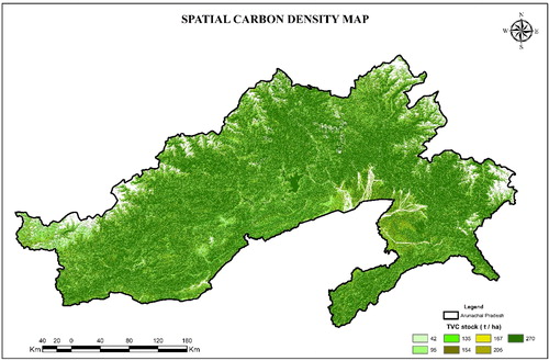
Table 6. Predicted total vegetation carbon of different land use sectors.

Land use sectors	AGB (A)	Mod_AGB (B)	AGBC (C = B*0.55)	BGBC (D = C*0.29)	HC (E)	SC (F)	TVC (G = C + D + E + F)
DF	332.28	358.64	197.25	57.20	2.30	13.90	270.65
MDF	246.63	268.48	147.67	42.82	2.14	13.12	205.75
OH	145.36	176.84	97.26	28.21	2.32	7.93	135.72
PL	179.31	196.20	107.91	31.29	2.26	12.72	154.18
JH > 5	149.63	228.18	125.50	36.39	1.72	4.00	167.61
JH < 5	55.40	129.11	71.01	20.59	1.17	2.26	95.03
CJH	16.84	54.50	29.97	8.69	1.24	2.11	42.01

Mod_AGB = Modeled AGB, HC = Herb carbon, SC = Shrub carbon, TVC = Total vegetation carbon, DF: Dense forest, MDF: Moderately dense forest, OF: Open forest, PL: Plantation, JH > 5: Jhum > 5 years, JH < 5: Jhum < 5 years, CJH: Current Jhum.

Future projection using CO₂FIX model

Spatial carbon simulation modeling for the whole study area was done using the CO₂FIX empirical model [46] which is a stand-level simulation model that quantifies the C stock in the forests and soil over time in a variety of ecosystems around the globe. It is a user-friendly tool for dynamically estimating the carbon sequestration potential. The model requires primary as well as secondary data on the land use types. In the present study, predicted AGBC (Above ground biomass carbon) data were considered instead of observed data to find out the differences in modeled predicted simulation for the year 2018 and observed data in the year of 2018.

Land-use change implication

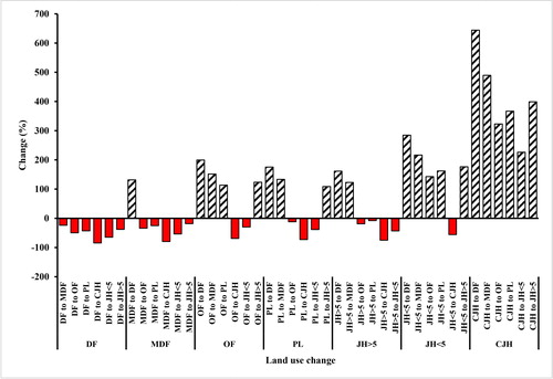
Land-use change significantly influences the rate of biomass accumulation thereby influencing the carbon cycle. Implications of the land-use change revealed that an amount of carbon will be emitted or sequestered based on the situation of major land-use sectors in the present study. Based on our experimental data transformation of the land uses to a balanced ecosystem can help in the accumulation of biomass. The maximum amount of carbon (84%) will be lost from dense forest once it is converted to current Jhum followed by Jhum <5 years (65%). There will be the lowest emission once such land use is converted to moderately dense forest. In the case of moderately dense forests, there will be a 132% increase in carbon sequestration when the moderately dense forest is converted to dense forest. However, if the open forests are either converted to moderately dense forests, plantation, or Jhum field >5 years there will be an increase in carbon sequestration rate at 123%, 176%,114% and 123%, respectively. If the plantation forests are converted to the dense forest or moderately dense forest it will sequester 176%, 133% of carbon however in other situations the carbon will be released by the plantation forest. If the current Jhum is being converted to other land use sector there will be carbon sequestration in the dense forests(644%), moderately dense forest (490%), open forest (323%), plantation (367%), Jhum <5 years (226%) and Jhum >5years (399%) respectively (Figure 5).

Figure 5. Future carbon stock simulation for selected landuse of the state using CO₂FIX model.

Discussion

The species richness of the present study may be compared with the findings of Kashung et al. [21] who recorded 164 tree species under 49 families from different land-use types of West Kameng district of Arunachal Himalaya. While Yam and Tripathi [48] reported 63 tree species from the Talle Wildlife Sanctuary of Arunachal Pradesh. Present density and basal area of woody species can be compared with the findings of Paul et al. [49] who recorded the density and basal area of Rhododendron tree species 16 stems/ha to 1422 stems/ha and 0.24 m²/ha to 131.30 m²/ha, respectively in the temperate broad-leaved forest of Arunachal Pradesh. Further, 477 stems/ha were reported from the Talle Wildlife Sanctuary of Arunachal Pradesh, which contributed to 43.06 m²/ha basal cover [48].

Likely the AGB reported from the present study can be compared with the AGB reported by various researchers working in the Eastern Himalayan region. Total AGB of different land-use sectors was reported to be maximum in the mixed dense forest (218.21 t/ha) followed by plantations (108 t/ha) and abandoned forest (84.94 t/ha) [21]. Further, Bordoloi et al. [50] reported AGB range of 102.04–316.18 t ha⁻¹ for different land-use sectors of Ziro valley, of Eastern Himalaya region.

The study stressed the optical satellite data-based VIs and their relationship with field-based plant biomass to predict the carbon stock, however, certain issues that influence the prediction capability of AGB and carbon are worth to be mentioned. The study region is located in highly undulating terrain with moderate to dense forest cover. Although the radiometric correction and terrain illumination effect correction approach was applied to minimize the influences that were caused due to haze and illumination. However, only small differences were observed in terms of reflectance properties and hence, can be attributed to uncertain slope and aspect in undulating terrain which might have influenced the VIs. These might have restricted the prediction capability of AGB and carbon stock. Further, sample plots were distributed on slightly to moderate inclined slopes having varied aspects. The sun and sensor geometry at the time of data acquisition also affects the complex reflectance properties of different earth surface features. The predictive model was derived from forest inventory and Landsat OLI based VIs. The study resulted that among the selected VIs, DVI performed less as compared to other vegetation indices. The DVI values observed in the present study showed a lower correlation to that of reported from Sindhudurg district of Maharashtra (R² = 0.76) of India [22, 51] using Landsat OLI sensor (R² = 0.58). The widely preferred index NDVI for AGB estimation and prediction was also used for comparing the results obtained with other indices. It resulted in a positive correlation with AGB (R² = 0.64) while had a very high saturation problem in the case of the area having high AGB stock. It was reported that the saturation could be mainly due to high reflectance in NIR as compared to low reflectance in the red band which could be responsible for poor correlation [39, 52]. Further, NDVI was more influenced by canopy, optical and geometrical orientation effect due to sun and sensor viewing angle [53].

The EVI showed a slightly better correlation which might be due to its capability to illuminate the atmospheric and canopy background effect. However, EVI also failed to address the more precise correlation as the slope and aspect variation in the study area is uncertain. It was reported that the terrain condition of the study region has a significant influence on EVI [54, 55]. Among all the indices, SAVI has superior performance as it uses the soil adjustment factor to minimize the soil brightness factor which influences the canopy reflectance properties and an improvement over NDVI in enhancing the vegetation mapping and AGB estimation [56, 57]. The SAVI performance (R² = 0.75) in AGB estimation can be compared with the result (R² = 0.85) reported by [51, 58]. The ARVI outperformed among all the VIs and showed (R² = 0.80) correlation with the AGB. The ARVI had an improvement in minimization of atmospheric aerosols brightness effect which influenced the surface reflectance properties [56, 59].

The stepwise multiple linear regression analysis was employed to predict the AGB estimation. The cross-validation of the model was also carried out by taking into consideration of 25% (36 plot) AGB data. It was observed from the model linear regression analysis of different vegetation indices that the SAVI (R² = 0.75, RMSE = 69.32 t ha⁻¹) and ARVI (R² = 0.80, RMSE = 61.52 t ha⁻¹) have a better correlation as these indices have shown higher R² value and low RMSE value which addressed best fit for model among all the VIs used in the study. The regression model in the present study incorporated SAVI and ARVI as predictor variables predicted a better AGB (R² = 0.85, RMSE = 53.21 t ha⁻¹) than that using individual Landsat OLI VIs. Hence, the findings of the present study demonstrate the use of Landsat OLI VIs as a predictor variable was successful in AGB prediction as these indices can maximize the sensitivity by minimizing the terrain, atmospheric and soil brightness effects [60]. The RMSE value obtained in the present study can be compared with the value reported using Landsat data [61–63].

The predicted AGB ranged from 54.5 to 358.64 t ha⁻¹ with an average of 201.7 t ha⁻¹ can be corroborated with the findings of other Landsat OLI based studies from the different region [51, 63–65]. Further, the estimated AGB was higher than the AGB (58 t ha⁻¹) reported from deciduous forests of India [66] and 72.54 t ha⁻¹ from the private forest of Indonesia [39]. However, it was lower than the AGB (230 t ha⁻¹) reported from the evergreen forest of Karnataka [24] and mangrove forest (250.53 t ha⁻¹) of Thailand [67]. Also, the estimated AGB (196.2 t ha⁻¹) in plantation forest can be compared with the AGB reported from Kodagu teak plantation (118.19 t ha⁻¹) [24] and 181.2 t ha⁻¹ in mangrove plantation of Odisha, India [68] while it was lower than AGB reported from plantation forest of Papum Pare district of Arunachal Pradesh [69] and plantation forest of southwestern Nigeria [70].

In order to access the Carbon stock and sequestration, the CO₂FIX model has been used in the present study, as the simplicity of the model which includes various modules that operate systemic manner and modules like products, bioenergy and finances are important for the futuristic simulation. The use of a cohort system in the CO₂FIX model made simple the process with more details in terms of different forest structures. Further, the model simulates and results in more complex stand dynamics with very minute details in each stand [71]. It was found that the predicted total vegetation carbon (TVC) in the year 2018 varied among the land-use sectors. Among the land-use sectors, the simulation model predicted lesser TVC for the year of 2018 in dense forest, Jhum >5 years and current Jhum compared to that observed TVC in 2018, however other land-use sectors have shown higher TVC compared to the observed TVC in 2018. Although the model is underestimating the carbon stock for different land use with modeled values of different years might be due to the limitations of component-based data input required during the modeling as well as sampling time (Figure 6).

Figure 6. Implications of landuse change on total carbon stock in different landuse sectors

Our study was confined to the sample locations where small or no change occurred in recent periods. As the study period is small but it is quite obvious that there was less sequestration of carbon stock from 2016 to 2018. However, if we analyze land use change implications in terms of anthropogenic activity or certain management activities like afforestation there will be gain or loss of sequestration based on the change in forest structure. The present study revealed that if the dense forest is once converted to other forest types there would be higher emission of carbon and loss in carbon stock. At the same time if the open forest, Jhum field were converted to improved forest type (moderate to dense crown cover) through various management activities there will be a noticeable amount of increase in carbon sequestration in the area. Hence, with the substantial increase in carbon sequestration in different land-use types, their conservation should be stimulated to mitigate the atmospheric CO₂ emissions [72, 73]. The restoration of the degraded forest is important to help in restricting the atmospheric CO₂ emissions and enhancing carbon sequestration [74, 75].

Conclusion

The findings of the present study showed that the maximum stand density was in Jhum land >5 years, followed by open forest, dense forest, moderately dense forest, plantations, Jhum <5 years and current Jhum fields. The maximum basal area was recorded in forests and plantations than the Jhum fields despite low stand density mainly due to the presence of a large number of individuals having more girth. The species richness is as follows: dense forests < open forests < moderate dense forests < plantations < Jhum fields. Maximum biomass was contributed by individuals having higher or intermediate girth class despite fewer individuals. The Landsat OLI derived vegetation indices are very much supportive in predicting AGB although there was some error in terms of surface reflectance problem due to terrain and sun and sensor position. However, applying various preprocessing operations enhances the reflectance properties of the earth's surface area which is evident in our study. Apart from this, there was no single VI that has promising results in predicting the AGB of sample plots, hence the combination of various VIs was included in the study for better prediction of AGB. In addition to this, other approaches like textural indices and machine learning, cellular automata, the artificial neural network can also be helpful in better prediction of AGB once applied successfully. The study also analyzed the land use implication to different forest types and showed that there will be more than double carbon sequestration, once the forest stands or Jhum land are restored. The conservation in different forest types would replenish the degraded ecosystem thereby increasing carbon sequestration. The present study will help the policymakers in visualizing a proper developmental goal, make some better decisions for the land-use change and achieving a higher carbon stock and maintaining balance in the global climate scenario.

Disclosure statement

No potential conflict of interest was reported by the author(s).

Correction Statement

This article has been republished with minor changes. These changes do not impact the academic content of the article.

References

- Pearson TRH,Brown S, Murray L, et al. Greenhouse gas emissions from tropical forest degradation: An underestimated source. Carbon Balance Manage. 2017;12(1):3.
- Qiu L, Zhu J, Wang K, et al. Land use changes induced county-scale carbon consequences in southeast China 1979–2020, evidence from Fuyang, Zhejiang province. Sustainability. 2015;8(1):38. doi:10.3390/su8010038.
- Pellikka PKE, Heikinheimo V, Hietanen J, et al. Impact of land cover change on aboveground carbon stocks in Afromontane landscape in Kenya. Appl Geogr. 2018;94:178–189. doi:10.1016/j.apgeog.2018.03.017.
- Houghton RA, House JI, Pongratz J, et al. Carbon emissions from land use and land-cover change. Biogeosciences. 2012;9(12):5125–5142. doi:10.5194/bg-9-5125-2012.
- Freibauer A, Rounsevell MDA, Smith P, et al. Carbon sequestration in the agricultural soils of Europe. Geoderma. 2004;122(1):1–23. doi:10.1016/j.geoderma.2004.01.021.
- IPCC. Mitigation of Climate Change. Contribution of Working Group III to the Fifth Assessment Report of the Intergovernmental Panel on Climate Change. Cambridge, UK and New York: Cambridge University Press; 2014.
- Pan Y, Birdsey RA, Fang J, et al. A large and persistent carbon sink in the world's forests. Science. 2011;333(6045):988–993. doi:10.1126/science.1201609.
- Gren IM, Aklilu AZ. Policy design for forest carbon sequestration: a review of the literature. For Policy Econ. 2016;70:128–136. doi:10.1016/j.forpol.2016.06.008.
- Yen TM. Comparing aboveground structure and aboveground carbon storage of an age series of moso bamboo forests subjected to different management strategies. J For Res. 2015;20(1):1–8. doi:10.1007/s10310-014-0455-0.
- Luo S, Wang C, Xi X, et al. Fusion of airborne LiDAR data and hyperspectral imagery for aboveground and belowground forest biomass estimation. Ecol Indic. 2017;73:378–387. doi:10.1016/j.ecolind.2016.10.001.
- UNFCCC. Reducing emissions from deforestation in developing countries: approaches to stimulate action. FCCC/SBSTA/2009/19/Add.1; 2009.
- Basuki TM, Van Laake PE, Skidmore AK, et al. Allometric equations for estimating the above-ground biomass in tropical lowland Dipterocarp forests. For Ecol Manag. 2009;257(8):1684–1694. doi:10.1016/j.foreco.2009.01.027.
- Qureshi A, Badola R, Hussain SA. A review of protocols used for assessment of carbon stock in forested landscapes. Environ Sci Policy. 2012;16:81–89. doi:10.1016/j.envsci.2011.11.001.
- DeFries R. Terrestrial vegetation in the coupled human-earth system: contributions of remote sensing. Annu Rev Environ Resour. 2008;33(1):369–390. doi:10.1146/annurev.environ.33.020107.113339.
- Dong J, Kaufmann RK, Myneni RB, et al. Remote sensing estimates of boreal and temperate forest woody biomass: carbon pools, sources, and sinks. Remote Sens Environ. 2003;84(3):393–410. doi:10.1016/S0034-4257(02)00130-X.
- Baccini A, Friedl MA, Woodcock CE, et al. Forest biomass estimation over regional scales using multisource data. Geophys Res Lett. 2004;31(10):1–4.
- Thenkabail PS, Enclona EA, Ashton MS, et al. Hyperion, IKONOS, ALI, and ETM + sensors in the study of African rainforests. Remote Sens Environ. 2004;90(1):23–43. doi:10.1016/j.rse.2003.11.018.
- Eckert S. Improved forest biomass and carbon estimations using texture measures from worldView-2 satellite data. Remote Sens. 2012;4(4):810–829. doi:10.3390/rs4040810.
- Deb D, Singh JP, Deb S, et al. An alternative approach for estimating above ground biomass using Resourcesat-2 satellite data and artificial neural network in Bundelkhand region of India. Environ Monit Assess. 2017;189(11):576.
- Das B, Deka S, Bordoloi R, et al. Rapid assessment of above ground biomass in forest of Papum Pare district of Arunachal Pradesh: a geospatial approach. Malaya J Bioresour. 2017;4(2):48–55.
- Kashung Y, Das B, Deka S, et al. Geospatial technology based diversity and above ground biomass assessment of woody species of West Kameng district of Arunachal Pradesh. For Sci Technol. 2018;14(2):84–90. doi:10.1080/21580103.2018.1452797.
- Das S, Singh TP. Correlation analysis between biomass and spectral vegetation indices of forest ecosystem. Int J Eng Res Technol. 2012;1(5):1–13.
- Foody GM, Boyd DS, Cutler MEJ. Predictive relations of tropical forest biomass from Landsat TM data and their transferability between regions. Remote Sens Environ. 2003;85(4):463–474. doi:10.1016/S0034-4257(03)00039-7.
- Devagiri GM, Money S, Singh S, et al. Assessment of above ground biomass and carbon pool in different vegetation types of south western part of Karnataka, India using spectral modeling. Trop Ecol. 2013;54(2):149–165.
- Gunawardena AR, Nissanka SP, Dayawansa NDK, et al. Estimation of above ground biomass in Horton Plains National Park, Sri Lanka using optical, thermal and RADAR remote sensing data. Trop Agric Res. 2015;26(4):608–623. doi:10.4038/tar.v26i4.8123.
- Gizachew B, Solberg S, Naesset E, et al. Mapping and estimating the total living biomass and carbon in low-biomass woodlands using Landsat 8 CDR data. Carbon Balance Manag. 2016;11(1):13.
- Civco DL. Topographic normalization of Landsat Thematic Mapper digital imagery. Photogramm Eng Remote Sens. 1989;55(9):1303–1309.
- Ricter R, Schlafer D. Atmospheric/Topographic correction for Satellite Imagery (ATCORE-2/3 Userguide Version 9.3.0, October 2019. Report DLR-IB 564-01/2019; 2019.
- Wu Q, Jin Y, Fan H. Evaluating and comparing performances of topographic correction methods based on multi-source DEMs and Landsat-8 OLI data. Int J Remote Sens. 2016;37(19):4712–4730. doi:10.1080/01431161.2016.1222101.
- Nath AJ, Tiwari BK, Sileshi GW, et al. Allometric models for estimation of forest biomass in North East India. Forests. 2019;10(2):103. doi:10.3390/f10020103.
- Richardson AJ, Wiegand CL. Distinguishing vegetation from soil background information. Photogramm Eng Remote Sens. 1977;43(12):1541–1552.
- Rouse JJW, Haas RH, Schell JA, et al. Monitoring vegetation systems in the Great Plains with ERTS. In: Freden SC, Mercanti EP, Becker MA, editors. Third Earth Resources Technology Satellite-1 Symposium. Technical presentations, Section A. Volume I. NASA SP-351. NASA, Washington, DC, USA; 1974. p. 309–317.
- Huete A. A soil-adjusted vegetation index (SAVI). Remote Sens Environ. 1988;25(3):295–309. doi:10.1016/0034-4257(88)90106-X.
- Kaufman YJ, Tanré D. Atmospherically Resistant Vegetation Index (ARVI) for EOS-MODIS. IEEE Trans Geosci Remote Sens. 1992;30(2):261–270. doi:10.1109/36.134076.
- Liu HQ, Huete A. A feedback based modification of the NDVI to minimize canopy background and atmospheric noise. IEEE Trans Geosci Remote Sens. 1995;33(2):457–465. doi:10.1109/TGRS.1995.8746027.
- Calvao T, Palmeirim JM. Mapping Mediterranean scrub with satellite imagery: biomass estimation and spectral behaviour. Int J Remote Sens. 2004;25(16):3113–3126. doi:10.1080/01431160310001654978.
- Ren H, Zhou G. Determination of green aboveground biomass in desert steppe using litter-soil-adjusted vegetation index. Eur J Remote Sens. 2014;47(1):611–625. doi:10.5721/EuJRS20144734.
- Sarker LR, Nichol JE. Improved forest biomass estimates using ALOS AVNIR-2 texture indices. Remote Sens Environ. 2011;115(4):968–977. doi:10.1016/j.rse.2010.11.010.
- Askar, Nuthammachot N, Phairuang W, et al. Estimating aboveground biomass on private forest using sentinel-2 imagery. J. Sens. 2018;2018:1–11. doi:10.1155/2018/6745629.
- Santos JR, Freitas CC, Araujo LS, et al. Airborne P-band SAR applied to the aboveground biomass studies in the Brazilian tropical rainforest. Remote Sens Environ. 2003;87(4):482–493. doi:10.1016/j.rse.2002.12.001.
- Urbazaev M, Thiel C, Migliavacca M, et al. Improved multi-sensor satellite-based aboveground biomass estimation by selecting temporally stable forest inventory plots using NDVI time series. Forests. 2016;7(12):169. doi:10.3390/f7080169.
- Nandy S, Singh R, Ghosh S, et al. Neural network-based modelling for forest biomass assessment. Carbon Manage. 2017;8(4): 305-317.
- Dong L, Du H, Han N, et al. Application of convolutional neural network on lei bamboo above-ground-biomass (AGB) estimation using Worldview-2. Remote Sens. 2020;12(6):958. doi:10.3390/rs12060958.
- Belsley DA. Conditioning diagnostics. Collinearity and weak data in regression. New York: Wiley; 1991.
- MacDicken KG. A guide to monitoring carbon storage in forestry and agroforestry projects. Winrock International Institute for Agricultural Development, Forest Carbon Monitoring Programme, Arlington, VA, USA; 1997.
- Schelhaas MJ, Van Esch PW, Groen TA, et al. CO2FIX V 3.1—A modelling framework for quantifying carbon sequestration in forest ecosystems. ALTERRA Report 1068. Wageningen, The Netherlands; 2004.
- Masera OR, Garza-Caligaris JF, Kanninen M, et al. Modeling carbon sequestration in afforestation, agroferstry and forest management projects: the CO2FIX V.2 approach. Ecol Model. 2003;164(2–3):177–199. doi:10.1016/S0304-3800(02)00419-2.
- Yam G, Tripathi OP. Tree diversity and community characteristics in Talle Wildlife Sanctuary, Arunachal Pradesh, Eastern Himalaya, India. J Asia Pac Biodivers. 2016;9(2):160–165. doi:10.1016/j.japb.2016.03.002.
- Paul A, Khan ML, Das AK. Population structure and regeneration status of rhododendrons in temperate mixed broad-leaved forests of western Arunachal Pradesh, India. Geol Ecol Landsc. 2019;3(3):168–186. doi:10.1080/24749508.2018.1525671.
- Bordoloi R, Das B, Yam G, et al. Carbon stock assessment of different land use sectors of Ziro Valley, Arunachal Pradesh using geospatial approach. J Geomat. 2019;13(2):262–270.
- Ali A, Ullah S, Bushra S, et al. Quantifying forest carbon stocks by integrating satellite images and forest inventory data. Aust J For Sci. 2018;135:93–117.
- Thenkabail PS, Smith RB, De Pauw E. Hyperspectral vegetation indices and their relationships with agricultural crop characteristics. Remote Sens Environ. 2000;71(2):158–182. doi:10.1016/S0034-4257(99)00067-X.
- Chen JM, Cihlar J. Retrieving leaf area index of boreal conifer forests using Landsat TM images. Remote Sens Environ. 1996;55(2):153–162. doi:10.1016/0034-4257(95)00195-6.
- Matsushita B, Yang W, Chen J, et al. Sensitivity of the Enhanced Vegetation Index (EVI) and Normalized Difference Vegetation Index (NDVI) to topographic effects: a case study in high-density cypress forest. Sensors. 2007;7(11):2636–2651. doi:10.3390/s7112636.
- Garroutte EL, Hansen AJ, Lawrence RL. Using NDVI and EVI to map spatiotemporal variation in the biomass and quality of forage for migratory elk in the greater Yellowstone ecosystem. Remote Sens. 2016;8(5):404. doi:10.3390/rs8050404.
- Huete AR, Liu HQ. An error and sensitivity analysis of the atmospheric- and soil-correcting variants of the NDVI for the MODIS-EOS. IEEE Trans Geosci Remote Sens. 1994;32(4):897–905. doi:10.1109/36.298018.
- Vidhya R, Vijayasekaran D, Farook MA, et al. Improved classification of mangroves health status using hyperspectral remote sensing data. Int Arch Photogramm Remote Sens Spatial Inf Sci. 2014;XL-8(8):667–670. doi:10.5194/isprsarchives-XL-8-667-2014.
- Kumar D, Shekhar S. Statistical analysis of land surface temperature-vegetation indexes relationship through thermal remote sensing. Ecotoxicol Environ Saf. 2015;121(2):39–44. doi:10.1016/j.ecoenv.2015.07.004.
- Tanré D, Deroo C, Duhaut P, et al. Technical note. Description of a computer code to simulate the satellite signal in the solar spectrum: the 5S code. Int J Remote Sens. 1990;11(4):659–668. doi:10.1080/01431169008955048.
- Günlü A, Ercanli İ, Ba EZ, et al. Estimating aboveground biomass using Landsat TM imagery: a case study of Anatolian Crimean pine forests in Turkey. Ann For Res. 2014;57(2):289–298.
- Powell SL, Cohen WB, Healey SP, et al. Quantification of live aboveground forest biomass dynamics with Landsat time-series and field inventory data: a comparison of empirical modeling approaches. Remote Sens Environ. 2010;114(5):1053–1068. doi:10.1016/j.rse.2009.12.018.
- Avitabile V, Baccini A, Friedl MA, et al. Capabilities and limitations of Landsat and land cover data for aboveground woody biomass estimation of Uganda. Remote Sens Environ. 2012;117:366–380. doi:10.1016/j.rse.2011.10.012.
- Li B, Wang W, Bai L, et al. Estimation of aboveground vegetation biomass based on Landsat-8 OLI satellite images in the Guanzhong Basin, China. Int J Remote Sens. 2019;40(10):3927–3947. doi:10.1080/01431161.2018.1553323.
- Suhardiman A, Tampubolon BA, Sumaryono M. Examining spectral properties of Landsat 8 OLI for predicting above-ground carbon of Labanan Forest. IOP Conf Ser: Earth Environ Sci. 2018;144:012064. doi:10.1088/1755-1315/144/1/012064.
- López-Serrano PM, Cárdenas Domínguez JL, Corral-Rivas JJ, et al. Modeling of aboveground biomass with Landsat 8 OLI and machine learning in temperate forests. Forests. 2019;11(1):11. doi:10.3390/f11010011.
- Thumaty KC, Fararoda R, Middinti S, et al. Estimation of above ground biomass for central Indian deciduous forests using ALOS PALSAR L-band data. J Indian Soc Remote Sens. 2016;44(1):31–39. doi:10.1007/s12524-015-0462-4.
- Jachowski NR, Quak MS, Friess DA, et al. Mangrove biomass estimation in Southwest Thailand using machine learning. Appl Geogr. 2013;45:311–321. doi:10.1016/j.apgeog.2013.09.024.
- Sahu SC, Kumar M, Ravindranath NH. Carbon stocks in natural and planted mangrove forests of Mahanadi Mangrove Wetland, East Coast of India. Curr Sci. 2016;110(12):2253–2260. doi:10.18520/cs/v110/i12/2253-2260.
- Bordoloi R, Das B, Tripathi OP. Biomass estimation in plantation forests of Papum Pare district of Arunachal Pradesh, India. Malaya J Biosci. 2017;4(2):63–70.
- Ola-Adams BA. Effects of spacing on biomass distribution and nutrient content of Tectonagrandis Linn. f. (teak) and Terminalia superba Engl. & Diels. (Afara) in south-western Nigeria. For Ecol Manage. 1993;58(3–4):299–319. doi:10.1016/0378-1127(93)90152-D.
- Kim H, Kim YH, Kim R, et al. Reviews of forest carbon dynamics models that use empirical yield curves: CBM-CFS2, CO2FIX, CASMOFOR, EFSCEN. For Sci Technol. 2015;11(4):212–222. doi:10.1080/21580103.2014.987325.
- FAO Global Forest resource Assessment 2005, FAO, Rome; 2006.
- Canadell JG, Raupach MR. Managing forests for climate change mitigation. Science. 2008;320(5882):1456–1457. doi:10.1126/science.1155458.
- Silver WL, Ostertag R, Lugo AE. The potential for carbon sequestration through reforestation of abandoned tropical agricultural and pasture lands. Restor Ecol. 2000;8(4):394–407. doi:10.1046/j.1526-100x.2000.80054.x.
- Grünzweig JM, Gelfand I, Fried Y, et al. Biogeochemical factors contributing to enhanced carbon storage following afforestation of a semi-arid shrubland. Biogeosciences. 2007;4(5):891–904. doi:10.5194/bg-4-891-2007.