The greenhouse gas benefits of corn ethanol – assessing recent evidence

Abstract

In 2010, the U.S. Environmental Protection Agency (EPA) released a life-cycle analysis of the greenhouse gas (GHG) emissions associated with the production and combustion of corn ethanol. EPA projected that by 2022, the emissions profile of corn ethanol from a new refinery would be 21% lower than that of an energy equivalent quantity of gasoline. Since 2010, the 21% value has dominated policy discussions and federal regulations related to corn ethanol as a renewable fuel and a GHG mitigation option. It is now 2018 and new data, scientific studies, technical reports, and other information allow us to examine the emissions pathway corn-ethanol has actually followed since 2010. Using this information, we assess corn ethanol's current GHG profile at 39–43% lower than gasoline. We also develop two projected emissions scenarios for corn ethanol in 2022. These scenarios highlight opportunities to produce ethanol with emissions that are 47.0–70.0% lower than gasoline. Many countries are now developing or revising renewable energy policies. Typically, biofuel substitutes for gasoline are required to reduce GHG emissions by more than 21%. Our results could help position U.S. corn ethanol to compete in these new and growing markets.

Keywords:

• Ethanol
• corn
• greenhouse gas
• life cycle analysis

Introduction

Between 2004 and 2014, US ethanol production, virtually all from cornstarch, increased from 12.87 to 54.13 billion liters per year. This increase was driven by two pieces of legislation that mandated the nation’s supply of transportation fuel, in aggregate, must contain specific amounts of biofuels. The Energy Policy Act of 2005 established the Renewable Fuel Standard (RFS), which included a schedule of required biofuel use that started at 15.14 billion liters in 2006 and rose to 28.39 billion liters by 2012. The Energy Independence and Security Act of 2007 replaced the RFS with the Revised Renewable Fuel Standard (RFS2). The RFS2 included a new schedule of required biofuel use that began at 34.07 billion liters in 2008 and ramps up to 136.26 billion liters by 2022. Corn ethanol’s mandate started at 34.07 billion liters in 2008, increased to 56.78 billion liters in 2015, and remains at that level through 2022.

A key objective of the RFS2 is to reduce greenhouse gas (GHG) emissions associated with transportation fuels. Currently, the only cost-effective biofuel substitute for gasoline is ethanol. Under the RFS2, ethanol can qualify as a conventional, advanced, or cellulosic biofuel. Conventional biofuel is defined as ethanol made from cornstarch. To be a renewable fuel, corn ethanol produced in refineries that began construction on or after 19 December 2007 must have life-cycle GHG emissions at least 20% lower than an energy-equivalent quantity of average gasoline in 2005.¹ Corn ethanol produced in refineries in place or under construction on that date is grandfathered in as conventional biofuel regardless of its GHG profile. Ethanol made from cellulose, hemi-cellulose, lignin, sugar, starch (not from corn), and various types of waste biomass that has life-cycle GHG emissions at least 50% lower than those of gasoline qualify as ‘advanced biofuels’. Additionally, ethanol made from cellulose, hemi-cellulose, or lignin that has a GHG profile at least 60% lower than that of gasoline qualifies as ‘cellulosic biofuel’. Over time, advanced and cellulosic biofuels receive increasing shares of the annual renewable fuel mandate.

Quantifying the GHG profile of corn ethanol has been contentious since Searchinger et al. [2] concluded that the emissions associated with its production and combustion exceeded the emissions associated with producing and combusting an energy-equivalent quantity of gasoline. The authors argued that using billions of kilograms of US corn to produce ethanol reduces supplies of, and increases prices for, corn and other commodities in domestic and world food and feed markets. Farmers in the United States and elsewhere respond by bringing new land into production. These land-use changes (LUC) are related to ethanol production because the new land is used to grow more corn and to replace some of the decreased production of other commodities that occurs when US farmers allocate more existing cropland to corn. Searchinger et al. [2] argued that including emissions related to LUC, particularly international LUC (iLUC), results in corn ethanol having a higher GHG profile than gasoline.

The RFS2 directed the US Environmental Protection Agency (EPA) to do a full GHG life-cycle analysis (LCA) for corn ethanol and to include both direct and significant indirect sources of emissions. EPA designated iLUC, international livestock, international rice methane, and international farm inputs as significant indirect sources. The LCA was released in the 2010 Regulatory Impact Analysis (RIA) of the RFS2 [1]. It included projections through 2022 of the GHG emissions associated with 11 source categories that, collectively, capture the full range of direct and indirect GHG emissions associated with the production and combustion of corn ethanol. The EPA concluded that in 2022, the emissions profile of a unit of corn ethanol from a new natural gas-powered refinery would be 21% lower than the emissions profile of an energy-equivalent quantity of ‘average’ gasoline in 2005.

Since 2010, the RIA LCA for corn ethanol has dominated policy discussions and federal regulations related to ethanol as a renewable fuel and a GHG mitigation option. During this time, a large body of new data, scientific studies, technical reports, and other information has become available collectively showing that the emissions pathway corn ethanol has followed since 2010 is much lower than that projected in the RIA. Our objective is to assess corn ethanol’s current GHG profile in light of this new information. This work is timely as many countries (e.g. Colombia, Japan, Brazil, Canada and the European Union) are developing renewable energy policies that require biofuel substitutes for gasoline to reduce GHG emissions by more than 21%. Our results could help position US corn ethanol to compete in these new and growing markets.

We also develop two projected emissions profiles for corn ethanol in 2022. A business-as-usual (BAU) scenario assumes a continuation through 2022 of several trends that have been reducing corn ethanol’s GHG profile over time (e.g. refineries switching from coal to natural gas as a process fuel). A high efficiency-high conservation (HEHC) scenario assumes a proactive approach by refineries to lower the GHG profile of ethanol. In addition to the BAU trends, this scenario assumes refineries adopt specific GHG emissions-reducing technologies and practices. The results of this scenario could apply to a refinery, a set of refineries, or the industry as a whole.

Methods

In 2010, the RIA LCA was the most comprehensive assessment of corn ethanol’s GHG profile. EPA developed three scenarios to assess the impacts of the RFS2’s ethanol mandate. A ‘reference case’ considered the situation with no RFS2. Projected volumes in 2022 of corn ethanol, soybean biodiesel, and cellulosic ethanol (46.56, 0.38, and 0.0 billion liters, respectively) were taken from the Energy Information Agency's (EIA) Annual Energy Outlook for 2007 [3]. A ‘control case’ included the renewable fuel volumes mandated by the RFS2 by 2022. For corn ethanol, soybean biodiesel, and cellulosic ethanol these are, respectively, 56.78, 2.27, and 48.45 billion liters. A ‘corn ethanol only case’ set corn ethanol at its reference case volume and soybean diesel and cellulosic ethanol at their 2022 RFS2 levels. Comparing the control and corn ethanol only cases isolated the impacts of the corn ethanol mandate.

The RIA LCA is the starting point for our analysis. For each of the 11 emissions categories we: (1) review the RIA projection; (2) describe relevant new information that has become available since 2010; and (3) quantify a new emissions value based on the new information.² For some categories, no substantive new information has appeared since 2010. In these cases, we apply, as appropriate, new emissions coefficients and global warming potentials (GWPs) to the RIA values. For source categories where new information indicates that emissions have not developed as projected in the RIA, we use a variety of methods to derive new emissions values. In some cases, our methods differ from those used in the RIA. This is particularly true for categories where emissions reflect changes in domestic and international land use.

Most of the new data, emission factors (EFs), and global warming potentials we use in this analysis have become available from 2010 to 2015. Most of the studies we draw on have publication dates between 2013 and 2015. This means our current GHG profile does not reflect a specific year but rather a composite year representative of the mid-2010s. Finally, in developing updated emissions values we use a variety of metrics. To aggregate emissions across categories and facilitate comparisons with RIA emissions values, we convert the total emissions for each category to the RIA metric, grams of CO₂ equivalent per million Btu (g CO₂e/MMBtu).³

Results

Domestic farm inputs and fertilizer N₂O

This category includes emissions related to the on-farm use of fertilizers, other chemicals, fossil fuels, and purchased electricity. We also include here an emissions credit that accounts for emissions reductions associated with substituting ethanol co-products for grains in livestock diets.

EPA used the Forestry and Agricultural Sector Optimization Model (FASOM) to assess the US farm sector impacts of the RFS2 on production, land use, and input use. FASOM is a dynamic partial equilibrium economic model that disaggregates US agriculture into 11 market regions and 63 sub-regions [4]. The model includes over 2000 crop, livestock, and biofuel production systems. In FASOM simulations, lands shift between commodities in response to new policy or market conditions and the model tracks changes, by commodity, in acres, production and input use (including nitrogen, phosphorus, potash, herbicides, pesticides, diesel, gasoline, natural gas, and electricity). Life-cycle EFs for fuels and fertilizers are from Argonne National Laboratory (ANL)’s GREET 2009 model. EFs for fertilizer-related N₂O are from Colorado State University’s DAYCENT model. Comparing simulation results for the ‘control’ and ‘corn only’ cases, the RIA emissions value for this category was 10,313 g CO₂e/MMBtu [1].

The RIA projected 19.66 million additional tonnes of corn would be needed by 2015 to produce the 9.84 billion liters of ethanol required to meet the RFS2’s 56.78 billion liter cap. Since the overall mandate was 55.98 billion liters in 2014 and 56.78 billion liters thereafter, we use the RIA corn projection as the basis for assessing the current emissions for this source category. Dividing 19.66 by the average US per-hectare corn yield in 2015 of 10.57 tonnes, we estimate the RFS2 corn ethanol mandate would require US farms to increase corn area by 1.86 million hectares.⁴ We allocate these acres regionally based on corn acreage data in the United States Department of Agriculture's (USDA) 2010 Agricultural Resource Management Survey (ARMS) [6].

For inputs, we consider changes in farm sector use of nitrogen (N), phosphorus (P), and potassium (K); composites for herbicides, insecticides, and fungicides; and diesel fuel. We get chemical application rates for corn, nationally and by region, from the 2010 ARMS [6].⁵ For fungicide, ARMS data identify application rates for the Corn Belt and the nation. For non-Corn Belt regions, we use the national rate. Based on University of Tennessee farm budgets for 2015 [7], we set diesel fuel use at 72.36 L/ha under conventional tillage. To account for hectares on which a given chemical is not applied, we calculate an effective application rate by multiplying the ARMS regional application rate by the percentage of hectares in each region that apply that chemical [6].⁶ Our region-weighted national average effective application rates for nitrogen, phosphorus, potassium, herbicides insecticides, and fungicides are 155.27, 53.55, 54.34, 2.36, 0.02, and 0.01 kg/ha, respectively. Regional effective application rates are available in Rosenfeld et al. [5].

From the regional acreage changes and effective application rates, we obtain changes in chemical and fuel use by US agriculture in response to the RFS2 corn ethanol mandate. Multiplying these changes by EFs from several sources, we get corresponding emissions estimates. Energy-related emissions also occur in the manufacture and transport of chemicals and fuel inputs. EFs reflecting these ‘upstream’ activities for nitrogen, phosphorus, potassium, and insecticides are obtained from the GREET 2015 model [8]. From GREET 2015 we also obtain EFs for diesel fuel covering both upstream activities and on-site combustion. EFs covering upstream activities for herbicides and fungicides come from the ecoinvent v2 database [9]. For nitrogen fertilizer applications, N₂O is emitted directly to the atmosphere from cultivated soils, and indirectly at other locations when N is transported off-site through volatilization, leaching, and runoff. EFs for these direct and indirect N₂O emissions follow IPCC guidance per kilogram of N fertilizer applied [10].

We assess emissions related to fertilizers, herbicides and pesticides and fuel at 10,815, 8382, and 2617 g CO₂e/MMBtu, respectively. Summing these values, we estimate the total emissions-related domestic use of farm chemicals and fuel at 21,814 g CO₂e/MMBtu. Our approach differs from the RIA’s, which simultaneously accounts for the substitution of ethanol co-products for grain in animal feed markets, resulting in a reduction in additional corn production (and therefore hectares) required to meet the RFS2 ethanol mandate. Our use of regional effective application rates means our emissions estimates apply to ‘representative’ incremental regional acres.⁷ Hence, we still need to account for the co-product emissions credit.

Animal feed co-products from ethanol production include distiller grains and solubles (DGS) from dry milling and corn gluten meal and corn gluten feed (CGM and CGF) from wet milling. We use the ‘displacement method’ to assess the co-product credit. In this approach, all energy and emissions associated with separating solids from the ethanol stream, drying the solids, and transporting the finished feeds to the point of final sale are allocated to the ethanol pathway. The pathway then receives a credit equal to the emissions that would have occurred if the displaced feed grain had been produced. GREET 2015 includes values for displaced animal feed per unit of ethanol by milling process. Table 1 shows these values and the co-product emissions credits per liter of ethanol and per MMBtu.

Table 1. Ethanol production market breakdown and animal feed displacement by ethanol plant type.

Ethanol plant type	Ethanol market share (%)	Total displaced animal feed (g/L of ethanol)				Co-product credit
		Corn	Soybean meal	Urea	Soy oil	g CO2e/L ethanol	g CO2e/MMBtu
Dry mill w/o corn oil extraction	17.7	527	207	15.3	–	−262	−12,981
Dry mill w/corn oil extraction	70.9	504	198	14.6	–	−250	−12,417
Wet mill	11.4	857	–	13.1	117	−291	−14,449
Weighted average		–	–	–	–	−257	−12,749

Summing the farm inputs emissions (+21,814 g CO₂e/MMBtu) and the weighted average co-product credit (−12,749 g CO₂e/MMBtu) gives a total emissions value of 9065 g CO₂e/MMBtu. This is slightly lower than the RIA value and largely reflects the lower GWP for N₂O from the Intergovernmental Panel on Climate Change's (IPCC) Fourth Assessment Report (AR4). EPA used GWPs from the IPCC's Second Assessment Report (AR2).

Domestic land-use change

Domestic LUC includes: (1) direct land-related emissions associated with shifting cropland and land from other uses into corn production; and (2) indirect emissions related to bringing new lands into production to replace some of the decreases in output of non-corn commodities that occur when farmers allocate more existing cropland to corn. For the RIA, EPA used FASOM to estimate domestic LUC and the associated emissions. FASOM tracks carbon stored in trees, understory, and litter within forests and plantations of woody energy crops but excludes carbon stored in cultivated crops. For agricultural lands, FASOM CO₂ and N₂O EFs are from the DAYCENT/CENTURY model.

EPA compared FASOM LUC results from the control and corn only scenarios. For each scenario, the model summed LUC emissions over the period 2000–2022. To these values were added cumulative land-related emissions that occur in the 30 years following 2022 (reflecting continuing emissions from agricultural soils, decaying biomass, and wood products). For total cropland and total corn area the net changes were 0.581 and 1.477 million hectares, respectively. The difference in annualized emissions between the two scenarios was −4000 g CO2e/MMBtu, which was the RIA emissions value for this category [1].

We estimate domestic LUC emissions using results of a 2013 simulation of the Global Trade Analysis Project-Biofuels (GTAP-Bio) model and LUC emissions coefficients available in ANL’s Carbon Calculator for Land Use Change from Biofuels Production (CCLUB) tool [11]. The GTAP-Bio 2013 results, developed in Taheripour and Tyner [12], include domestic and international land-use changes related to US corn ethanol production increasing from its 2004 level (GTAP-Bio’s base period) to the RFS2 cap of 56.78 billion liters per year. Globally, the GTAP-Bio model estimates regional area changes for 18 agro-ecological zones (AEZs), and within each AEZ, changes in four land types (forests, grassland, cropland-pasture, and young forest shrub). Only AEZs 7–16 apply to US agriculture. For the United States, summing area changes across AEZs shows increasing US ethanol production resulted in conversions to cropland of 13,999 hectares of young forest shrub, 64,773 hectares of forest, 92,617 hectares of grassland and 1,788,462 hectares of cropland pasture (conversions by AEZ and land type are in Rosenfeld et al. [5, table 2-12]).

Table 2. Domestic land-use change emissions for GTAP 2013 simulation using emission factors from Century/COLE, Woods Hole, and Winrock International.

	Total direct emissions (Mg CO2e)	Annualized emissions (Mg CO2e/year)	Direct emissions (g CO2e/L)	Direct emissions (g CO2e/MMBtu)
Century/COLE – 30 cm – Reduced till	−52,191,279	−1,739,709	−39.65	−1965
Century/COLE – 100 cm – Reduced till	−62,656,429	−2,088,548	−47.60	−2359
Century/COLE – 30 cm – Conventional till	−45,625,214	−1,520,840.5	−34.66	−1718
Century/COLE – 100 cm – Conventional till	−54,120,694	−1,804,023.1	−41.13	−2038
Woods Hole	48,163,909	1,605,464	36.59	1813
Winrock International	280,879,558	9,362,652	213.4	10,577

Table 3. Methane emission factors from irrigated rice by region (in kg CO₂e/ha).

Study	Corn belt	Pacific Southwest	South central	Southeast	Southwest	United States
EPA RIA^a	4512	4406	5557	N/A	10,811	N/A
Present^b	5928	5310	7500	9222	11,421	7324

Sources: ^a [1, Table 2.4-9]; ^b [21]; N/A = not applicable; kg CO₂e/ha = kilograms of carbon dioxide equivalent per hectare.

Table 4. Changes in population, emission factors, and total emissions by livestock type.

Livestock type	Change in population (in 1000 head)	Enteric emissions		Manure management emissions		Total g CO2e/MMBtu
		per head (g CO2e/head)	Total emissions (g CO2e/MMBtu)	per head (g CO2e/head)	Total emissions (g CO2e/MMBtu)
Dairy	−20^a	3625	−351	2065	−200	−551
Beef	90	1850	807	143	62	869
Poultry	−12,564.6^b	–	NA	3.21	−195	−195
Swine	−220	37.5	−40	378	−403	−443
Total	NA	NA	416	NA	−736	−320

^a Mature cows only.

^b Population changes the same as in [1] except for poultry, which has been reduced to reflect annual average population changes rather than changes in total head slaughtered.

g CO₂e/head = grams of carbon dioxide equivalent per head; g CO₂e/MMBtu = grams of carbon dioxide equivalent per million British thermal units.

Table 5. Reduced Methane Emissions from Distillers Grains as Animal Feed by Ethanol Plant Type.

Ethanol plant type	Ethanol market share (%)	Dried DGS yield (g/L)	Wet DGS yield (g/L)	Emissions reduced (g CO2e/L)	Emissions reduced (g CO2e/MMBtu)
Dry mill with out corn oil extraction	17.7	504.1	661.7	−50.46	−2506
Dry mill with corn oil extraction	70.9	482.2	632.9	−48.34	−2397
Wet mill	11.4	–	–	–	–
Per average liter	–	431.1	565.9	−43.21	−2143

g/L: grams per liter; g CO₂e/L: grams carbon dioxide equivalent per liter; g CO₂e/MMBtu: grams carbon dioxide equivalent per million British thermal units.

Table 6. iLUC emissions by scenario, emissions factor set, and annualized emissions value.^a

Scenario	Emission factor (EF) data set	Emissions (g CO2e/MMBtu)^c
	RIA [1] analysis
FAPRI-CARD	Winrock	31,790
	Scenarios making up composite iLUC emissions value used in this analysis
GTAP 2013	CARB AEZ Model	17,802
GTAP 2013^b	Winrock	5913
GTAP 2013 adjusted with data in [26]	CARB AEZ Model	8464
GTAP 2013 adjusted with data in [26]	Winrock	1326
CARB 2015 [27]	CARB AEZ Model	20,890
Dunn et al. 2015 [11]	Winrock	5286
[11]	Woods Hole	3893

^a Scenarios in [11] and the four scenarios we construct use land conversion results published by [26]. [27] modified some important factors and values within the GTAP-Bio model to produce their own unique land conversion results.

^b Emissions vary in these studies because within each region, [11] used an average of the individual country EFs, while we weight countries’ EFs by their share of regional arable land.

^c All studies assume emissions from land conversions occur over 30 years. This column shows annualized values. The RIA and GTAP-Bio 2013 consider different volume increases in corn ethanol production. Describing emissions in g CO₂e/MMBtu puts all emissions in a comparable metric.

Abbreviations: iLUC = international Land Use Change; g CO₂e/MMBtu = grams carbon dioxide eqivalent per million British thermal units; RIA = Regulatory Impact Analysis; FAPRI- CARD = Food and Agricultue Policy Research Institute-Center for Agricultural and Rural Research model; GTAP = Global Trade Analysis model; CARB = California Air Resources Board; AEZ = Agricultural-Ecological Zone.

Table 7. Mode and distance assumptions.

Mode	Farm to stacks		Stacks to plant		Plant to blending terminal		Terminal to retail station		DGS^a		Corn oil
	% of total shipped	Distance (km)	% of total shipped	Distance (km)	% of total shipped	Distance (km)	% of total shipped	Distance (km)	% of total shipped	Distance (km)	% of total shipped	Distance (km)
Barge	0	0.0	0	0.0	13	837	0	0.0	2	837	0	0
Rail	0	0.0	0	0.0	79	1287	0	0.0	12	1287	20	644
Truck	100	16.1	100	64.4	8	129	100	48.3	86	80	80	161

^a The values shown in these columns reflect a weighted average dry and wet distiller grains and solubles (DGS) co-product.

Table 8. Assumptions and inputs for fuel production modeling in GREET 2015.

Input category	Dry milling plant without corn oil extraction^a	Dry milling plant with corn oil extraction^a	Wet milling plant^b
Total energy use for ethanol production (MJ/L)	28.33	27.88	50.02
Process fuel energy – natural gas, coal, and biomass (MJ/L)	25.66	25.18	50.02
Electricity use (kWh/L)	0.195	0.198	0.00
Co-product yield – dry DGS to animal feed (g/L ethanol)	504	482	0.00
Co-product yield – wet DGS to animal feed (g/L ethanol)	661	633	0.00
Co-product yield – CGM to animal feed (g/L ethanol)	0.00	0.00	162
Co-product yield – CGF to animal feed (g/L ethanolc	0.00	0.00	702
Co-product yield: Corn oil (actual g/L ethanol)	0.00	22.77	117
Ethanol yield (L/bushel)	10.6	10.7	9.88
GHG emissions (g CO2e/MMBtu)	32,114	31,590	53,055

^a These are composite refineries reflecting the 2014 mix of natural gas, coal, and biomass as a process fuel at the respective dry mill refineries.

^b Electricity consumption is included with process fuel energy.

Abbreviations: GREET = The Greenhouse Gas, Regulated Emissions, and Energy Use in Transportation Model; MJ/L =Mega Joules per liter;

kWh/L = kilowatt hours per liter; g/L = grams per liter; L/bushel = liters per bushel; g CO₂e/MMBtu = grams CO2 equivalent per million Britsh thermal unit; RIA = Regulatory Impact Analysis; BAU = Business as Usual Scenario; HEHC = High Efficiency - High Conservation Scenario

The CCLUB tool also includes LUC results for a similar analysis by Taheripour, Tyner, and Wang using a 2011 GTAP model [13]. Comparing the 2011 and 2013 GTAP results highlights how much new information has improved our understanding of the links between, and impacts related to, changes in corn ethanol markets and LUC relative to 2010. GTAP-Bio expands the set of land transformation elasticities from a single value to a set of region-specific values. GTAP-Bio also incorporates an improved cost structure that reflects the higher cost of converting forest to cropland versus converting pasture to cropland. Comparing the LUC results, conversions of young forest shrub, forest, and grasslands in the 2013 GTAP-Bio simulation are 79%, 80%, and 86% less, respectively, than in the 2011 simulation. There is also a 53% increase in conversions of cropland pasture to cropland. Overall, the GTAP-Bio analysis shows the large increase in US corn ethanol production since 2004 resulted in a large increase in land in corn production, a relatively small increase in aggregate agricultural land, and increases in cropland coming predominantly (over 90%) from cropland pasture.

We pair the GTAP-Bio AEZ-land type area changes with LUC emissions coefficients from the Century/COLE model. Relative to the RIA, which uses 2010 Century coefficients for agricultural land emissions, the coefficients used in our analysis better reflect irrigation effects and N₂O emissions from cropland and pasture.

The CCLUB tool also includes LUC emissions coefficients from Woods Hole (WH), and Winrock International (WI). We chose the Century/COLE coefficients because they align with the GTAP-Bio’s AEZ-land-use type structure. The WH and WI coefficients apply to regions and have fewer land types. The WH coefficient set includes forest and grasslands; the WI set includes forest, grassland, and cropland-pasture. Hence, using the WH or WI coefficients with the AEZ-land type requires some aggregation across AEZs and land types. Additionally, distinct Century/COLE EFs are available for conventional and reduced tillage systems and soil depths of 30 and 100 cm. We assume the 100 cm soil-depth coefficients present a more complete picture of soil carbon changes than the 30 cm coefficients. We also note the conventional tillage scenarios are slightly less in absolute value (i.e. more conservative) than the reduced tillage coefficients. Based on these considerations, we use Century/COLE 100 cm conventional tillage coefficients to estimate the GHG emissions related to agricultural lands. The Century/COLE EFs by AEZ and land type for conventional and reduced tillage systems and soil depths of 30 cm and 100 cm are in Rosenfeld et al. [5, tables 2-14 and 2-15].

We aggregate emissions across all AEZ-land type combinations and then annualize the total using the CCLUB default value of 30 years. We divide these emissions by 43.87 (i.e. the increase in annual ethanol production, in billion liters, from 2004 to the RFS2 cap of 56.78 billion liters) to get emissions per billion liters of increased annual ethanol production. We convert these emissions to the common metric g CO₂e/MMBtu using a heating value of 20,166 Btu/L.

As shown in Table 2, our emissions value for the domestic LUC category is −2038 g CO₂e/MMBtu. The negative value indicates net sequestration associated with all ethanol-related LUC. This sequestration is due to: (1) over 90% of all new lands shifting into cropland coming from the cropland pasture category; and (2) the Century/COLE emissions coefficients for such conversions being negative across all AEZs. The net sequestration associated with conversion of cropland pasture to cropland reflects root growth deeper in the soil profile that more than offsets CO₂ emissions due to oxidation of carbon near the surface. Net emissions associated with conversions of forest, grassland, and young forest shrub are all positive. For completeness, Table 2 also shows domestic LUC emissions for our land use changes using the WH and WI EFs and the Century/COLE emissions factor for reduced tillage and 30 cm soil depth.

Finally, several recent studies examine changes in US agricultural land use between 2006 and 2012 using USDA's Cropland Data Layer (CDL) series. These studies conclude that over this period, increases in US corn ethanol production helped shift millions of acres from grassland uses (and some forest and wetland uses) to cropland, and produced a large increase in cropland acres planted to corn and corn/soybean systems. Wright and Wimberly [14], Lark et al. [15], and Wright et al. [16] extend the grassland conversion results to significant losses of native prairie and other long-term grasslands, and to previously unaccounted-for GHG emissions attributable to corn ethanol. Lark et al. [15] put the GHG emissions from recently converted lands used to grow corn or soybeans at 94–186 MMTCO₂e. For reasons developed below, we do not incorporate the results of these studies in our analysis.

The CDL is a land cover data product developed annually by USDA's National Agricultural Statistics Service (NASS) to provide detailed maps of commodity production over the growing season. NASS starts with a series of satellite images covering the contiguous 48 states. Each image consists of pixels with a resolution of 30 square meters. Each pixel is photographed multiple times between April and October, which gives a dynamic visualization of the pixel. A small set of cropland pixels are ground truthed to match with specific crops. Using this information, a software package assigns non-sampled cropland pixels to specific crops.

Extending conversions of grassland to cropland using CDLs to decreases in native prairie, or other long-term grassland, is not straightforward. CDLs do not distinguish native from managed grasslands. In CDL studies, the ‘grasslands’ category includes native grasslands, pasture, cropland pasture, grass-hay, and land in the USDA’s Conservation Reserve Program. Quantifying emissions adds another complexity because the emissions associated with any given pixel moving from grassland to cropland will depend on the prior grassland use and management practices. Satellite images do not show either. There is also the issue of allocating emissions among drivers. Farmers base land-use and production decisions on past and expected commodity prices. Since 2006, domestic and world corn and soybeans prices have been historically high. In addition to increased ethanol production, these high prices reflect global population growth, increases in global demands for livestock products, and a series of severe weather events that disrupted global and US commodity markets. Analyzing the high US corn prices between 2006 and 2009 relative to 2004, Babcock and Fabiosa [17] conclude that 32% of the higher annual prices were attributable to ethanol and 64% to other factors.

Finally, the CDL is one of several national-scale land-cover data products developed by US government agencies. Others include the Forest Service’s Forest Inventory Assessment, the USDA’s Natural Resources Inventory, and the US Geological Survey’s National Land Cover Database. Focusing on 20 counties in the Prairie Pothole Region between 2004 and 2014, Dunn et al. [18] show that estimates of conversions of grassland, forest, and wetlands to cropland vary significantly depending on the land cover product and analytical techniques used.

Domestic rice methane

US rice production is a source of CH₄ emissions due to organic material decomposing under anaerobic conditions in flooded fields. In the RIA, a decrease in rice hectares accounts, in part, for the RFS2-driven increase in corn hectares. This results in a decrease in CH₄ emissions.

EPA used FASOM simulations for the control and corn only scenarios to project RFS2 corn ethanol mandate-driven changes in rice hectares in 2022 at −23,790. These hectares were allocated across domestic rice-producing regions and each region’s hectares were multiplied by a region-specific per-hectare emissions coefficient from EPA [19]. EPA estimated the RFS2-related change in CH₄ emissions from decreased rice production at −42,000 metric tons CO₂e, which converted to −209 g CO₂e/MMBtu [1].

Domestic rice is a small emissions category and little new information has emerged since 2010 indicating US rice area has responded to the RFS2 along a significantly different path than that projected in the RIA. Hence, we use the RIA change in total domestic rice hectares, but allocate them regionally based on their current distribution. As shown in Table 3, since 2010, EPA has increased the per-hectare CH₄ EFs for rice production and the IPCC has increased the GWP value for CH₄ from 21 to 25. We incorporate both adjustments in calculating changes in regional rice emissions. Summing emissions across regions and dividing by 9.84 billion liters yields a per-liter emissions value. Applying a heating value for ethanol of 20,166 Btu/L, our emissions value for Domestic rice methane is −1013 g CO₂e/MMBtu.

Domestic livestock

This category includes changes in CH₄ emissions from enteric fermentation and changes in CH₄ and N₂O emissions from manure management. These sources account for about 47% of GHG emissions from US agriculture [20]. Enteric fermentation from dairy cows and beef cattle and manure management on dairy, beef, and swine operations account for about 95% of US livestock emissions. Increases in US corn ethanol production affect changes in livestock emissions through changes in animal populations, feed prices, and feed mixes. Corn is the most important feed input used in confined dairy, beef, swine, and poultry operations. While increases in corn ethanol production have helped drive historically high corn and feed prices since 2005, feed price impacts have been moderated by increased production of feed co-products, mainly DGS. When substituted for corn in cattle feed, DGS (dried or wet) reduces CH₄ emissions from enteric fermentation [1].

In the RIA, the RFS2-driven impacts of higher corn ethanol production on feed prices, livestock numbers, and livestock-related emissions are assessed using FASOM simulations for the ‘control case’ and the ‘corn only case’. FASOM projected the RFS2 would increase feed prices; reduce the populations of dairy cattle, swine, and poultry; increase the population of beef cattle; and reduce livestock-related emissions of CH₄ and N₂O. FASOM assesses livestock-related emissions on a per-head basis. Hence, a change in animal numbers results in a change in emissions in the same direction. An adjustment is made to capture the lower per-head enteric fermentation emissions for cattle fed DGS in place of corn. For this source category, the RIA projected emissions in 2022 at −3746 g CO₂e/MMBtu.

Since 2010, little new information has appeared to indicate that the relationship between feed prices and domestic livestock populations has changed significantly from those in the RIA’s FASOM simulations. Given this, the relatively small magnitude of the emissions category, and annual corn ethanol production in the RIA being 56.78 billion liters from 2015 through 2022, we use the RIA’s 2022 projections for changes in dairy cow, beef cattle, and swine populations in our analysis. For poultry, we reduced the RIA population change by 75%, because the RIA appears to include changes in poultry slaughtered instead of the annual average poultry population. The time from hatch to slaughter for poultry species is generally 3 to 4 months. Hence, it takes 3–4 slaughtered birds to apply a per-head annual emissions factor. We combined the changes in animal populations with annual EFs from the official 2016 US greenhouse gas inventory [21]. These EFs incorporate changes EPA has made in methodologies for computing emissions for different types of livestock and the AR4 GWPs for CH₄ and N₂O. Table 4 shows changes in populations, per-head annual EFs, and total emissions by livestock type.

To capture CH₄ emission reductions associated with feeding cattle DGS in place of corn, we use emissions reduction factors from the GREET 2015 (i.e. 0.183 kg CO₂e/dry kg of dried DGS (DDGS) and 0.130 kg CO₂e/dry kg of wet DGS (WDGS) for every dry kilogram of DGS consumed by beef cattle). Based on Renewable Fuels Association data [22], beef cattle consume 45% of DGS. Table 5 shows, by plant type, wet and dry DGS yields per liter of ethanol and emission reductions per liter and in g CO₂e/MMBtu). Table 5 also shows the ethanol market shares by type of plant, which we use to calculate the emissions reduction for an ‘average’ liter of ethanol.

Combining the reduced emissions from changes in animal populations (−320 g CO₂e/MMBtu) with the reduced emissions from using more DGS in livestock diets (−2143 g CO₂e/MMBtu) we assess domestic livestock emissions at −2463 g CO₂e/MMBtu. This is about two thirds the RIA value, and it reflects differences in the CH₄ emissions reduction factors associated with feeding beef cattle DGS in place of corn in the GREET 2009 and 2015 models.

International livestock

As in domestic feed markets, large increases in the US ethanol industry’s demand for corn have helped drive higher prices in international feed markets. This has affected changes in global livestock populations, which in turn has affected changes in CH₄ emissions from enteric fermentation and CH₄ and N₂O emissions from manure management.

The RIA grouped international livestock into seven regions (Canada, Western Europe, Eastern Europe, Oceania, Latin America, Africa, the Middle East, and India). Simulations of the Food and Agriculture Policy and Research (FAPRI) - Center for Agricultural and Rural Development (CARD) model for the ‘control case’ and the ‘corn only case’ were used to evaluate changes in regional populations of dairy and beef cattle, swine, sheep, and poultry in response to RFS2-driven changes in international feed prices. The changes in regional livestock populations were multiplied by region- and livestock-specific, per-head GHG EFs. The EFs for both the enteric fermentation and the manure management emissions reflected the default IPCC EFs, which account for differences in regional livestock systems [10]. EPA projected emissions for this category in 2022 at 3458 g CO₂e/MMBtu.

Since 2010, little new information has appeared to indicate that the FAPRI-CARD relationships between feed prices and international livestock production have changed significantly. Given this, the relatively small magnitude of the emissions category, and annual corn ethanol production in the RIA being 56.78 billion liters from 2015 through 2022, we use the RIA’s 2022 projections for changes in regional dairy cattle, beef cattle, swine, sheep, and poultry populations for our analysis. Population changes by region and livestock group are available in Rosenfeld et al. [5].

With one exception, we use the RIA’s region- and livestock-specific EFs for enteric fermentation and manure management; however, we adjust these factors to reflect the AR4 GWPs for CH₄ and N₂O. While updated activity EFs are available for a number of countries, it is difficult to justify applying these factors to changes in livestock populations in regions that are multi-county aggregates. The exception was Canadian cattle, where updated factors were available and the region consisted of only Canada.

Given these adjusted EFs, our emissions value for the international livestock source category is 3894 g CO₂e/MMBtu. This value is somewhat higher than the RIA value and reflects the updated EFs for Canadian cattle and the higher GWP for CH₄.

International land-use change

iLUC is the largest emissions category in the RIA LCA. It encompasses indirect emissions associated with farmers outside the United States shifting new land into commodity production in response to increases in global commodity prices driven by the RFS2 corn ethanol mandate. For the RIA, EPA used simulations of the FAPRI-CARD model to assess global agriculture’s response to the RFS2. FAPRI-CARD can assess changes in area and production across 20 crops and 54 regions in response to changes in international and domestic commodity prices. For 2022, FAPRI projected the RFS2 corn ethanol mandate would increase cropland outside the United States by 789,000 hectares and decrease pasture by 446,000 hectares. Among regions, Brazil accounted for the largest share of new cropland (approximately 316,000 hectares) [1, see fig. 2.4-47].

While FAPRI can assess how much new land will shift into commodity production in response to a global commodity market shock, it cannot distinguish the types of land that shift. The FAPRI-CARD projected changes in regional land areas used for commodity production (crops and livestock) were analyzed by WI to determine the types of land, and the quantities of each land type, that would be affected. WI’s methodology drew on MODIS (Moderate Resolution Imaging Spectroradiometer) satellite data covering the period 2001 to 2007 [23,24] and expert opinion to quantify, by region, conversions and reversions of land to commodity production from forest land, from grassland, and from cropland-pasture. Summed across regions, the RIA projected emissions in 2022 for the iLUC source category at 31,790 g CO₂e/MMBtu.

Since 2010, several new studies have assessed the iLUC impacts associated with the corn ethanol mandates in the RFS and RFS2 [11,12,25–28]. These studies employ data, modeling capabilities, and other information that were not available for the RIA. Viewed collectively, three results stand out. First, the studies all find significantly lower iLUC emissions than were projected in the RIA. Second, across studies, estimates of corn ethanol-driven iLUC emissions trend down over time. Finally, two research groups, the California Air Resources Board (CARB) [27, 29] and Dunn et al. [11, 25], look at the issue twice. Each finds iLUC-related emissions to be significantly lower (by 33–60%) in their second analysis. Given that the RIA projected emissions path for iLUC is flat from 2015 onward, the new research strongly indicates that actual iLUC emissions related to corn ethanol are much lower than was projected in the RIA.

Except for Babcock and Iqbal [26], the studies cited above employ some version of the Global Trade Analysis Project (GTAP) model. Most use the 2013 GTAP-Bio (for biofuels) model described in Tahierpour and Tyner [12]. Relative to the FAPRI-CARD model used in the RIA and the GTAP model used in CARB [29], the 2013 GTAP-Bio model has several upgrades that make it better suited to analyzing the iLUC impacts related to increases in US corn ethanol production. First, its base period is 2004. Hence, all simulations are relative to the year before implementation of the RFS. Second, the model includes region-specific land transformation elasticities developed from two United Nations Food and Agriculture Organization (FAO) land-cover datasets. Finally, the model explicitly accounts for the higher cost of converting forest to cropland relative to the cost of converting grassland. The complete set of global land-use changes generated by Taheripour and Tyner [12] is available in ANLs CCLUB model.

While commodity production data show that farmers in the US and in other regions did increase commodity production in response to historically high commodity prices over the period 2004–2012, Babcock and Iqbal [26] show most of these increases were achieved by farmers using existing cropland more intensely rather than by bringing new land into production. For example, comparing Brazilian data for 2004–2012 on planted, harvested, and double-cropped hectares, they found increased use of double cropping accounted for 76% of the increase in harvested area. For China and India over the same period, they found virtually all of the increases in harvested area were due to intensification. In China, the driver was increased use of double cropping, while in India the drivers were increased use of double cropping (33%) and decreases in idle cropland (67%). This is important from an LCA perspective because bringing new land into production generally entails much higher GHG emissions than does using existing cropland more intensely.

To see how increased intensification might affect the iLUC impacts in the GTAP 2013 land-use change results, we apply the Babcock and Iqbal [26] intensification measures for five regions (i.e. Brazil, China, India, Indonesia, and sub-Sahara Africa) to their cropland increases in the 2013 GTAP results. Regional conversions to cropland from forest, grassland, and cropland pasture in the 2013 GTAP-Bio simulation are shown in Rosenfeld et al. [5, table 2-37] both with and without the regional intensification adjustments. Aggregated across regions, intensification reduces hectares converted by 775,000, which is almost 60% of total hectares converted in the 2013 GTAP results.

To assess iLUC emissions associated with increases in US corn ethanol production requires linking regional shifts of land into commodity production with a set of associated EFs. The RIA employs a set of iLUC EFs developed by WI. The WI EFs reflect historical land-use trends identified using MODIS satellite imagery from 2001 and 2007, and include region-specific factors by type of land converted. A second set of EFs are those developed by WH. The WH EFs incorporate region- and biome-specific values for belowground carbon, biomass carbon, and carbon growth factors. The WI and WH EF sets are options in the ANL CCLUB model, but neither aligns exactly with the GTAP 2013 AEZ structure. Hence, using GTAP 2013 iLUC results with either the WI or WH EF set requires some aggregation of land conversions across land types and AEZs within each region.

A third set of iLUC EFs is available from the Low Carbon Fuel Standard Agro-ecological zones (AEZ) model (a GTAP model tailored to California) used by CARB [27]. The CARB AEZ EFs are not included in the ANL CCLUB model but are completely consistent with the 2013 GTAP region-AEZs structure. This makes computing iLUC-related emissions for GTAP 2013 simulation results relatively straightforward.

To assess the contribution of iLUC emissions to corn ethanol’s GHG profile, we compute the average iLUC emissions for seven scenarios. Three scenarios are directly from CARB [27] and Dunn et al. [11]. Four scenarios we construct using the regional iLUC impacts from Tahierpour and Tyner [12], the CARB and WI EFs, and the regional data on intensification in Babcock and Iqbal [26]. Table 6 details the seven scenarios, their EF sets, and their iLUC emissions values. The average annual iLUC emissions of these seven scenarios is 9082 g CO₂e/MMBtu. This is our emissions value for the iLUC category.

International farm inputs and fertilizer N₂O

This category includes emissions related to changes in the use of chemical and energy inputs by farmers outside of the United States responding to changes in global commodity markets driven by increases in US corn ethanol production. EPA utilized FAPRI-CARD simulations to assess changes in harvested area and production by crop and country. Fertilizer application rates per hectare came from the International Fertilizer Industry Association (IFA) [30] and FAO [31]. Herbicide and pesticide activity data came from FAO [31] and, for China, USDA's Economic Research Service (ERS) [32]. EFs for fertilizers, herbicides and pesticides came from GREET 2009 [33]. Direct and indirect N₂O emissions from synthetic fertilizer were estimated using an approach analogous to that used for domestic direct and indirect N₂O emissions.

For energy inputs, EPA used International Energy Agency (IEA) data on farm-sector use of diesel, gasoline, and electricity by country [34]. Emissions associated with use of these inputs were calculated using IEA country-level GHG EFs. Farm-sector emissions were scaled up to life-cycle emissions based on the ratio of combustion to life-cycle GHG emissions from US electricity and fuel use [34]. For each country, dividing the total life-cycle emissions by the area of arable land in the FAOStat land area database [31] yielded per-hectare LCA emissions. Multiplying the per hectare emissions by the FAPRI-CARD country-level changes in harvested hectares yielded total fuel-related emissions related to the RFS2 corn ethanol mandate. Summed across countries and inputs, the RIA projected emissions in 2022 for this category at 6601 g CO₂e/MMBtu. This projection, however, reflects the FAPRI-CARD extensive margin response of international agriculture to the RFS2-driven increase in US corn ethanol production. As discussed, information not available in 2010 indicates international agriculture’s primary response to increases in US corn ethanol production has been to use existing cropland more intensely. Since the RIA overestimates the amount of new land shifted into commodity production, it overestimates the emissions associated with the use of chemical and energy inputs.

We assess emissions for the international farm inputs and fertilizer N₂O category based on the international acreage responses to increased US corn ethanol production in the GTAP 2013 results available in ANL’s CCLUB model [11]. Since the base year for the GTAP 2013 model is 2004, its iLUC results reflect the new land brought into commodity production outside the United States in response to the ethanol mandates in the original RFS and the RFS2. That is, the GTAP 2013 iLUC results reflect an increase of 43.87 billion liters of US corn ethanol. To make the 2013 GTAP iLUC numbers more directly comparable to the FAPRI-CARD values in the RIA, we convert both to new hectares brought into commodity production per million liters increase in US corn ethanol. The GTAP 2013 and FAPRI-CARD values are 29.59 and 80.05 ha/million liters, respectively.

We follow the general RIA approach to estimate average per-hectare emissions associated with international agriculture’s use of chemical and energy inputs. Country-level per-hectare application rates are from FAO and IEA data compiled in FAOStat [31]. We update the herbicide and pesticide use data to reflect the most current data available from FAO’s FAOStat dataset for pesticide consumption [31]. For multi-country GTAP regions, we compute weighted average application rates with the weights being each country’s share of its region’s stock of arable land. Arable land area came from FAO [31]. Life-cycle EFs for nitrogen, phosphate, potassium, calcium carbonate, and insecticide are from GREET 2015. Life-cycle EFs for herbicides and insecticides are from ecoinvent v2 found in SimaPro [9].

We calculate direct and indirect N₂O emissions based on IPCC guidance [10]. The guidance uses applied nitrogen fertilizer rates to assess the direct impacts including the N additions from fertilizer, and the N mineralized from soil due to the loss of soil carbon. The N fertilizer application rate is also used to calculate the indirect emissions from volatilization and leaching [10].

Emissions associated with the use of energy inputs are calculated using IEA data on total CO₂ emissions from agricultural fuel combustion by country. These emissions are combined with country-level emissions related to agriculture’s use of electricity. The total emissions are then scaled to represent the full life-cycle GHG emissions for each country. We did not update the RIA EFs for energy inputs because IEA no longer releases country-specific EFs.

The per-hectare emission rates developed for chemical and energy inputs are multiplied by the amount of new land in each GTAP region shifting into commodity production in response to increased US corn ethanol production. Converted to the common energy metric, we assess emissions for this category at 2217 g CO₂e/MMBtu. This value is about a third of the RIA value and reflects the much lower LUC response per million liter increase in US corn ethanol production in GTAP 2013 relative to the 2010 FAPRI-CARD model.

International rice methane

This category captures CH₄ emissions related to RFS2-driven changes in rice area outside of the United States. EPA projected these emissions based on IPCC guidance [10], country-level data on rice area harvested and length of growing season, and default IPCC EFs for irrigated, rainfed lowland, upland, and deepwater rice production systems [10]. Country values for the rice-growing season came from the International Rice Research Institute (IRRI) [35]. FAPRI-CARD simulations projected annual country-level values for rice production and harvested acres under the ‘control case’ and the ‘corn only case’ scenarios. Comparing these simulations, the RIA projected international rice area in 2022 would increase by 58,344 hectares in response to the RFS2 corn ethanol mandate.

Multiplying the country-specific changes in rice acres by the appropriate production system EF(s) and summing across countries, the total projected change in CH₄ emissions in 2022 was 19,918 Mg CH₄. This converted to 2089 g CO₂e/MMBtu [1]. Country values for changes in rice area and emissions are in Rosenfeld et al. [5, table 2-48].

International rice methane is a relatively small emissions category in the RIA and very little new information indicates a need to change the RIA methodology or emissions estimate. Hence, we use the RIA’s country-specific changes in rice acres and CH₄ emissions (i.e. 19,918 Mg CH₄). We multiply these emissions by the AR4 CH₄ GWP to get the CO₂ equivalent. We then divide the CO₂ equivalent by 9.84 billion (i.e. the RFS2-related increase in US corn ethanol production in 2022) to get an equivalent emissions per liter. We convert this to g CO₂e/MMBtu using the heating value 20,166 (Btu/L). Our value for the international rice methane emissions is 2483 g CO₂e/MMBtu.

Fuel and feedstock transport

CO₂ emissions from combusting gasoline and diesel fuels occur in transporting corn from farm to refinery, ethanol from refinery to retail station, and co-products from refinery to end users. While this category accounts for 5–6% of ethanol’s GHG profile, transportation vehicles and systems have become more fuel and GHG efficient since 2010 [36].

The RIA drew on a combination of sources to determine fuel and feedstock transportation emissions. From GREET 2009, corn was assumed to move 10 miles by truck from the farm to a central collection point (i.e. the stack) and 40 miles by truck to the refinery. An Oak Ridge National Laboratory (ORNL) study provided projected 2022 fuel transportation modes and distances for ethanol from refinery to the blending terminal [37]. For co-products, the EPA obtained data from the USDA on modes and distances for transporting DGS from refineries to final users [1]. For each mode of transportation and associated distance traveled, GREET default assumptions and EFs were used. The RIA projected 2022 emissions for the fuel and feedstock transport category at 4265 g CO₂e/MMBtu. The RIA did not consider transportation requirements for corn oil.

Our method is similar to that of the RIA but incorporates updated assumptions, transportation mode and distance traveled data, and EFs from GREET 2015. Relative to GREET 2009, GREET 2015 includes: (1) new LCA EFs for five types of diesel and gasoline freight vehicles; (2) new transportation mode and distance traveled data for ethanol moving from refinery to blending terminal and from blending terminal to retail station; and (3) new life-cycle freight EFs for rail, barge, and truck [36]. For corn oil, transportation emissions reflect the same emissions per ton-mile as for DGS. Table 7 shows the modes and distances for transporting corn, ethanol, DGSs, and corn oil used in our analysis. For the columns labeled Farm to stacks, Stacks to plant, and DGS, the values are the same as in the RIA. We assess emissions for this category at 3,432 g CO₂e/MMBtu. Of this, 57.3%, 33.8%, 8.3% are for the transportation of, respectively, corn, ethanol, and DGS.

Fuel production

This category includes emissions related to energy use at refineries. Across refineries, energy use per unit of ethanol varies significantly. Major determinants are the type of refining process (i.e. wet or dry milling), the process fuel used (i.e. natural gas, coal, or biomass), the set of co-products produced (wet DGS, and dry DGS), and the quantity of electricity purchased from the grid. For the RIA, EPA developed a table from various sources detailing projected 2022 energy use by refineries across these factors [1, table 2.4-55].⁸ Based on these energy use values, various EFs from the GREET 2009 model, and assumed yields of ethanol per kilogram of corn (0.40 L for dry mill plants and 0.37 L for wet mill plants), EPA projected 2022 emissions profiles for a variety of refinery configurations [1, fig. 2.6-3]. The GREET model coefficients included: (1) emissions from combustion of natural gas and coal; (2) upstream emissions for natural gas, coal, and biomass; and (3) emissions associated with the production and use of purchased electricity [1, 33].

For the RIA LCA, EPA constructed a ‘representative’ new dry mill refinery in 2022 that uses natural gas for a process fuel, produces a DGS mix that is 63% dry and 37% wet, and has a fractionation technology in place for extracting corn oil from the DGS. EPA projected emissions for the fuel production category at 28,000 g CO₂e/MMBtu in 2022.

Since 2010, production efficiencies have improved and GHG intensities have fallen in the US corn ethanol industry. There has been an ongoing shift from coal to natural gas as a process fuel. The use of new enzymes and yeast strains has increased efficiencies in starch conversion and fermentation so refineries are getting more ethanol per bushel of corn [38]. Finally, many refineries now recover corn oil as a co-product. We draw on the set of corn ethanol production pathways and their associated EFs available in GREET 2015. Many of these pathways are new or updated relative to GREET 2009 and better reflect the production technologies and energy use at refineries today. The updated pathways include: (1) an ethanol industry average – 92% natural gas, 8% coal; (2) dry mill – 100% natural gas; (3) dry mill – 100% coal; (4) dry mill – 100% biomass (forest residue); and (5) wet mill – 72.5% natural gas, 27.5% coal. Table 8 shows the assumptions on energy use, co-product yields, ethanol yields, and GHG emissions for these pathways.

For co-products, drying DGS and extracting corn oil requires energy. When accounting for DGS as a co-product, we used the displacement method (described previously). The energy and emissions related to DGS drying are allocated to the fuel production category and a credit is given for DGS displacing corn grown for animal feed. As noted, we allocate the entire co-product credit to the domestic farm inputs and fertilizer N₂O category. For corn oil, we used the marginal method, which does not allocate the energy or the emissions related to corn oil extraction to the ethanol production process and does not award the process a credit based on reducing the GHG intensity of downstream products or replacing other feedstocks.

To assess fuel production emissions, we construct a composite refinery reflecting a weighted average of current dry and wet milling production processes (18% dry milling without corn oil extraction, 71% dry milling with corn oil extraction, and 11% wet milling). Our weighted industry average emissions level is 34,518 g CO₂e/MMBtu. This value is higher than in the RIA and reflects some refineries still using coal as a process fuel.

Tailpipe

Combusting ethanol in motor vehicles emits CO₂ from the tailpipe. These emissions are biogenic and are assumed to be offset by the removal of CO₂ from the atmosphere during new biomass growth. Ethanol combustion also emits CH₄ and N₂O, which remains in the atmosphere. Using the 2009 Motor Vehicle Emission Simulator (MOVES), EPA projected these emissions at 269 g CO₂e/MMBtu for CH₄ and 611 g CO₂e/MMBtu for N₂O [1, 39].⁹ Summing these values, the RIA projected tailpipe emissions in 2022 at 880 g CO₂e/MMBtu.

Since 2010, new estimates of the CH₄ and N₂O emissions associated with combusting ethanol have been published by the Washington Department of Ecology [40] (187 g CO₂e/MMBtu), the State of California GREET model [41] (613 g CO₂e/MMBtu) and GREET 2015 (578 g CO₂e/MMBtu). All three values are less than the value in the RIA. The GREET-affiliated estimates have a small downward bias because they reflect E85, not pure ethanol as in the RIA. The Washington Department of Ecology emissions estimate reflects pure ethanol but it has the largest difference from the RIA value. Given that this is the smallest emissions category and given our overall reliance on GREET 2015 EFs, we select 578 g CO₂e/MMBtu as the emissions value for this category.

Projected GHG LCA emissions in 2022 for BAU and HEHC scenarios

Starting with our current emissions profile of corn ethanol, we develop two projected emissions profiles for 2022. The first projection, labeled the BAU scenario, continues through 2022 current trends in: (1) per-hectare corn yields (increasing by 125.7 kg/ha/year [42]); (2) refineries switching from coal to natural gas as a process fuel; and (3) increasing fuel efficiency in heavy-duty diesel trucks. The BAU scenario reflects expected improvements in corn ethanol’s GHG profile in 2022 without refineries acting to reduce emissions. The second projection, the HEHC scenario, adds to the BAU scenario several actions refineries could take to reduce the GHG intensity of corn ethanol. These include contracting with farms to grow corn using low-emissions practices (reduced tillage, cover crops, and nutrient management), switching to sustainably produced biomass as a process fuel, and locating confined livestock operations close to refineries.¹⁰

Contracting with farmers (reduced tillage, nitrogen management, and cover crops)

The current and BAU GHG scenarios assume farmers grow corn for ethanol using conventional tillage. Relative to conventional tillage, reduced tillage systems increase soil carbon levels, decrease CO₂ emissions from fuel combustion in field operations, and decrease N₂O emissions from volatilization. For the HEHC scenario, we estimate increased soil carbon impact of farmers adopting reduced tillage by matching US corn hectares by AEZ from the GTAP 2013 simulation with the corresponding AEZ soil carbon emissions coefficients using both conventional and reduced tillage. Summed across AEZs, the emissions impact is −321 g CO₂e/MMBtu (in Table A2, compare the domestic LUC values for the ‘current conditions’ and the ‘2022 HEHC’ scenarios). To account for the emissions impact of lower diesel fuel consumption, we decrease the use of diesel in farm operations from 76.36 L/ha under conventional tillage to 64.98 L/ha for reduced tillage [7]. Finally, the shift from conventional to reduced tillage reduces the volatilization rate of applied nitrogen. The COMET-Planner report attributes a 0.173 Mg CO₂e/ha/year reduction in emissions to reduced tillage relative to conventional tillage. This represents a 74.4% reduction in N₂O emissions from volatilization, which we incorporate into the HEHC scenario.

If they are not doing so already, farmers can reduce applied N and the associated N₂O emissions by targeting N applications and using N inhibitors [5]. The COMET-Planner report estimates these practices can reduce N application rates by 15%. We make this adjustment to the application rates in the HEHC scenario. There is little publicly available data with which to quantify the upstream emissions associated with N inhibitors. As a proxy, we use an application rate of 5.53 kg/ha [43, 44] and manufacturing process emissions for the ‘organophosphorus-compound’ from the ecoinvent database [9].

Cover crops protect soils between harvest and planting. Using cover crops can reduce indirect N₂O emissions related to leaching of N fertilizer. The COMET-Planner attributes a 1.24 Mg CO₂e/ha/year reduction in emissions to cover crops. This is a 76.8% reduction in N₂O emissions from leaching, which we incorporate in the HEHC scenario.

Comparing the BAU and HEHC scenarios indicates that in 2022, refineries can reduce emissions by 4021 g CO₂e/MMBtu by contracting with farmers to grow corn using reduced tillage, nitrogen management, and cover crops (sum the differences in emissions for ‘domestic farm inputs’ and ‘domestic LUC’ between BAU and HEHC scenarios in Table A2).

Fuel production

For the current GHG profile of corn ethanol, we assess emissions for the fuel production category by constructing a composite process fuel reflecting a weighted average of fuels currently used by refineries. For the 2022 projections, we focus on refineries that use dry milling technologies. The ethanol industry has been shifting to dry milling due largely to the high capital costs of wet mill refineries [45]. In 2013, 83% of US corn ethanol refineries used dry mill technologies. Rosenfeld et al. [5] describe fuel production emissions for dry mill refineries, with and without corn oil extraction, and using different process fuels. Our BAU scenario assumes a dry mill refinery with corn oil extraction using natural gas as its process fuel. Fuel production emissions for this refinery are 31,006 g CO₂e/MMBtu. Our HEHC scenario assumes the same refinery using biomass as its process fuel. The HEHC scenario also incorporates a higher ethanol yield per bushel of corn than in the BAU scenario, 0.44 versus 0.42 L/kg of corn. Fuel production emissions for the HEHC refinery are 9695 g CO₂e/MMBtu.

Fuel and feedstock transportation

For the current GHG profile of corn ethanol, we use default GREET 2015 transportation and distribution EFs, mode allocations (i.e. barge, truck, or rail), and distance assumptions to generate transportation-related emissions (see Table 7). For the 2022 BAU and HEHC projections, we adjust the default GREET 2015 emissions to reflect a 50% increase in fuel efficiency for heavy-duty diesel trucks and an increase in the use of liquefied natural gas (LNG)- and renewable LNG-powered heavy-duty trucks. The BAU includes a transition of feedstock, fuel, and corn oil transport to LNG and DDGS transported by diesel. The HEHC included a full transition to renewable LNG, increased in part due to renewable natural gas from landfills qualifying as an advanced biofuel. Additionally, the HEHC scenario assumes the location of confined animal feeding operations (CAFOs) near ethanol plants and we eliminate emissions related to transporting DDGS. For the BAU and HEHC scenarios, emissions related to transporting of fuel and feedstock are projected at 2641 and 1237 g CO₂e/MMBtu, respectively.

Discussion

Figure 1 shows the RIA GHG profile for gasoline, the RIA projected GHG profile for corn ethanol in 2022, our current GHG profile for corn ethanol, and our two projected GHG profiles for corn ethanol in 2022. Appendix Table A2 provides the emissions values by source category for each ethanol scenario.

Figure 1. Life-cycle GHG emissions for gasoline and corn ethanol by scenario and source category. RIA: Regulatory Impact Analysis; BAU: Business as Usual Scenario; HEHC: High Efficiency - High Conservation Scenario; N₂O: Nitrous Oxide.

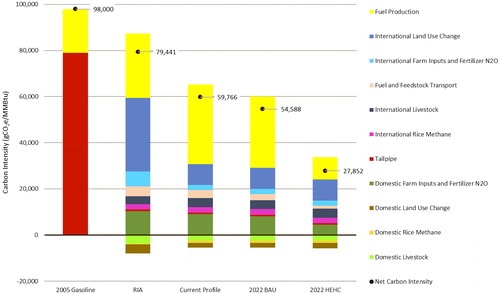
In the RIA, EPA quantified the LCA emissions associated with its ‘average’ 2005 gasoline (see note 1) at 98,000 g CO₂e/MMBtu. For corn ethanol, the RIA projected emissions in 2022 at 79,441 g CO₂e/MMBtu. The ethanol is produced at a new natural gas-powered dry mill refinery, with a fractionation process in place for extracting corn oil, and producing a DGS mix that is 63% dry and 37% wet. Interestingly, the projected emissions for corn ethanol fall just short of the 20% reduction required in the RFS2 to qualify as a renewable fuel. EPA assumed there would be additional emissions reductions by 2022 related to increased efficiencies (e.g. in drying DGS). With these efficiency gains, EPA projected the life-cycle GHG emissions of corn ethanol in 2022 at 21% lower than gasoline.

Our current conditions scenario assesses the life-cycle emissions of corn ethanol at 59,766 g CO₂e/MMBtu. This is a 39% reduction in GHG emissions relative to gasoline; almost twice the reduction developed in the RIA. This scenario assumes ethanol plants use a composite process fuel that reflects today’s mix of natural gas, coal, and other fuels used by refineries. The 39% reduction is the industry-wide average GHG reduction for corn ethanol relative to gasoline. However, most refineries today use natural gas as a process fuel. In Table A2, replacing the fuel production emissions in the current conditions scenario with the fuel production emissions in the BAU scenario indicates that the GHG profile of corn ethanol produced in these refineries is 42.6% lower than that of gasoline.

Our BAU scenario assumes a continuation through 2022 of current trends in average corn yields per hectare, process fuel switching from coal to natural gas, and increasing fuel efficiency in heavy-duty trucks. Based on these trends, we project life-cycle GHG emissions for corn ethanol in 2022 at 54,588 g CO₂e/MMBtu. This scenario indicates that even if the ethanol industry does not act to reduce emissions, the GHG profile of corn ethanol will continue to improve. By 2022, the emissions associated with producing and combusting corn ethanol will be, on average, 44.3% lower than the emissions associated with producing and combusting gasoline.

Our HEHC scenario assumes refineries actively reduce their GHG profile. Refineries use sustainably produced biomass as the process fuel, contract with farmers to grow corn using low-emissions practices, and locate CAFOs near refineries. Projected emissions for corn ethanol in 2022 are 27,852 g CO₂e/MMBtu, which is a 71.6% reduction in GHG emissions relative to gasoline. The main source of emissions reductions is the shift to sustainable biomass as the process fuel. While it is not likely the ethanol industry as a whole will undertake these changes, it does highlight the emissions reductions that are technically possible with currently available technologies. Given an appropriate incentive, some refineries will likely undertake these changes. The most likely source of such an incentive are opportunities to participate in new or expanding markets for low-carbon transportation fuels. As noted at the beginning of this paper, a number of these markets are now taking shape outside of the United States.

Finally, in the HEHC scenario refineries achieve an emissions reduction of 4021 g CO₂e/MMBtu by contracting with farmers to grow corn using low-emissions technologies and practices. The practices considered in this scenario are currently available and in use to some degree. Again, given an appropriate incentive, refineries could use such contracts to reduce ethanol’s current GHG profile. Subtracting 4021 g CO₂e/MMBtu from the current emissions levels of a ‘representative’ refinery results in an emissions profile 43.1% lower than that of gasoline. For natural gas-powered refineries, the emissions reduction would be 46.7%.

Conclusions

This paper assesses the current greenhouse gas profile of US corn ethanol and two projected emissions profiles for 2022. The starting point is the GHG life-cycle analysis done by the US Environmental Protection Agency in 2010 for US corn ethanol as part of its Regulatory Impact Analysis (RIA) for the Revised Renewable Fuel Standard (RFS2). In the RIA, EPA projected that in 2022, the life-cycle emissions associated with ethanol would be 21% lower than those of an energy-equivalent quantity of gasoline.

We assess each of the 11 emissions categories in the 2010 EPA LCA in light of new data, technical papers, research studies and other information that have become available since 2010. Aggregated across the 11 categories, we find US corn ethanol is developing along an emissions pathway significantly lower than what EPA projected in 2010. Our analysis indicates the current GHG profile of US corn ethanol is, on average, 39% lower than that of gasoline. For natural gas-powered refineries, this value is almost 43% lower. Finally, current trends in the ethanol industry and actions refineries could take to reduce emissions offer opportunities to lower the GHG profile of corn ethanol to between 47.0 and 70.0% relative to gasoline.

Our analysis is timely because many countries (e.g. Colombia, Japan, Brazil, Canada and the European Union) are now developing or revising their renewable energy policies. These policies typically require biofuel substitutes for gasoline to reduce GHG emissions by more than 21%. Our results could help position US corn ethanol to compete in these new and growing markets.

Disclosure statement

No potential conflict of interest was reported by the authors.

Notes

Notes

1 The US gasoline supply consists of gasolines imported from many foreign regions and gasolines refined domestically from petroleum extracted from numerous domestic and foreign regions. The gasoline assessed in the RIA is a composite product constructed to represent the ‘average’ gasoline consumed in the United States in 2005 [1, section 2.5].

2 To help readers quickly compare the methods of the RIA and our study, Appendix Table A1 identifies key differences in data, models, emission factors and other information used in the two studies by emissions source category.

3 To make our results familiar to a wider set of people in other disciplines, Appendix Table A2 presents emissions by source category for the RIA and our three scenarios in both g CO₂e/MMBtu and g CO₂e/MJ.

4 The regional breakdown, in acres, is in Rosenfeld et al. [5; table 2-6, p. 18].

5 ARMS is an annual survey that collects data on the financial condition, production practices, and resource use for US farms. Each ARMS samples about 5000 fields and 30,000 farms that are representative of that year’s surveyed commodities.

6 For example, in Appalachia, 95.2% of acres apply nitrogen (N) and the average application rate is 173.01 kg/ha. Multiplying the adoption rate by the application rate gives an effective N application rate across the region of 164.70 kg/ha.

7 Our approach allows us to clearly distinguish between new acres brought into corn production due to increases in ethanol production, acres leaving corn production due to increases in supply of distiller grains and solubles, and the GHG impacts related to each set of acres (i.e. changes in emissions related to changes in farm input use and changes in soil carbon). Additionally, our approach allows us to account for the increase in average corn yields per hectare since 2010.

8 This table is reproduced in Rosenfeld et al. [5, p. 82].

9 MOVES estimates emissions for mobile sources covering a broad range of pollutants, and allows multiple-scale analysis.

10 The term ‘sustainably produced biomass’ abstracts from several emissions-related issues that could accompany a large-scale increase in the use of biomass as a process fuel by ethanol refineries. For example, LUC and farm input emissions could change if large areas of land are shifted into energy crop production. The nature and GHG intensity of feedstock production geared to supply large quantities of biomass to the ethanol industry would likely vary by region, and even by refinery location. While an analysis is beyond the scope of this paper, we acknowledge that our HEHC scenario is likely a relatively low-emissions case.

Appendix Table A1. Summary of Key Data Sources and Models Used in the Regulatory Impact Analysis (RIA) Life Cycle Analysis and the Current Greenhouse Gas (GHG) Profile.

Source category	RIA [1]	Current GHG profile
General – Global warming potentials (GWPs)	Second Assessment Report (1996) • Methane: 21 • Nitrous oxide: 310	Fourth Assessment Report (2007) • Methane: 25 • Nitrous oxide: 298
Domestic farm inputs and fertilizer Nitrous Oxide (N2O)	• Fertilizer application rates and fuel Consumption: Forestry and Agricultural Sectoral Optimization Model (FASOM version 2010)  • Fertilizer and fuel production Emission factors: The Greenhouse Gas, Regulated Emissions, and Energy Use in Transportation Model (GREET) version 2009  • Fertilizer use emission factors: Daily Century (DAYCENT) Model (version 2010)	• Fertilizer application rates: [6]  • Fuel consumption: [7]  • Fertilizer and fuel production emission factors: GREET (version) 2015  • Fertilizer use emission factors:[10]  • Animal feed co-product credit: GREET (version 2015)
Domestic land use	• Acres: FASOM (version 2010)  • Emission factors: DAYCENT Model (version 2010)	• Acres: [12]  • Emission rates: Century and Cole Models (version 2015)
Domestic rice methane	• Acres: FASOM (version 2010)  • Emission factors: [19]	• Acres: same as [1]  • Emission factors: [21]
Domestic livestock	• Change in livestock populations: FASOM (version 2010)  • Emission factors: [19]	• Change in livestock populations: same as [1] except poultry  • Livestock conventional feed emission Factors: [21] • Emission reductions from Distillers Grains with Solubles as feed: GREET (version 2015)
International livestock	• Populations: Food and Agriculture Policy Research Institute-Center for Agricultural and Rural Development (FAPRI-CARD) (version 2010)  • Emission Factors: [10]	• Populations: same as [1]  • Emission factors: [10] except for Canada (2016) with a country-specific update
International land-use change	• Acres: FAPRI-CARD (version 2010)  • Emission factors: Winrock International (2009)	• Acres: [12]; in two scenarios, acres adjusted with data in [17]  • Emission factors: Winrock International (2009), Woods Hole (2010) and California Air Resources Board (CARB) Agricultural - Ecological Zones (AEZ) (2015)
International farm inputs and fertilizer N2O	• Acres and production: FAPRI-CARD (version 2010)  • Fertilizer application rates: [30] and [31, version 2009]  • Fuel use: [34]  • Fertilizer and fuel production emission factors: GREET (version 2009) • Fertilizer use emission factors: Methodology similar to domestic	• Acres and production: [12]  • Fertilizer application rates: [31, version 2015]  • Fuel use: same as [1]  • Fertilizer and fuel production emission Factors: GREET (version 2015) • Fertilizer use emission factors: [10]
International rice methane	• Acres: FAPRI-CARD (2010)  • Emission factors: [10]	• Acres: same as [1]  • Emission factors: same as [1]
Fuel and feedstock transport	• Transport distances: GREET (version 2009) • Emission factors: GREET (version 2009)	• Transport distances: GREET (version 2015) • Emission factors: GREET (version 2015)
Fuel production	• Process energy: GREET (version 2009) • Emission factors: GREET (version 2009)	• Process energy: GREET (version 2015) • Emission factors: GREET (version 2015)
Tailpipe	• Emissions: [39]	• Emissions: GREET (version 2015)

Appendix Table A2. Emissions by scenario and category.

	Estimated Greenhouse Gas (GHG) emissions (in grams carbon dioxide equivalent per million British thermal units)
Emissions category	RIA (2010)	Current	2022 BAU	2022 HEHC
Domestic farm inputs	10,313	9065	8190	4490
Domestic Land Use Change	−4000	−2038	−2038	−2359
Domestic rice methane	−209	−1013	−1013	−1013
Domestic livestock	−3746	−2463	−2463	−2463
International Land Use Change	31,790	9094	9094	9094
International farm inputs	6601	2217	2217	2217
International rice methane	2089	2482	2482	2482
International livestock	3458	3894	3894	3894
Fuel and feedstock transport	4265	3432	2641	1237
Fuel production	28,000	34,518	31,006	9695
Tailpipe	880	578	578	578
Total	79,441	59,766	54,588	27,852
	Estimated GHG emissions (in grams carbon dioxide equivalent per Mega Joule)
Domestic farm inputs	9.77	8.59	7.76	4.26
Domestic Land Use Change	−3.79	−1.93	−1.93	−2.24
Domestic rice methane	−0.20	−0.96	−0.96	−0.96
Domestic livestock	−3.55	−2.33	−2.33	−2.33
International Land Use Change	30.13	8.62	8.62	8.62
International farm inputs	6.26	2.10	2.10	2.10
International rice methane	1.98	2.35	2.35	2.35
International livestock	3.28	3.69	3.69	3.69
Fuel and feedstock transport	4.04	3.25	2.50	1.17
Fuel production	26.54	32.72	29.39	9.19
Tailpipe	0.83	0.55	0.55	0.55
Total	75.30	56.65	51.74	26.40

References

- U.S. Environmental; Protection Agency (EPA). 2010. Renewable Fuel Standard Program Regulatory Impact Analysis. EPA-420-r-10-006. February 2010.
- Searchinger T, Heimlich R, Houghton RA, et al. Use of Cropland for Biofuels Increases Greenhouse Gases Through Emissions from Land-Use Change. Science. 2008; 319:1238–1240.
- Energy Information Agency (EIA). Annual Energy Outlook for 2007: With Projections to 2030. U.S. Department of Energy. 2006. DOE/EIA-0383(2007). February.
- Adams D, Alig R, McCarl BA, et al. FASOMGHG Conceptual Structure and Specification: Documentation. 2005. Retrieved from http://agecon2.tamu.edu/people/faculty/mccarl-bruce/papers/1212FASOMGHG_doc.pdf
- Rosenfeld J, Lewandrowski J, et al. A Life-Cycle Analysis of the Greenhouse Gas Emissions from Corn-Based Ethanol. Report prepared by ICF under USDA Contract No. AG-3142-D-17-0161. September 05, 2018.
- Economic Research Service (ERS). Agricultural Resource Management Survey. U.S. Department of Agriculture. 2013. http://www.ers.usda.gov/dat-products/arms-farm-financial-and-crop-production-practices.aspx
- University of Tennessee. Field Crop Budgets For 2015. E12-4115: 2015. University of Tennessee Institute of Agriculture. http://economics.ag.utk.edu/budgets/2015/Crops/2015CropBudgets.pdf
- Argonne National Laboratory (ANL). 2015. GREET 1_2015. https://greet.es.anl.gov/greet_1_series
- Weidema BP, Bauer C, Hischier R, et al. The ecoinvent database: Overview and methodology, Data quality guideline for the ecoinvent database version 3. 2013. www.ecoinvent.org
- IPCC. 2006 IPCC Guidelines for National Greenhouse Gas Inventories. National Greenhouse Gas Inventories Programme, 2006. Eggleston H.S., Buendia L., Miwa K., Ngara T. and Japan: IGES.
- Dunn JB, Mueller S, Qin Z, et al. Carbon Calculator for Land Use Change from Biofuels Production (CLUB). Argonne National Laboratory (ANL). Argonne. 2014.
- Taheripour F, Tyner WE. Biofuels and land use change: Applying recent evidence to model estimates. Applied Sciences. 2013;3:14–38.
- Taheripour F, Tyner WE, Wang MQ. Global land use change due to the U.S. cellulosic biofuels program simulated with the GTAP model. 2011. Available at http://greet.es.anl.gov/publication-luc_ethanol.
- Wright C, Wimberly C. Recent land use change in the Western Corn Belt threatens grasslands and wetlands. Proc Natl Acad Sci USA.. 2013;110:4134–4139.
- Lark TJ, Salmo JM, Gibbs HH. Cropland expansion outpaces agricultural and biofuel policies in the United States. Env. Res. Letters. 2015; 10: 1-11. DOI: 10.1088/1748-9326/10/4/044003.
- Wright CB, Larson T, Lark H, et al. Recent grassland losses are concentrated around U.S. ethanol refineries. Environmental Research Letters. 2017; 12, 1-16. DOI: 10.1088/1748-9326/aa6446.
- Babcock BA, Fabiosa JF. The Impact of Ethanol Subsidies on Corn Prices: Revisiting History. Center for Agricultural and Rural Development. Iowa State University. 2011. CARD Policy Brief 11-PB5.
- Dunn JB, Merz D, Copenhaver KL, et al. Measured extent of agricultural expansion depends on analysis technique. Biofuels, Bioprod Bioref.. 2017;11:247–257. DOI: 10.1002/bbb
- EPA. Inventory of U.S. Greenhouse Gas Emissions and Sinks: 1990-2003. 2005. EPA 430-R-05-003. Retrieved from http://www3.epa.gov/climatechange/Downloads/ghgemissions/05CR.pdf
- United States Department of Agriculture (USDA). U.S. Agriculture and Forestry Greenhouse Gas Inventory: 1990-2013. 2016. Office of the Chief Economist. Climate Change Program Office. Technical Bulletin No. 1943.
- EPA. U.S. Environmental Protection Agency. 2016. EPA 430-R-16-002. http://www.ethanolproducer.com/plants/listplants/US/
- Renewable Fuels Association. 2018. http://www.ethanolrfa.org/resources/industry/co-products/#1456865649440-ae77f947-734a.
- MODIS. (n.d.). MODIS/Terra Land Cover Type Yearly L3 Global 1km SIN GRID (MOD12Q1) Version 4.
- Friedl M. 2009. Validation of the Consistent-Year V003 MODIS Land Cover Product, MODIS Land Team Internal PI Document. December 2009. Retrieved from http://landval.gsfc.nasa.gov/Results.php?TitleID=mod12_valsup1.
- Dunn J, Mueller S, Kwon HY, et al. Land-use change and greenhouse gas emissions from corn and cellulosic ethanol. Biotechnol Biofuels. 2013;6:51.
- Babcock BA, Iqbal Z. Using Recent Land Use Changes to Validate Land Use Change Models. Staff Report 14-SR 109. Center for Agricultural and Rural Development: Iowa State University. 2014. http://www.card.iastate.edu/publications/dbs/pdffiles/14sr109.pdf
- CARB. Staff Report: Calculating Carbon Intensity Values from Indirect Land Use Change and Crop Based Biofuels. Appendix I: Detailed Analysis for Indirect Land Use Change. 2015. http://www.arb.ca.gov/regact/2015/lcfs2015/lcfs15appi.pdf
- Taheripour F, Zhao X, Tyner WE. The impact of considering land intensification and updated data on biofuels land use change and emissions estimates. Biotechnol Biofuels. 2017;10:191. DOI: 10.1186/s13068-017-0877-y.
- CARB. Proposed Regulation to Implement the Low Carbon Fuel Standard. Staff Report: Initial Statement of Reasons. 2009. https://www.arb.ca.gov/regact/2009/lcfs09/lcfsisor1.pdf
- Heffer P. Assessment of Fertilizer Use by Crop at the Global Level, 2006/07 - 2007/08. 2009. Paris, France: International Fertilizer Industry Association.
- Food and Agriculture Organization (FAO). FAOSatat. FAO, Statistics Division. 2018. http:/faostat3.fao.org/homeE
- ERS. China Agricultural and Economic Data: National Data Results. 2009. Retrieved from http://www.ers.usda.gov/Data/China/NationalResults.aspx?DataType=6&DataItem=160&Str Datatype=Agricultural±inputs&ReportType=0
- EPA. RFS2 FRM modified version of GREET1.8c Upstream Emissions Spreadsheet. 2009. October 30.
- International Energy Agency (IEA). International Energy Agency Data Services. 2015. Retrieved from http://wds.iea.org/WDS/Common/Login/login.aspx
- International Rice Research Institute (IRRI). (2008, October 15). International Rice Research Institute. Retrieved from www.irri.org
- Cai H, Burnham A, Wang M, et al. The GREET Model Expansion for Well-to-Wheels Analysis of Heavy-Duty Vehicles. 2015. https://greet.es.anl.gov/publication-heavy-duty
- Oak Ridge National Laboratory. Analysis of Fuel Ethanol Transportation Activity and Potential Distribution Constraints. 2009. DOI: 10.3141/2168-16
- EIA. Corn Ethanol Yields Continue to Improve. U.S Energy Information Administration. 2015. May. http://www.eia.gov/todayinenergy/detail.cfm?id=21212.
- EPA. NMIM and MOVES Runs for RFS2 Air Quality Modeling: Memorandum. United States Environmental Protection Agency. Washington, D.C. 2010.
- Washington Department of Ecology, 2016. Greenhouse Gas Reporting: Transportation Fuel Suppliers. http://www.ecy.wa.gov/programs/air/permit_register/ghg/GHG_transp.html
- California ARB, 2015. CA-GREET 2.0 Model. http://www.arb.ca.gov/fuels/lcfs/ca-greet/ca-greet.htm
- USDA. 2016. USDA Agricultural Projections to 2025. USDA Agricultural Projections No. (OCE-2016-1) 99 pp, February 2016.
- Trenkel ME. Slow- and Controlled-Release and Stabilized Fertilizers: An Option for Enhancing Nutrient Use Efficiency in Agriculture. 2010. International Fertilizer Industry Association.
- LookChem. 2008. Nitrapyrin. http://www.lookchem.com/Nitrapyrin/
- Boland S, Unnasch S. Carbon Intensity of Marginal Petroleum and Corn Ethanol Fuels. Life Cycle Associates Report. 2014. LCA.6075.83.2014, Prepared for Renewable Fuels Association.