Application of extension rings in thermography for electronic circuits imaging

ABSTRACT

Thermographic cameras are often used in areas, where resolutions below 100 µm per pixel are required, as for example in electronics. Such resolutions can be obtained using dedicated lenses. As an alternative, some manufacturers are offering extension rings to be added between the lens and the camera housing, to increase the final image spatial resolution. To test the latter solution and its impact on thermographic temperature measurements, a set of aluminium extension rings was manufactured and mounted in different combinations between an InSb cooled thermographic camera and its lens. Next, the camera, a blackbody IR source, a thick-film resistor on alumina substrate, a microscope reticle calibration glass, and two integrated test circuits were used to investigate the impact of the rings on the temperature measurement accuracy and the achieved spatial resolution. It was demonstrated, that extension rings are a very useful tool in thermography, as long as their impact on the measurement system is taken into account, considering numerical aperture reduction, rings heating by the operating camera, and the cold stop related vignetting. The impact will greatly depend on the specific design of the camera to be used and its lens configuration.

KEYWORDS:

• Extension ring
• spatial resolution
• thermography
• electronics

1. Introduction

Thermographic measurements are often requiring imaging with resolutions below 100 µm per pixel. For this purpose, dedicated and expensive microscopic lens assemblies can be utilised [1–4]. As an alternative, some manufacturers are offering extension rings. If the camera design allows it, it is also possible for the user to design and manufacture such rings on his own, implementing a quick and low-cost solution. Extension rings have been used for thermographic measurements in electronics [5–8], non-destructive testing (NDT) and materials research [9–14] or biology and medicine [15,16]. In most cases extension rings provided by the camera manufacturer were used.

Whereas extension rings are a solution well known and described in visible light macrophotography, little has been published specifically on their use in thermography, their advantages, drawbacks, limits, and precautions to be taken during their use. In [8] the authors proposed an infrared thermography protocol for 40 µm spatial resolution quantitative microelectronic imaging, where an increased spatial resolution was obtained with the help of a 30 mm long extension ring mounted between a cooled InSb camera and its lens. The authors used contact pads and micro-resistors to evaluate the resolution provided by their setup. In [17] the authors used 4 different extension rings, mounted in combinations, to measure the temperature of a reference blackbody source and to demonstrate ring length impact on image magnification and temperature measurement accuracy. The possibility of the rings being heated by the operating camera was also suggested.

This paper is divided into six main sections. In the second one, the theoretical impact of extension rings on image magnification is presented. The third section is dedicated to the diffraction limit problem. The measurement setup is described in the fourth section, whereas the measurement results are analysed in the fifth section. Conclusions are presented in the sixth section.

2. Theoretical impact of extension rings on image magnification

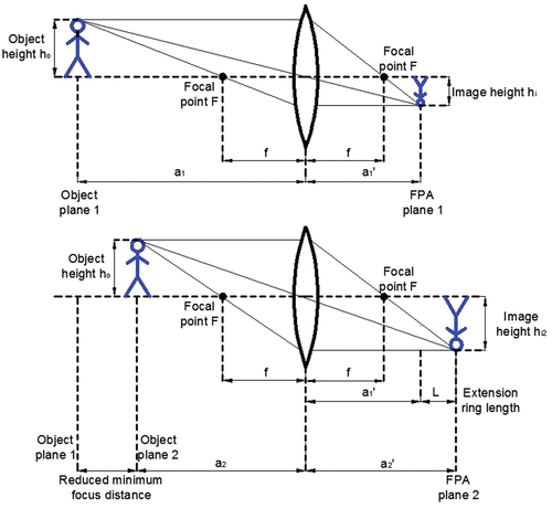
Adding an extension ring between the camera lens and the Focal Plane Array (FPA) modifies the optical setup configuration of the camera, as shown in Figure 1.

Figure 1. Impact of an extension ring on the optical setup of a camera and image magnification.

Assuming a thin lens approximation, for the configuration without extension ring, the Gaussian lens equation gives:

(1) $\frac{1}{a_1}+\frac{1}{{a_1}^{\prime }}=\frac{1}{f}$(1)

where a₁ is the lens to object distance, a₁’ is the lens to image distance, and f is the lens focal length. The magnification ratio can be expressed using Equation (2)(2) $m_1=\frac{h_i}{h_o}$(2) :

(2) $m_1=\frac{h_i}{h_o}$(2)

where h_i is the image height and h_o is the object height. Adding an extension ring modifies the optical system, which can be described using Equation (3)(3) $\frac{1}{a_2}+\frac{1}{{a_2}^{\prime }}=\frac{1}{f}$(3) and (4(4) $m_2=\frac{{\mathit{h}}_{\mathit{i}2}}{h_o}=m_1+\frac{L}{f}$(4) ):

(3) $\frac{1}{a_2}+\frac{1}{{a_2}^{\prime }}=\frac{1}{f}$(3)

(4) $m_2=\frac{{\mathit{h}}_{\mathit{i}2}}{h_o}=m_1+\frac{L}{f}$(4)

where h_i2 is the image height for the configuration with a ring added and L is the ring length.

3. Diffraction limit

An important element to be considered when using extension rings in a thermographic camera is the diffraction-related resolution limit. Depending on the distances between the radiation source, the aperture, the imaging plane, and the dimensions of the aperture, far-field Fraunhofer diffraction patterns, near-field Fresnel patterns or Fresnel-Fraunhofer transition region patterns, having a different width compared to the dimension of the original aperture, can be observed [18–21]. These phenomena may result in a different spatial resolution limit. Usually, when imaging distant objects through a lens, Fraunhofer approximation is taken into account, giving at the focal plane of the lens a circular pattern, known as the Airy disc, and a resolution limit that can be described using Equation (5)(5) $D_{\mathit{Airy}}=2.44\mathit{\lambda N}$(5) :

(5) $D_{\mathit{Airy}}=2.44\mathit{\lambda N}$(5)

where D_Airy is the diameter of the first dark ring in the pattern, λ is the incident radiation wavelength, and N the f-number of the lens focused at infinity. In a configuration where extension rings are added, this equation is no longer valid, since the imaged object has to be placed close to the lens and the optics focal imaging plane is also moved, as shown in Figure 1. In such a case Equation (6)(6) $D_{\mathit{Airy}}=2.44\mathit{\lambda N}\frac{\left(m_2+1\right)}{\left(m_1+1\right)}$(6) should be used:

(6) $D_{\mathit{Airy}}=2.44\mathit{\lambda N}\frac{\left(m_2+1\right)}{\left(m_1+1\right)}$(6)

where m₁ is the magnification of the lens without any extension ring and m₂ is the magnification of the system with an extension ring, and the (m₂ +1)/(m₁ +1) term is used to calculate the so-called working f-number when imaging an object placed closer than at infinity [22].

In [19], the authors presented an extensive review of criteria to distinguish between Fraunhofer and Fresnel diffraction, proposed in different publications, clearly demonstrating the lack of full agreement on the subject in the literature. For this reason, knowing also that the camera used for our experiments had a minimum focusing distance of 30 cm, reduced to below 3 cm when mounting on the longest extension ring setup prepared, and because no data regarding the exact design of the camera lens was available, no preliminary assumption regarding the type of expected diffraction pattern was made before the experiments.

4. Measurement setup

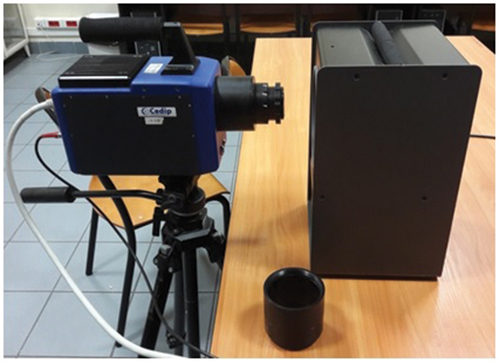
A Cedip Titanium 560 M cooled thermographic camera with an InSb Focal Plane Array (FPA), a 640 × 512 pixel resolution and 15 µm pixel pitch was used for tests. The camera was equipped with a standard 50 mm (focal length), F/2 (f-number) lens. That choice was made for two reasons: lens mount using a standard metric thread M80, allowing for easy extension ring manufacturing and mounting, and camera software giving full access to its configuration, including user temperature calibration and non-uniformity correction (NUC) procedures. The camera was distributed by the manufacturer with a single 1/2” = 12.7 mm long, black anodised aluminium extension ring. Three additional black anodized aluminum extension rings were manufactured, two 30 mm long and one 60 mm long. For clarity, the 10 possible camera ring configurations were numbered from R0 (no ring) to R9 (132.7 mm long ring composed of the complete set of the four rings). The rings are shown in Figure 2 and the measurement setup is presented in Figure 3.

Figure 2. Set of extension rings used during experiments; from the left: 12.7 mm, 30 mm, 30 mm and 60 mm ring.

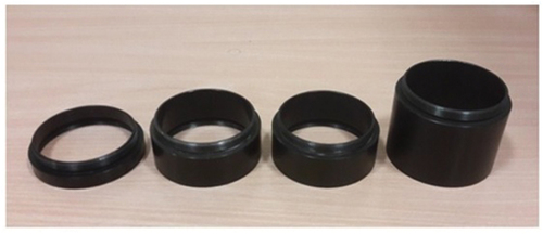
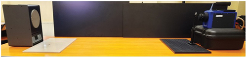
Figure 3. Setup used to evaluate the impact of different combinations of extension rings on the temperature measurement accuracy and image spatial resolution; a Cedip Titanium 560 M camera (shown with the 60 mm ring) and a Fluke 4181 IR calibrator.

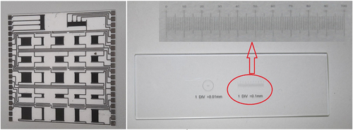
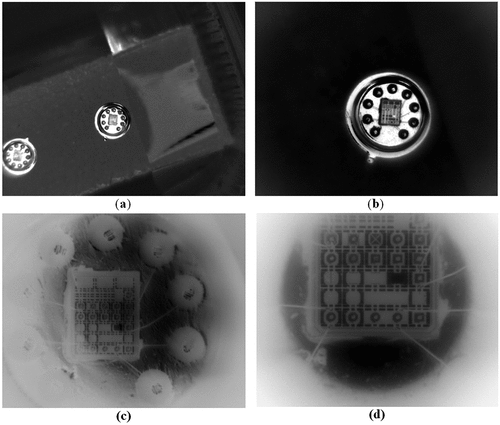
For each ring combination, the camera was used to measure the temperature of a blackbody, for three different temperature setpoint values: ambient (24.1°C), 50°C and 75°C. A Fluke 4181 IR calibrator was used as the blackbody. For each temperature and ring configuration, a horizontal temperature profile across the entire thermogram was recorded, the spatial resolution per pixel was calculated and the camera focusing distance was measured. Because the uniform surface of the blackbody made it difficult to focus the camera, as no reference points were visible, a custom-made thick-film test resistor network on alumina was used for correct focusing (Figure 4). For spatial resolution measurements, a microscope reticle calibration slide ruler was used. The ruler was placed in a holder, in front of the camera, and next, it was illuminated with a small halogen lamp. The metallic overprint on the glass substrate provided the required thermal contrast. The resolution was calculated as the quotient of the horizontal distance seen by the camera and the number of pixels. A perfect lens without any aberrations was assumed and, at first, the limits imposed by diffraction phenomena were not taken into account. The pictures of the thick-film resistor and the ruler are shown in Figure 4.

Figure 4. The thick-film resistor network on alumina (left) and the microscope reticle calibration slide ruler (0.1 mm/division and 0.01 mm/division) (right) used for camera focus setting and spatial resolution measurements.

To experimentally assess the spatial resolution limits of the tested camera setup with different extension ring configurations, taking into account the diffraction phenomena, two additional series of measurements were made. First, the blackbody temperature was measured through a Thorlabs VA100C/M adjustable 0–6 mm micrometric slit inserted between the camera and the blackbody, changing the slit width from fully open to fully closed. Horizontal slit temperature patterns were recorded and compared to the slit width. To provide enough temperature contrast between the VA100C/M body and the radiation passing through the slit for narrow settings, the blackbody temperature was set to 150°C. As shown in Figure 5, the blackbody was placed 150 cm from the slit to avoid its heating by the blackbody during measurements.

Figure 5. The camera spatial resolution measurement setup – blackbody temperature measured through a Thorlabs VA100C/M adjustable 0–6 mm micrometric slit.

The second series of measurements consisted in imaging an integrated test circuit containing a series of chip-level interconnects and spiral inductors of known dimensions. The chip layout was compared with the thermograms obtained for different ring configurations.

5. Measurement results

5.1. Ring impact on temperature measurement accuracy

The goal of the first series of measurements was to verify the impact of adding extension rings between the camera lens and camera body on temperature measurement accuracy. For all 10 ring configurations – from R0 to R9 – the camera was used to measure the blackbody temperature for 24.1°C (ambient), 50°C and 75°C setpoints. To guarantee the correct measurement results, a non-uniformity correction procedure (NUC) was performed for the camera without any extension ring, using the camera software. Next, for each subsequent ring configuration and blackbody temperature setting, a thermogram was recorded, from which a horizontal temperature profile was extracted at half-height of the image. The measurements were made in quick succession, first setting the temperature and next increasing, step by step, the total length of the extension ring. The resulting set of profiles for ambient blackbody temperature is shown in Figure 6. In Figure 7 the profiles obtained for 75°C are shown. The profiles for 50°C were similar to the 75°C case and thus, were not included in the article.

Figure 6. Temperature measured across blackbody surface for different extension ring length (blackbody temperature set to the ambient = 24.1°C); R0 = no ring; R9 = 132.7 mm ring.

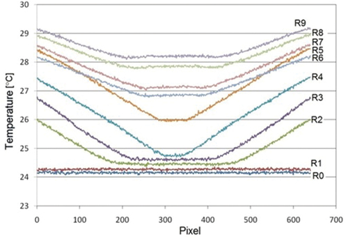
Figure 7. Temperature measured across blackbody surface for different extension ring length (blackbody temperature set to 75°C); R0 = no ring; R9 = 132.7 mm ring.

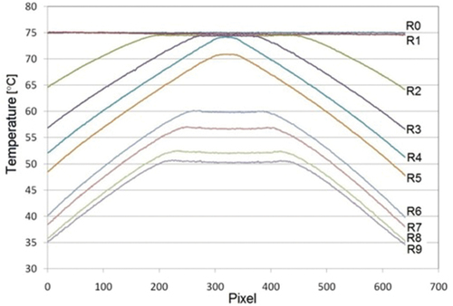
For the 75°C blackbody setting, a strong vignetting was observed. The longer the ring was, the stronger that effect was. The temperature measurement was correct in the central area of the image, around the optical axis of the camera. The increase of the ring length decreased the radius of the correct temperature measurement disc, and beyond ring R4 (60 mm long), further ring length increase led to measured temperature underestimation. There are several causes to that. First, reducing the distance between the imaged object from a₁ to a₂ (see Figure 1), which is a result of adding a ring, increases the intensity of radiation by (a₁/a₂)², based on the inverse square law. Second, the increase of magnification of the imaged object from m₁ to m₂ in both the X and Y axis reduces the intensity of the radiation from that object reaching the lens by (m₁/m₂)². Combining those two effects gives an f-number increase given by Equation (7)(7) $\frac{{\mathit{N}}_{\mathit{ring}}}{N_{\mathit{no}\mathit{ring}}}=\frac{\left(m_2+1\right)}{\left(m_1+1\right)}$(7) [22]:

(7) $\frac{{\mathit{N}}_{\mathit{ring}}}{N_{\mathit{no}\mathit{ring}}}=\frac{\left(m_2+1\right)}{\left(m_1+1\right)}$(7)

where N_{no ring} is the camera lens f-number for the configuration without any extension ring and N_ring is the working f-number of the camera lens with a ring added. This proportionality coefficient was already used in Equation (6)(6) $D_{\mathit{Airy}}=2.44\mathit{\lambda N}\frac{\left(m_2+1\right)}{\left(m_1+1\right)}$(6) for Airy disc diameter calculation.

A cooled thermographic camera was used for the experiments; an inherent design element of these cameras is a cold shield, usually matching the lens f-number. Based on Figure 1, if such additional aperture is present in the optical axis of the imaging system, and an extension ring is added between the lens and the camera housing, effectively magnifying the image, a vignetting effect will appear.

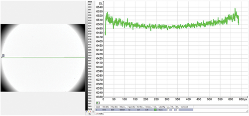
To confirm that hypothesis, a 2-point NUC procedure was made for the camera with rings. The results for the 90 mm ring are shown in Figure 8. As presented, even if it was possible to reduce vignetting, the shadow created by the cold shield remained.

Figure 8. Blackbody image after a 2-point NUC and its temperature profile (in digital units) for the camera with a 90 mm extension ring.

As an additional confirmation of the cold shield problem, a microbolometer FLIR E95 uncooled camera, thus a design without a cold shield, was used. Because of the camera design and its lens short back focal distance, a 4 mm ring was enough to obtain a visible image magnification, whereas reducing the system focusing distance to about 1 cm, making such configuration barely useful for practical applications. No vignetting was observed, thus confirming the problem of the cold shield encountered in the cooled camera.

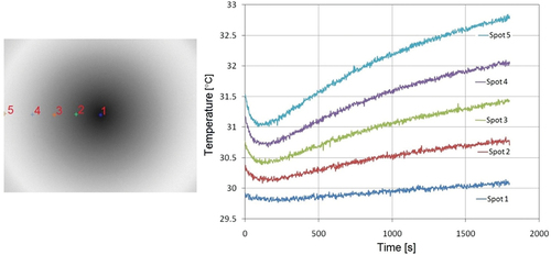
For the ambient temperature blackbody setting, the temperature measurement was again correct in the central area of the image, around the optical axis of the camera (Figure 6). The increase the ring length decreased the radius of the correct temperature measurement disc. Beyond ring R4 (60 mm long), further ring length increase led to measured temperature overestimation increasing with ring length. Also, for all but the shortest 12.7 mm ring, instead of vignetting, an inverse effect was observed: a temperature rise when moving away from the camera optical axis. It was assumed that this temperature rise was caused by the radiation coming from the rings being gradually heated by the operating camera. To verify this hypothesis, the R4 ring was placed for 10 min inside a fridge, quickly mounted on the camera, and next, the blackbody temperature set to the ambient (29.9°C during this experiment) was recorded for 30 min. The results are shown in Figure 9.

Figure 9. Temperature measured for 30 minutes in 5 different spots of the blackbody surface using the 60 mm extension ring (blackbody temperature set to the ambient = 29.9°C).

To confirm those results and the ring heating hypothesis, an additional 60 mm ring was printed using PLA material (Polylactic acid), and the previous measurement was repeated without cooling, while the measurement time was extended to 1 h. The results of that measurements are shown in Figure 10.

Figure 10. Temperature measured for 60 min in 5 different spots of the blackbody surface using a 60 mm extension ring printed from PLA.

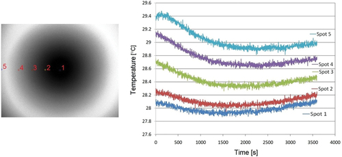
The thermal conductivity of aluminium is 205 W/m*K, three orders of magnitude higher than PLA (0.25 W/m*K), thus, as shown in Figure 10, the process of ring heating by the operating camera not only was much slower, but also the temperature changes within a 1 h period were an order of magnitude smaller than for the aluminum ring. It clearly indicates that low thermal conductivity materials should be used for extension ring manufacturing or the measurement time should be limited. If possible, a ring temperature control system could be added.

5.2. Spatial resolution measurements

The next step was the measurement of spatial resolution that could be obtained using the tested camera with extension rings. First, the spatial resolution calculated as the quotient of the horizontal distance seen by the camera and the number of pixels, neglecting lens aberrations and diffraction, was measured. A microscope reticle calibration slide ruler was placed in a holder in front of the camera, and illuminated with a small halogen lamp. The metallic overprint on glass substrate provided adequate thermal contrast. The results are shown in Table 1. An example of thermogram obtained during those experiments is shown in Figure 11.

Figure 11. Measurement of the camera spatial resolution for the R5 ring configuration (72.7 mm).

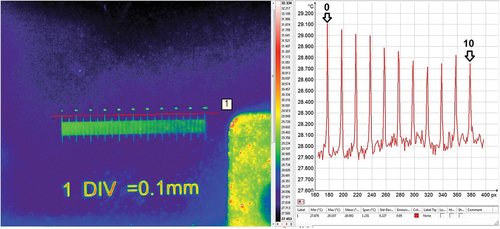
Table 1. Spatial resolution for different extension ring configurations.

Extension ring	R0	R1	R2	R3	R4	R5	R6	R7	R8	R9
Total ring length [mm]	0	12.7	30	42.7	60	72.7	90	102.7	120	132.7
Measured resolution (slide ruler) [µm/pixel]	90	50	25	18.5	12	10.5	8	7	6	5.5
Magnification measured (slide ruler)	0.17	0.3	0.6	0.81	1.25	1.43	1.87	2.14	2.5	2.72
Magnification calculated (Equation. 4(4) $m_2=\frac{{\mathit{h}}_{\mathit{i}2}}{h_o}=m_1+\frac{L}{f}$(4) )	0.17	0.42	0.67	1.02	1.37	1.62	1.97	2.22	2.57	2.82
Expected Airy disk diameter Dairy (Equation. 6(6) $D_{\mathit{Airy}}=2.44\mathit{\lambda N}\frac{\left(m_2+1\right)}{\left(m_1+1\right)}$(6) ) [µm]	28.55	31.72	39.04	44.16	54.9	59.3	70.03	76.61	85.4	90.77
Focusing distance [cm]	30	21.5	10.8	7.5	5.5	4.5	3.9	3.5	3.0	2.7

For the camera without any extension ring and the minimum focusing distance given by the manufacturer, i.e. 30 cm, a resolution of 90 µm per pixel was obtained. As the camera’s FPA pixel pitch was 15 µm, it gave a magnification of 0.17. For configurations with an extension ring from, R1 to R9, a resolution from 50 µm/pixel to 5.5 µm/pixel was obtained (no diffraction taken into account) and magnification from 0.3 to 2.72 was achieved. The measured magnifications were compared with the values calculated using Equation (4)(4) $m_2=\frac{{\mathit{h}}_{\mathit{i}2}}{h_o}=m_1+\frac{L}{f}$(4) , giving comparable results. It must be emphasised that for each of those measurements, because of the weight and the size of the camera, and the need to change the rings, the measurement setup had to be remade each time and the camera lens refocused. Thus, repeating the measurements with a different position of the lens focusing ring would give slightly different resolution values, especially for shorter rings, when larger values of depth of focus were possible. The measured spatial resolutions were compared with the Airy disk diameters calculated based on Equation (6)(6) $D_{\mathit{Airy}}=2.44\mathit{\lambda N}\frac{\left(m_2+1\right)}{\left(m_1+1\right)}$(6) , using λ = 4 µm as wavelength. For all but R0 and R1 configurations, the Airy disk diameter was higher than the measured geometrical resolution, thus suggesting that those configurations could be diffraction limited.

To further investigate the problem of diffraction limit, for the R9 ring configuration, the blackbody temperature was measured through a Thorlabs VA100C/M adjustable 0–6 mm micrometric slit inserted between the camera and the blackbody, changing the slit width from fully open to fully closed. Slit horizontal temperature patterns were recorded and compared to the set slit width. Since gradually closing the slit considerably reduced the amount of infrared energy reaching the FPA, the temperature of the blackbody was set to 150°C. The results obtained for a 500 µm, 200 µm, 50 µm, and 20 µm slit are shown in Figure 12.

Figure 12. Blackbody temperature profile (150°C) imaged through(a) 500 µm, (b) 200 µm, (c) 50 µm and (d) 20 µm wide slit using the R9 extension ring configuration (132.7 mm).

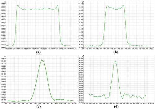
For the 500 µm slit, a temperature profile with an almost vertical temperature rise was obtained, typical for the geometric approximation region [18–21], with diffraction patterns visible on the edges of the slit. Closing the slit gradually changed the shape of the temperature profile across the slit, getting finally for the 20 µm opening an unexpected pattern, as shown in Figure 12(d), with a visible single peak.

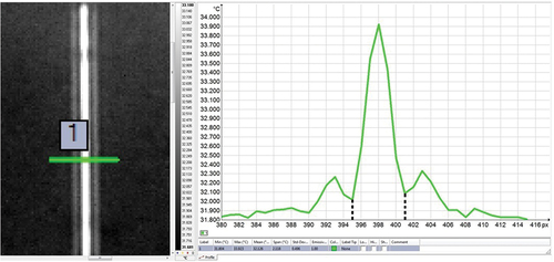
In optical imaging, there is a clear distinction between the light reaching the camera through the slit and no light zone created by the slit. In the case of thermal imaging, both the slit and its body, having an ambient temperature, are a source of thermal radiation. Thus, some diffraction patterns could be masked by the slit body’s own radiation. To solve the problem, the blackbody temperature was raised to 250°C and the 20 µm slit temperature profile was reacquired. The result is shown in Figure 13. A dominant central peak with sidebands is visible, with a temperature drop between them, but to a level higher than the slit body temperature. Based on the spatial resolution for the R9 ring configuration from Table 1, the slit visible on the thermogram was 6 pixels wide (dashed vertical lines in Figure 13), equivalent to 33 µm, much below the calculated Airy disc diameter from Table 1. The pattern from Figure 13 clearly differs from a classical Airy disk pattern and is typical for the Fresnel-Fraunhofer transition region [18–21], thus a better resolution than expected was obtained. Those results are in accordance with the analysis presented in [23] for a slit-lens system diffraction patterns.

Figure 13. Blackbody temperature profile (250°C) imaged through a 20 µm wide slit using the R9 extension ring configuration (132.7 mm);dashed vertical lines were used for diffraction pattern width measurement.

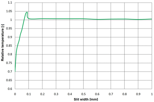
Based on the slit temperature measurements, a slit response function for the R9 ring was created and is shown in Figure 14. For this research, the X axis of the drawing was scaled in mm of the slit opening instead of typical angle values. The Y curve value was calculated as the blackbody temperature measured through the slit, at its centre, normalised to the temperature for the fully opened slit. The temperature increase observed on the drawing for the slit narrower than 100 µm was caused by the diffraction patterns seen at the edge of the slit and shown in Figure 12(a,b).

Figure 14. Thermogram of the blackbody set to 150°C imaged through a 20 µm wide slit using the R9 extension ring configuration (132.7 mm).

The final experiments related to the camera spatial resolution consisted in imaging an integrated test circuit containing elements of known dimensions. The thermograms of the circuit obtained for different ring lengths are shown in Figure 15. Based on the data from Table 1, an approximately 16x magnification was obtained for the R9 ring configuration, compared to a no-ring setup.

Figure 15. Thermograms of the test circuit (2 mm x 3 mm); a) camera without extension ring; b) camera with a 30 mm extension ring; c) camera with a 90 mm extension ring; d) camera with a 132.7 mm extension ring.

To measure the diffraction limited spatial resolution of the camera with rings mounted on, two circuit elements were chosen, an octagonal spiral inductor and a single 12 µm wide interconnect Figure 16. After careful consideration, the approach suggested in [8], that is, heating an element on the circuit surface was rejected, as this would create an inevitable temperature gradient. Instead, it was decided to perform the measurements at room temperature.

Figure 16. Layout of an integrated spiral inductor and integrated interconnect used for resolution tests as dimensions reference.

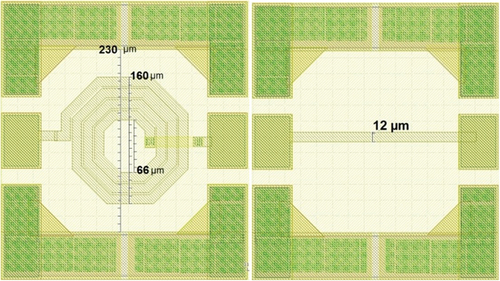
The layout-based diameter of the spiral inductor (160 µm) and the interconnect width (12 µm) were compared to the dimensions visible on the thermogram. The distance measurements based on the temperature profiles were taken between the peaks of the temperature on both sides of each structure. These peaks represented the temperature of the silicon substrate. It was anticipated that this approach would lead to the overestimation of the sizes, as there will be inevitably metal-silicon transition pixels at the edges of each of the tested structures. Examples of the measurements for the R9 ring configuration for the spiral inductor and the integrated interconnect, respectively, are shown in Figures 17 and 18. For clarity, the thermograms are presented in the pixel mode. The dashed vertical lines in Figures 17 and 18 are showing the edges of the spiral and the interconnect, as used for their dimensions estimations, based on the thermograms. The obtained results are shown in Table 2.

Figure 17. Thermogram of the integrated spiral inductor obtained using the R9 extension ring configuration (132.7 mm) and the temperature profile across the inductor; dashed vertical lines were used for spiral diameter measurement.

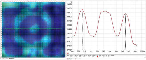
Figure 18. Thermogram of the integrated interconnect obtained using the R9 extension ring configuration (132.7 mm) and the temperature profile across the interconnect; dashed vertical lines were used for interconnect width measurement.

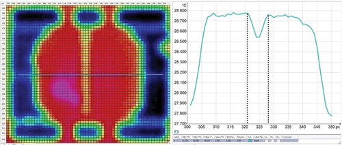
Table 2. Spiral inductor and integrated interconnect dimensions measurement results.

Extension ring	none	R2	R4	R1+R2 +R4	R2+R3 +R4	R1+R2 +R3+R4
Total ring length [mm]	0	30	60	90	120	132.7
Measured resolution (slide ruler) [µm/pixel] (from Table 1)	90	25	12	8	6	5.5
Spiral inductor diameter (based on circuit layout) [µm]	160	160	160	160	160	160
Measured spiral inductor diameter (based on thermogram) [µm]	-^(1)	190	207	184	195	194
Test interconnect width (based on circuit layout) [µm]	12	12	12	12	12	12
Test interconnect width (based on thermogram) [µm]	-^(1)	-^(1)	46	48	45	40

^aElement invisible on the thermogram or too small to be measured.

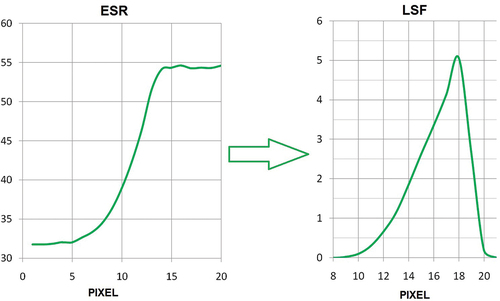
For the camera configuration with the 132.7 mm extension ring (R9), based on temperature profiles obtained for the adjustable slit and test circuit geometries measurements, the spatial resolution of the system was evaluated using the edge response method [24–29]. It consisted in measuring the temperature across a thermal edge, obtaining the Edge Step Response (ESR), and differentiating ESR curve to obtain the Line Spread Function (LSF) (Figure 19). The resolution was the full width at half maximum (FWHM) of the LSF curve. An integer value of 5 pixels was obtained, corresponding, according to the data from Table 1, to 27.5 µm. It must be noted that it was still possible to see on the thermograms of the test circuit a separate 12 µm wide integrated interconnect.

Figure 19. System resolution measurement based on its Edge Step Response (ESR) and Line Spread Function (LSF) curve.

5.3. Lens defocusing – super-resolution experiment

Though there is not any unambiguous definition of the ‘super-resolution’ term, it is often described by the authors as a group of solutions for enhancing imaging resolution beyond what is achievable based on traditional far-field Fraunhofer diffraction and Rayleigh or Sparrow resolution criteria [30,31]. One of the techniques described in the literature consists in using specific aperture geometries during imaging, to obtain diffraction patterns with a narrower central peak at the expense of larger sidebands. Examples of such apertures can be found in [32], where the authors described an annular aperture and an apodized one.

In the experiments involving the adjustable slit described in the previous section, during focus adjustments before the measurements, different diffraction patterns were observed. This phenomenon led to the question, whether defocusing the camera lens and using one of such patterns could improve spatial resolution.

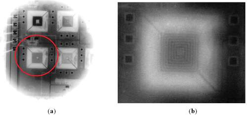
As object for the experiments, a second semiconductor test circuit containing six square spiral inductors was used. Each of the inductors had a 9 µm interconnect width and a 9 µm edged to edge distance between successive turns. The circuit was made in a standard silicon technology and in MEMS version, where the semiconductor substrate below the suspended spirals was removed. The thermogram of one of the spiral inductors acquired with the camera with the R9 extension ring, correctly focused at the surface of the semiconductor die, is shown in Figure 20(a). Although the external outline of the inductor was clearly visible, it was impossible to distinguish the exact spiral geometry. A uniform surface was visible. Next, when the lens was focused at a plane about 300 µm below the circuit surface, the thermogram shown in Figure 20(b) was obtained. The successive turns of the spiral became visible, clearly demonstrating resolution improvement. Similar results were obtained for both the MEMS and standard technology test circuit.

Figure 20. Thermogram of a MEMS test circuit containing suspended spiral inductors obtained using the R9 extension ring configuration (132.7 mm); (a) camera focused at the circuit surface; (b) camera focused approximately 300 µm below the circuit surface.

6. Conclusions

Extension rings are an easy solution for spatial resolution increase (image magnification) when using thermographic cameras. Whereas the results that could be obtained using them and the problems to be faced will depend greatly on the specific design of a given camera and its lens configuration, there are some general conclusions that can be drawn based on the research presented in the previous sections of this paper.

• The magnification obtained by adding an extension ring can be easily calculated using Equation (4)(4) $m_2=\frac{{\mathit{h}}_{\mathit{i}2}}{h_o}=m_1+\frac{L}{f}$(4) .

• Adding an extension ring will change the f-number of the camera optical system. The change can be estimated by using Equation (7)(7) $\frac{{\mathit{N}}_{\mathit{ring}}}{N_{\mathit{no}\mathit{ring}}}=\frac{\left(m_2+1\right)}{\left(m_1+1\right)}$(7) .

• If a cooled thermographic camera with an extension ring is used, the vignetting caused by the camera cold stop must be taken into account. This problem did not occur with the tested uncooled microbolometer camera.

• Depending on the camera design and the applied ring length, the process of ring heating by the operating camera may have to be taken into account. In such a case it will be preferable to manufacture the rings from a low thermal conductivity material or to add a ring temperature control system.

• If a cooled thermographic camera with and extension ring is used, both effects – vignetting and ring thermal radiation – are present simultaneously. Depending on the temperature of the imaged object compared to the ambient temperature and the ring temperature, one of those effects may become dominant.

• Based on the variable slit diffraction patterns measurements, a spatial resolution equivalent to 27.5 µm was achieved for the camera with the 132.7 mm ring mounted on.

• It was demonstrated, that when imaging a semiconductor test circuit, defocusing the tested camera lens, that is, setting the focus at a plane other than the circuit surface, allowed to increase the system spatial resolution. It was possible to image an integrated spiral inductor with a 9 µm trace width and a 9 µm turns separation. Further investigation of that phenomenon is planned.

• Before using any rings for thermal imaging or temperature measurements, their impact on the camera temperature measurement must be verified. A NUC and user calibration procedure could be required.

Disclosure statement

No potential conflict of interest was reported by the author(s).

References

- Montanini R, Scimone T, De Caro S, et al. Full-frame infrared thermal imaging of power electronics devices by means of multiple time-delayed measurements. Quant Infrared Thermogr J. 2015;12(2):149–161.
- Ryu M, Romano M, Batsale JC, et al. Microscale spectroscopic thermal imaging of n-alkanes. Quant Infrared Thermogr J. 2016;13(2): 154–163.
- Aladov A, Chernyakov A, Zakgeim A. Infrared micro-thermography of high-power AlIngan LEDs using high emissivity (black) in IR and transparent in the visible spectral region coating. Quant Infrared Thermogr J. 2019;16(2): 172–180.
- Breitenstein O, Sturm S. Lock-in thermography for analyzing solar cells and failure analysis in other electronic components. Quant Infrared Thermogr J. 2019;16(3–4): 203–217.
- Kaminski A, Nichiporuk O, Jouglar J, et al. Application of infrared thermography to the characterization of multicrystalline silicon solar cells. Proceedings 5th International Conference on Quantitative InfraRed Thermography - QIRT; 2000 July 18-21; Reims, France.
- Kałuża M, De Mey BWG, Hatzopoulos A, et al. Thermal impedance measurement of integrated inductors on bulk silicon substrate. Microelectron Reliab. 2017;73:54–59.
- Papagiannopoulos I, Chatziathanasiou V, Hatzopoulos A, et al. Thermal analysis of integrated spiral inductors. Infrared Phys Technol. 2013;56:80–84.
- Boué C, Fournier D. Cost-effective infrared thermography protocol for 40μm spatial resolution quantitative microelectronic imaging. Infrared Phys Technol. 2006;48(2):122–129.
- Koruba P, Reiner J, Zakrzewski A. Detection of cracks in laser deposited coatings by laser spot thermography. Proceedings 13th International Conference on Quantitative InfraRed Thermography - QIRT; 2016 July 4-8; Gdansk, Poland.
- Komisarczyk A, Dziworska G, Krucinska I, et al. Visualisation of Liquid Flow Phenomena in Textiles Applied as a Wound Dressing. Autex Res J. 2013;13(4):141–149.
- Gorostegui-Colinas E, Muniategui A, López de Uralde P, et al. A novel Automatic Defect Detection Method for Electron Beam Welded Inconel 718 components using Inductive Thermography. Proceedings 14th International Conference on Quantitative InfraRed Thermography - QIRT; 2018 June 25–29; Berlin, Germany.
- Carlomagno GC. Some Thermographic Measurements in Complex Fluid Flows. J Flow Visualization Image Process. 2010;17(1):15–40.
- Taram A, Roquelet C, Meilland P, et al. Nondestructive testing of resistance spot welds using eddy current thermography. Appl Opt. 2018;57(18):63–68.
- Goff MR, Clark RP. Computerised Infra-Red Thermography in Medicine and Physiology. J Photographic Sci. 1985;33(2):60–67.
- Lane B, Moylan S, Whitenton EP, et al. Thermographic measurements of the commercial laser powder bed fusion process at NIST. Rapid Prototyping J. 2016;22(5):778–787.
- Stabentheiner A, Kovac H, Hetz SK, et al. Assessing honeybee and wasp thermoregulation and energetics - New insights by combination of flow-through respirometry with infrared thermography. Thermochim Acta. 2012;534:77–86.
- Kałuża M, Więcek B, De Mey G. The use of extension tubes in thermography. Proceedings 10th International Conference on Quantitative InfraRed Thermography - QIRT; 2010 July 27-30; Québec, Canada
- Hecht E. Optics. 5th ed. Pearson Global Editions; 2017; pp. 460–462. section 10.1.2
- Medina FF, Garcia-Sucerquia J, Castaneda R, et al. Angular criterion to distinguish between Fraunhofer and Fresnel diffraction. Optik. 2004;115:547–552.
- Davidović M, Božić M. Geometrical, Fresnel, and Fraunhofer Regimes of Single-Slit Diffraction. Phys Teach. 2019;57:176–178.
- Panuski CL, Mungan CE. Single-Slit Diffraction: transitioning from Geometric Optics to the Fraunhofer Regime. Phys Teach. 2016;54:356–359.
- Extension Tubes and Effective f-stops. ReefNet Inc; 2002.
- Wenzel RG, Telle JM, Carlsten JL. Fresnel diffraction in an optical system containing lenses. J Opt Soc Am A. 1986;3:838–842.
- Offroy M, Roggo Y, Milanfar P, et al. Infrared chemical imaging: spatial resolution evaluation and super-resolution concept. Anal Chim Acta. 2010;674:220–226.
- Offroy M, Roggo Y, Duponchel L. Increasing the spatial resolution of near infrared chemical images (NIR-CI): the super-resolution paradigm applied to pharmaceutical products. Chemometr Intell Lab Syst. 2012;117:183–188.
- Levenson E, Lerch P, Martin M. Infrared imaging: synchrotrons vs. arrays, resolution vs. speed. Infrared Phys Technol. 2006;49:45–52.
- Alshweikh AM, Kusminarto K, Suparta G. An Improved Method of Measuring Spatial Resolution of the Computed Tomography from ESF based on CT phantom images. Int J Appl Eng Res. 2018;13:12318–12325.
- Lashansky S, Mansbach S, Berger M, et al. Edge response revisited. SPIE Proceedings, vol. 6941, Infrared Imaging Systems: Design, Analysis, Modeling, and Testing XIX; 2008. pp. 1–9. DOI:10.1117/12.777957
- Jeong-Heon S, Dong-Han L, Sun-Gu L, et al. Modulation Transfer Function (MTF) Measurement for 1 m High Resolution Satellite Images such as KOMPSAT-2 Using Edge Function. Proceedings of the Korean Society of Remote Sensing Conference; 2005. pp. 482–484.
- Borlinghaus RT. Super-Resolution. On a Heuristic Point of View About the Resolution of a Light Microscope. Technological Readings. Leica Microsystems; 2014 Dec.
- Lasch P, Naumann D. Spatial resolution in infrared microspectroscopic imaging of tissues. Biochim Biophys Acta. 2006;1758:814–829.
- Mazneva AA, Wright OB. Upholding the diffraction limit in the focusing of light and sound. Wave Motion. 2017;68:182–189.