Scanning inductive pulse phase thermography with changing scanning speed for non-destructive testing

ABSTRACT

This work aims at non-destructive detection of surface and subsurface defects in metallic specimens (e.g. railway track components) via pulsed inductive thermography in a moving setup. A new approach for scanning with changing speed has been developed to enable manual scanning of components in track. A steel specimen is heated with an inductor, and the surface temperature, including its variation over time, is recorded with an infrared camera. The infrared sequence is evaluated by Fourier transform to phase image, in order to increase the image quality. The proposed method uses a referencing object with AprilTags visible in each frame, allowing an adjustment by image registration. Changes in velocity during the scanning process are possible, as demonstrated by a manually performed scan of the specimen and the corresponding evaluation. Results obtained with different infrared cameras and scanning speeds were condensed into an estimation of the maximum scanning speed for a given camera specification.

KEYWORDS:

• Inductive thermography
• image registration
• scanning
• defect detection
• rolling contact fatigue

1. Introduction

Inductive thermography is a well-established method for non-destructive testing of surface defects in metallic specimen. Excited with a short eddy current pulse (0.1–1 s) the surface layer of a specimen is first heated for 1–5°C and temperature changes on the surface during and after the pulse are recorded via infrared camera. Surface defects influence the eddy current flow and therefore the resulting temperature distribution [1–6]. By pixel-wise Fourier transform of the recorded image sequence a phase image is calculated in order to evaluate the specimen for surface defects. As the phase image implies temperature changes of the entire sequence, it reduces effects of inhomogeneous heating and inhomogeneous surface properties [7]. This evaluation method not only has the benefit of increasing the quality of results, but it also allows the localisation and characterisation of the surface defects. Disturbances in the temperature distribution caused by surface defects can be seen in the phase image as the phase values change in correlation with depth and penetration angle of the defects [1].

Inductive scanning pulse phase thermography (SPPT) is used for non-destructive testing of long specimen. Excitation, applying a constant inductive power, heats the specimen’s surface, while either the specimen or the inductor is moving relative to each other. The infrared camera records temperature changes in a fixed distance behind the inductor. Evaluation to a phase image is possible for this type of measurement, but an additional step is needed, where the recorded image sequence is reorganised according to the used scanning speed to eliminate the movement in the sequence [8].

SPPT is performed with constant speed so that shifts between frames can be calculated with knowledge of motion speed and spatial resolution (px/mm) of the infrared camera. On the other hand, when the motion speed cannot be measured exactly, the frames will get reorganised incorrectly. In this work a method for image registration via AprilTags [9] is used to track movement in each frame of the recorded image sequence. During the scan a registration target with AprilTags is also recorded along with the specimen. Thus, information about the movement is included in the recorded images. Furthermore, this new approach allows the reorganisation for evaluation even if the movement speed varies during the scan, since each frame is shifted individually. This means that manual scanning pulse phase thermography on specimen can be performed with the proposed method.

In the following sections our approach for the new scanning method is presented. The next section describes the setup used in laboratory including test rigs, the used specimen as well as the registration target. Section 3 then explains the process of evaluating scanning measurements with varying speeds. The measurements and results performed on the presented specimen are shown in Section 4, and in the last section the new method will be briefly summarised and discussed.

2. Laboratory setup

2.1. Test rigs

Two test rigs with different inductor types are used for the measurements presented in this paper. In both cases the infrared camera IRCam VELOX 1310k SM was used for recording the image sequences. This cooled quantum detector camera with an Indium Antimonide semiconductor material has a frame rate of 180 Hz at full frame. However, measurements in this work were performed in binning mode, which reduces the resolution and allows frame rates up to 594 Hz [10]. Measurements with an uncooled µ-bolometer camera (FLIR A615) were also carried out for the detection of surface defects. The goal was to investigate if this method is also suited for uncooled µ-bolometer cameras, because they are cheaper, smaller in size, more robust and therefore better suited for some mobile applications. Table 1 presents a comparison of both used cameras and the used settings, like spectral range, frame rate, noise equivalent temperature difference (NETD) and integration time (IT) and thermal time constant (TC), respectively.

Table 1. Data of the used camera systems [10,11].

Camera	Technology	Spectral range [µm]	Resolution [px × px]	Frame rate [Hz]	IT, TC [ms]	NETD [mK]
IRCam VELOX 1310k SM	Quantum detector	1.5–5.5	1280 × 1024	180	0.5	20
IRCam VELOX 1310k SM	Quantum detector	1.5–5.5	640 × 512	594	0.5	20
FLIR A615	µ-bolometer	7.5–14	640 × 480	50	8	50
FLIR A615	µbolometer	7.5–14	640 × 240	100	8	50

The first test rig, shown in Figure 1a, uses a line heating source. Since this inductor is water-cooled, the inductor can be switched on for as long as the cooling of the coil is sufficient and the specimen can be heated continuously during the measurement. A linear table, controlled via programmable logic controller (PLC), is used to move the specimen with speeds up to 0.2 m/s. During the measurements the linear table can be moved not only by a constant motion speed, but different acceleration and deceleration values can be set in the control software to modify the scanning speed. At this test rig the specimen is first heated by the inductor and the camera records the cooling of the specimen after it passes the inductor.

Figure 1. a.) Test rig for scanning with an inductive linear heating source; b.) Test rig for scanning with a U-shaped inductor; c.) U-shaped inductor in close-up.

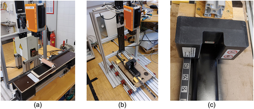
The second test rig uses an air-cooled, U-shaped inductor with a ferritic core and copper windings. In this setup a continuous heating during the whole scanning procedure is not possible, due to overheating of the copper wiring in the inductor. However, short pulses of 0.5 s duration can be repeated with a short cooling break of at least 0.02 s between heating pulses. A specimen is placed on a platform with wheels running on two rails (see Figure 1b). The platform is either pushed or pulled manually or moved with constant speed by connecting the platform to the PLC-controlled linear table. The inductor itself is designed in such a way that the region between the arms of the inductor is in view of the camera (see Figure 1c). In this case, the heating of the specimen in the field of the inductor and the subsequent cooling are evaluated together.

2.2. Description of specimens

One specimen with subsurface defects and one specimen with surface defects were tested with the new method. Due to their shiny metallic surfaces both specimens were spray-painted with a matte black colour, to reduce influences from reflections and to increase emissivity. Both specimens are ferromagnetic steel.

A specimen with flat bottom holes (FBH) was tested on the test rig with linear inductor. The 200 × 100 × 6 mm³ large metallic plate has 12 drilled flat bottom holes with different diameters and depths (see Figure 2a) and was previously used in Ref [8]. During measurement the side with the FBHs is placed downwards and the undamaged side without holes faces towards inductor and camera, so that the holes appear as subsurface defects in the evaluation.

Figure 2. a.) Sketch of the flat bottom hole sample [8]; b.) Image (bottom view) of the sample with flat bottom holes.

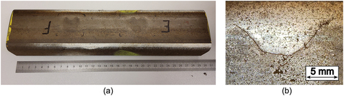
The second inspected specimen is a 300 mm long pearlitic rail head with small surface cracks and two larger squats (see Figure 3a). This specimen was tested on the test rig with the U-shaped inductor. The squats on this specimen can be seen with the naked eye (Figure 3b), but the cracks are not or just barely visible. Squats are a common damage type in railway components caused by rolling contact fatigue [12]. On the surface both cracks and squats run parallel to the gauge corner, but the crack propagates underneath the surface at a shallow angle towards the centre of the railhead [13].

Figure 3. a.) Rail piece with squats and small cracks; b.) Close-up of one squat on the rail piece sample.

2.3. Description of the registration target

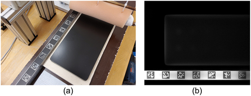
As the motion speed during the measurement is changing and not known, the proposed solution is to determine the shifting from the recorded images themselves. Along the inspected specimen a calibration target is recorded, which is used to register the motion and to calculate the shifting between the recorded frames. To register the movement in the recorded images so called AprilTags are used. These visual fiducials are commonly used in robotics and photogrammetry and are highly optimised for their automatic detection and localisation in images. Different types of these AprilTags, so called families, are freely available. The main distinguishing features of various families are the number of bits encoded in a single AprilTag and the minimum hamming distance, which is an indicator of diversity between AprilTags of a specific family [9]. In our case, the AprilTags were produced on a spray-painted metallic ruler by removing the paint at the tags location with an industrial laser. Figure 4a shows the resulting painted ruler with metallic 15 × 15 mm² AprilTags in a distance of 15 mm in between. The used AprilTags belong to the family 36h11 which means that 36 bits are encoded in one AprilTag and the minimum hamming distance is 11. Each of the 20 AprilTags along a distance of 585 mm on the ruler is different. In the infrared spectrum the tags appear darker due to lower emissivity of the metallic surface. In Figure 4b the infrared image after heating the specimen and the calibration target is shown.

Figure 4. a.) Specimen and ruler with AprilTags on the linear table; b.) View of the specimen and the AprilTags in the infrared image.

3. Description of the evaluation workflow of scanning with changing motion speed

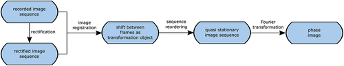
In this section the developed workflow is described by the example of a measurement carried out at the test rig with linear heating source. During the heating the specimen is accelerated up to a speed of 40 mm/s and then decelerated until it stops outside of the camera’s field of view. This results in a scanning image sequence of the specimen with varying motion. The workflow described in Figure 5 shows the necessary steps needed for the evaluation of this image sequence. Image rectification on the entire sequence is performed in order to correct the camera distortion; this step is described in more detail in Ref [14]. The main contribution of the current paper is the registration process, which is used to recognise the changing speed in the images.

Figure 5. Workflow for evaluating the image sequence.

3.1. Image registration

Image registration is performed either on the recorded image sequence or on the rectified image sequence. Rectification is only necessary if a perspectivity of the camera view or a distortion of the optics is not negligible. The goal of the image registration step is to compute a transformation object, containing the pixel shift in consecutive frames due to the movement during the scanning process. To increase the speed of this algorithm, the pixel shift between two image frames with a chosen time distance is computed and the pixel shifts for intermediate frames are obtained by linear fitting. As an example, Figure 6 compares the frame number 801 and the frame number 821 of the rectified sequence. Since just the AprilTags on the ruler are used for registration, only this region of interest (ROI) is selected for further comparison (see Figure 6(a,c)). In the next step image processing methods are used to binarize these ROIs through edge detection and to delete unwanted small spots by applying morphological operators. This results in a black and white contour image of the AprilTags (see Figure 6(b,d)). Next, phase correlation is applied on these binary images to compute shifts between the images. The specimen and the registration target are aligned in the setup in such a way that only the displacement along the direction of movement has to be considered. In Figure 6 a shift of 10 pixels between both considered images of frame 801 and 821 can be observed.

Figure 6. Images used for registration via phase correlation; a.) ROI in frame No. 801; b.) Binarized ROI of frame No. 801; c.) ROI in frame No. 821; d.) Binarized ROI of frame No. 821.

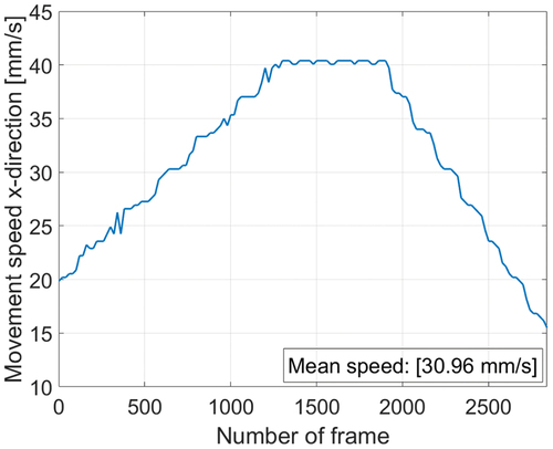
Using the spatial resolution in the camera’s field of view (in the current case 0.34 mm/px), the shift in pixels can be transformed to a shift in millimetre. The moving speed in mm/sec is determined using the camera’s known frame rate, here 200 Hz. As it is shown in Figure 7., the average speed of this experiment is 31 mm/s with velocities from 15 mm/s up to 40 mm/s. The pixel shifts between the images are stored in transformation objects, which are used in the next step to compute a quasi-stationary image sequence of the inspected object.

Figure 7. Current speed calculated using the camera’s frame rate.

3.2. Sequence reordering

To evaluate temperature changes at a certain point of the specimen surface, the movement of the specimen has to be taken into account. The proposed method in this work is to reorganise the whole image sequence to a quasi-stationary sequence using the previously calculated pixel shifts. In this new sequence both calibration target and specimen appear stationary while inductor and camera appear moving over the specimen. To achieve this quasi-stationary sequence first an empty sequence is prepared which can fit all original images including their directional shift. Therefore, the image format of this new empty sequence is increased with respect to the original sequence to consider this shift. Figure 8 shows three original images which are positioned in this new sequence according to the calculated shift. In each frame of the newly generated sequence only a portion of a frame is filled with actual image data, while the rest stays empty. To reduce the size of this figure only the lower halves of the images with the referencing object are depicted in Figure 8.

Figure 8. Lower half of shifted images with the referencing object containing the AprilTags; a.) Frame at the beginning of the recorded sequence; b.) Frame at the middle of the recorded sequence; c.) Frame at the end of the recorded sequence.

3.3. Fourier transform

As next step from the quasi-stationary image sequence a phase image is calculated by applying a pixel-wise Fourier transform of the sequence. Since each frame of this generated sequence has pixels with no real image data (see the black pixels in Figure 8), these pixels with a value of zero are ignored for the Fourier transform. The resulting phase image is depicted in Figure 9.

Figure 9. Phase image of the specimen with flat bottom holes and the AprilTags used for registration.

4. Measurements and results

4.1. Specimen with flat bottom holes

The measurements for the specimen with flat bottom holes were performed with scanning speeds of approximately 10 to 40 mm/s. The excitation frequency of the induction heating was 100 kHz. In this case in ferromagnetic steel sample the eddy current penetration depth is about 0.05 mm. Due to the Joule heating generated in the thin layer below the top surface, the heat flows into the sample. Since the flat bottom holes are located at various depths, the heat is reflected after different time delay. A mean speed of 31 mm/s is selected, in order to be able to observe this postponed response from the flat bottoms in different depths.

To reduce the data, the infrared sequence was recorded with a frame rate of 200 Hz instead of 594 Hz. The resulting phase image of a measurement with changing scanning speed is shown in Figure 9. It is to mention that due to the variation in speed the evaluation time of different regions also varies. In the case of Figure 9 for pixels at the left and right sides of the specimen approximately 1200 frames with temperature data are available for calculating phase values. This means cooling of the specimen is evaluated for a time period of 6 s in these areas. At the middle of the specimen the available number of frames decreases to approximately 1000 due to the higher motion speed, which means that only 5 s of cooling is evaluated in this region.

4.2. Rail piece with squats and cracks

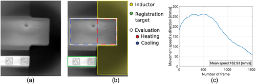
In the case of subsurface defects, as e.g. the FBHs, it is enough to record the surface temperature after the heating, as the cool down function of the temperature reveals the hidden defects. On the other hand, for surface defects the most relevant information occurs already during the inductive heating pulse [14]. Therefore, the measurements on the rail head were performed using the test rig with the U-shaped inductor, as this one also allows recording the surface temperature during the heating. For scanning, as it is shown in Ref [14], the pulse duration is estimated as the time a specific point on the specimen surface is moved inside the inductor’s electromagnetic field. The experiment was carried out by pulling the platform manually. Multiple pulses of 0.5 s with an excitation frequency of 60 kHz and breaks of 0.02 s between the heating pulses were used to heat the specimen as uniformly as possible. Penetration depth of the eddy current in the rail head for this excitation frequency is about 0.06 mm. The infrared camera’s frame rate was set to 594 Hz and the camera’s spatial resolution was 0.24 mm/px. Figure 10a shows one frame of the recorded sequence, and Figure 10b shows the same frame with an overlay of ROIs: the yellow area marks the U-shaped inductor which blocks a large area in the camera’s field of view. Therefore, two ROIs are picked for evaluation. The green region contains the AprilTags and it is used for referencing the images. The white area in Figure 10b is used for evaluation of the phase image of the specimen and has a size of 402 × 205 pixels. It is assumed that heating of the specimen occurs only between the arms of the inductor (region marked in red). Cooling of the specimen occurs after the specimen passes the inductor, indicated by the blue area. For evaluation a cooling area, which is 1.5 times longer than the heating area is considered. Evaluations with different ratios have shown that the chosen ratio of 1.5 between heating and cooling area resulted in phase images with a good contrast between cracks and sound surface for this particular setup. Reducing this ratio also reduces the number of pixels evaluated, which increases noise in the resulting phase image. On the other hand, increasing the ratio reduces the contrast in the result, as cooling around a crack occurs quickly. Figure 10c shows that the platform was pulled with motion speeds between 50 and 260 mm/s. For this experiment the same evaluation steps are carried out, as described previously for the sample with the FBHs.

Figure 10. a.) Original frame of the recorded sequence; b.) Explanation of ROIs inside the recorded sequence c.) Calculated speed for manually pulling the inspection platform.

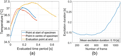
The varying speed influences how long a position at the specimen is heated in the inductor’s magnetic field. The diagram in Figure 11a shows temperature curves for three different points at the specimen in the quasi-static image sequence. Due to the acceleration at the start (blue line in the diagram) and the beginning deceleration at the middle of the recorded sequence (red line in the diagram), the evaluation time periods as well as the excitation duration for these two points are in similar range. However, further deceleration at the end of the recording increases evaluation and excitation duration (yellow line in the diagram). An approximation for the excitation duration is calculated by dividing the width of the used inductor by the calculated motion speed at a certain time period. In Figure 11b the estimated excitation duration is depicted, calculated for an inductor width of 36 mm. It is to see that at the start, the first part of the specimen entering the inductor’s field is heated approximately for 0.15 s and at the end of the scan the heating duration is increasing up to 0.30 s.

Figure 11. a.) Temperature-time diagram of three different points in the quasi-static image sequence; b.) Calculated excitation duration for an inductor width of 36 mm while specimen is inside the inductors field.

The calculated phase image of this experiment is depicted in Figure 12, and it shows that both squats and the shallow short cracks along a line can be excellently detected and located via manual scanning. Since the inductor is not water-cooled, to avoid the risk of its overheating, continuous heating cannot be applied. As mentioned before in section 2.1, heating pulses of 0.5 s duration with pauses of 0.02 s are used in this measurement. Due to this necessary pulsing the calculated phase values differ from one evaluated column to another. To achieve a seamless result, the scaling of phase values in each column was adjusted to fit the scaling of the previous column. The resulting phase image shows the detected cracks as short bright lines; the two squats are surrounded by darker areas which indicate propagation of the squats beneath the surface. It is to note that the goal is to detect defects, due to their different phase values from the defect-free background. In each column of the phase image this detection is possible, as in each column the defect and the defect-free region during the motion through the inductor’s magnetic field are heated in the same way, but they cause different phase values. On the other hand, due to the different pulse heating and phase-shift, in each column the phase image has a different value. For the defect detection only the difference between the defect-free background and the defect is relevant; therefore, the adjustment of the scaling from one column to the next one was introduced. In this way the phase of the defect-free part becomes homogeneous and the defects can be well localised in the whole phase image.

Figure 12. Phase image of the rail head with squats and small cracks resulting from a pulsed excitation.

4.3. Measurement of the rail piece with a µ-bolometer camera

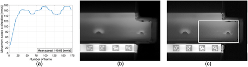
As the presented method is aimed towards a mobile application, it is of high interest to investigate whether µ-bolometer cameras could be used for the inspection. Uncooled µ-bolometer cameras are better suited in a mobile setup than quantum detector cameras with a Stirling motor as cooling device, since no moving parts are built in. However, the frame rate of such camera is much slower, usually 50 Hz. Furthermore, the thermal time constant of a µ-bolometer camera is significantly longer than the integration time of a quantum detector camera, which can lead to blurring of moving objects in image sequences. The previous measurement on the rail piece was repeated with similar speed, but instead of the cooled quantum detector camera the uncooled µbolometer camera was used to record the measurement with a frame rate of 50 Hz [11]. The spatial resolution for measurements with this camera was 0.29 mm/px. As the frame rate is lower than in the previous measurements, pixel shifts were calculated for all consecutive images, and not only in a given distance, as it has been done for the high frame rate records. The resulting speed profile can be seen in Figure 13a. Image registration with AprilTags also works for this recorded sequence, however the recorded images are blurred, as the object moves a couple of pixels during the thermal time constant of the camera (see Figure 13b). This means that in order to evaluate the scanning sequences further, each frame has to be deblurred before the sequence reordering is performed. In Ref [15] a method for deblurring infrared images is described. It is shown how parameters of the point spread function (PSF) can be calculated for a known motion speed in one direction. Image deconvolution is then used to reconstruct images and a Wiener filter reduces the noise. In the case of the recorded sequence the actual speed is known due to prior image registration and, therefore, a non-blind deconvolution can be used. As suggested in Ref [15], a k-factor of k = 0.005 is used for the Wiener filter to keep a higher contrast in the restored images, while also reducing the noise significantly (see Figure 13c).

Figure 13. a.) Calculated speed for a manual measurement and a camera frame rate of 50 Hz; b.) Frame 86 of the originally recorded sequence; c.) Deblurred image of frame 86 including ROI for evaluation.

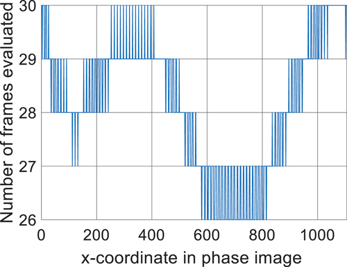
With all images deblurred, the quasi-stationary image sequence can be calculated as previously shown. This new sequence has 1103 px in x-direction. Figure 14 shows how many frames are evaluated in each column of this sequence. It can be seen that with increased speed the evaluated frames drop to 26, which means that only 26 temperature points are evaluated to the phase image for these columns.

Figure 14. Number of frames evaluated in each column of the quasi-stationary sequence.

For the phase image in Figure 15 the same method for adjusting phase values in each column is applied as previously described in Section 4.2. Figure 15 shows that all columns of the quasi-stationary image sequence were transformed correctly to phase image. Larger cracks and the two squats can be detected in this measurement; however, the signal contrast is too low to detect smaller cracks.

Figure 15. Phase image of the rail head measured with µ-bolometer camera and with a frame rate of 50 Hz.

The FLIR A615 µ-bolometer camera allows increasing its frame rate to 100 Hz by reducing the number of pixels to 640 × 240. Figure 16 shows the resulting phase image of a measurement, performed with a mean speed of 124 mm/s. The evaluation also included motion deblurring and rescaling of phase values. To compare the phase images of Figures 12, Figures 15 and 16 a homogeneous region in the lower central portion of the image was used to compute the mean value of the sound surface as well as the standard deviation (noise) in that area (see red area in Figure 16). A larger crack, which can be seen in all three evaluations, was chosen to compare the signal response of this crack (see green area in Figure 16). The signal response is calculated as the maximum phase value at the crack location minus the mean value of the sound surface. In Table 2 the signal responses as well as the signal-to-noise ratio (SNR) for all three phase images are compared.

Figure 16. Phase image of the rail head measured with µ-bolometer camera and with a frame rate of 100 Hz.

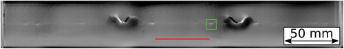
Table 2. Comparison of signal responses in three different phase images.

Phase image	Camera	Frame rate [Hz]	Mean speed [mm/s]	Mean value [°]	Noise [°]	Signal [°]	SNR [-]
Figure 12	IRCam VELOX 1310k SM	595	183	180.2	0.9	22.1	25.4
Figure 15	FLIR A615	50	150	178.0	3.6	21.6	6.1
Figure 16	FLIR A615	100	124	179.4	1.6	23.4	14.7

4.4. Estimation of evaluated frames and scanning speed

As it is shown in Figure 14, the presented method uses a certain amount of temperature data for each pixel column to calculate the phase value. Equation (1)(1) $n_{\mathit{phase}}=\frac{{\mathit{x}}_{\mathit{mov}}\cdot r_{\mathit{cam}}}{v_{\mathit{mean}}}\cdot f_{\mathit{cam}}$(1) shows how the number of frames which are evaluated in a specified segment can be estimated. At first, x_mov [px] the number of pixels in the moving direction, which are used for evaluation, is multiplied with the spatial resolution of the camera r_cam [mm/px]. This computes the length of the ROI in millimetre. Dividing this evaluation length with the mean scanning speed v_mean [mm/s] results in the time how long the camera records data for this pixel, as it is passing through the ROI. Multiplied this time duration by the camera’s frame rate f_cam [Hz] results in n_phase, the number of images recorded for this pixel, which are then used for the phase calculation:

(1) $n_{\mathit{phase}}=\frac{{\mathit{x}}_{\mathit{mov}}\cdot r_{\mathit{cam}}}{v_{\mathit{mean}}}\cdot f_{\mathit{cam}}$(1)

On the other hand, this equation can also be used to estimate the maximum speed, assuming a certain minimum number of images, required for the phase calculation. E.g. if at least 25 frames must be considered for the phase evaluation, this results in a maximum scanning speed of 190 mm/s for the measurement performed with a frame rate of 50 Hz with the current setup. Furthermore, this means a heating duration of about 0.19 s. By increasing the cameras frame rate the maximum scanning speed also can be increased. However, the original sequence will get blurrier and the referencing frames with AprilTags become too blurry, and this can lead to wrong image shift calculations. In Ref [16] it is shown that by using a quantum detector camera with 50 Hz it is possible to get good results even with a mean scanning speed of 230 mm/s.

5. Summary and discussion

In this work AprilTags were used to calculate the pixel shifts during scanning inductive pulse phase thermography with changing scanning speed. A metallic ruler was first spray-painted and AprilTags were engraved by removing paint with an industrial laser. This results in a referencing object with good visibility in the mid- and long-wave infrared spectrum. Scanning measurements are performed by moving the specimen and the referencing object through the field of a stationary inductor and recording the temperature change with a stationary infrared camera. The AprilTags recorded in each frame of the sequence are then used to register shifting between the frames. This information is used in the next step to eliminate the motion in the recorded images and to create a new quasi-static image sequence.

The registration algorithm performs very well in combination with the used AprilTags. High contrast between metallic tag and painted ruler allows generating a good contour image of each AprilTag. Since each Tag has a unique design, calculating the shifts via phase correlation works excellently. The used method also works on slightly blurred AprilTags, when using a µ-bolometer camera. In future work it is planned to recognise each AprilTag to obtain its identification number. This further will allow the localisation of the defects in the real world, since the pixel location of specific points in the evaluation result can be transferred to specific points on the specimen.

The quasi-static image sequence is used to calculate a pixel-wise Fourier transform to phase image. Pixels, which do not carry actual information, are excluded from the phase calculation. In the resulting phase images subsurface defects as well as surface defects can be excellently detected and localised, since phase images include the temporal change of the temperature. Single temperature images are affected by inhomogeneous heating and by inhomogeneous surface properties as emissivity, which makes it difficult to distinguish between artefacts and real defects. But using the proposed method and evaluating the phase images, these difficulties become negligible. Due to the changing scanning speed the number of temperature data used for Fourier transform varies from pixel to pixel, which may affect the defect depth estimation.

In many practical applications it is not possible to ensure a constant scanning speed, as it is the case for manual inspection. The proposed method allows a registration of the motion in an infrared image sequence itself, using a visual fiducial placed besides the measured object for registration. Therefore, no additional sensor is needed to measure the scanning speed. The successful measurements with a µ-bolometer camera show that such an application can also be achieved with cheaper camera systems, which are more suitable for a mobile setup. According to our experience, the registration using the AprilTags has even a higher accuracy than it could be achieved by a speed measurement sensor.

Acknowledgments

The authors gratefully acknowledge the financial support under the scope of the COMET program within the K2 Center “Integrated Computational Material, Process and Product Engineering (IC-MPPE)” (Project No 886385). This program is supported by the Austrian Federal Ministries for Climate Action, Environment, Energy, Mobility, Innovation and Technology (BMK) and for Labour and Economy (BMAW), represented by the Austrian Research Promotion Agency (FFG), and the federal states of Styria, Upper Austria and Tyrol.

Disclosure statement

No potential conflict of interest was reported by the author(s).

Additional information

Funding

The work was supported by the Österreichische Forschungsförderungsgesellschaft.

Notes on contributors

C. Tuschl

Christoph Tuschl received his MS in mechanical engineering. He started his PhD in 2022. His field of research is active thermography with a special focus on scanning pulse phase thermography. He has been working in the field of active thermography at the Chair of Automation, University of Leoben since 2014.

B. Oswald-Tranta

Beate Oswald-Tranta received her MS in electrical engineering. She made her PhD at the area of solid state physics, modelling and measuring of semiconductor structures for infrared detection. Since 2003 she works at the Chair for Automation, University of Leoben. Her research fields are automated non-destructive testing, thermography and image processing.

T. Agathocleous

Timotheos Agathocleous is currently pursuing his BS in mechanical engineering and working in the field of active thermography at the Chair of Automation, University of Leoben.

S. Eck

Sven Eck holds a PhD in experimental physics since 2003. From 2003 to 2009 he was an assistant professor at the University of Leoben at the Chair for Simulation and Modelling of Metallurgical Processes (SMMP). Since 2009 he is project manager of research projects at the Materials Center Leoben Forschung GmbH (MCL) with a focus on material development and material based condition monitoring for railway components; since 2015 he is also assistant to the general management of MCL.

References

- Oswald-Tranta B. Induction thermography for surface crack detection and depth determination. Appl Sci. 2018;8(2):257.
- Maldague X. Infrared and thermal testing. In: editor, Moore PO. Nondestructive testing handbook. 3rd ed. Columbus, OH: American Society for Nondestructive Testing; 2001. 718. 978-1-57117-044-6.
- Netzelmann U, Walle G, Lugin S, et al. Induction thermography: principle, applications and first steps towards standardization. Proceedings of the Quantitative InfraRed Thermography Conference Asia; Mamallapuram (India): 2015.
- Vrana J, Goldammer M, Baumann J, et al. Mechanisms and models for crack detection with inductions thermography. In Proceedings of the AIP Conference; Golden (Colorado): AIP; 2008. Vol. 975, p. 475–482.
- Srajbr C Induction excited thermography in industrial applications. In Proceedings of the 19th World Conference on Non-Destructive Testing; Munich, Germany; June 2016. p. 13–17.
- DIN 54183: 2018-02. Non-destructive testing - thermographic testing - Eddy-current excited thermography. [cited 2018 Jan 31]. Available from: https://www.din.de
- Oswald-Tranta B. Time-resolved evaluation of inductive pulse heating measurements. Quant Infrared Thermogr J. 2009;6(1):3–19.
- Oswald-Tranta B, Sorger M. Scanning pulse phase thermography with line heating. Quant Infrared Thermogr J. 2012;9(2):103–122.
- Olson E AprilTag: a robust and flexible visual fiducial system. In Proceedings of the 2011 IEEE International Conference on Robotics and Automation; May 2011; Shanghai, China: IEEE. p. 3400–3407.
- IRCAM Velox 1310k SM Datasheet. [cited 2022 June 9]. Available from: https://www.ircam.de/wp-content/uploads/2021/02/IRCAM_VELOX1310kSM_10%C2%B5m_Datasheet.pdf
- FLIR A615 25° datasheet. [cited 2022 June 9]. Available from: http://support.flir.com/DsDownload/Assets/55001-0102-en-US_A4.pdf
- Stock R, Kubin W, Daves W, et al. Advanced maintenance strategies for improved squat mitigation. Wear. 2019;436–437:203034.
- Tuschl C, Oswald-Tranta B, Eck S. Inductive thermography as non-destructive testing for railway rails. Appl Sci. 2021;11(3):1003.
- Tuschl C, Oswald-Tranta B, Eck S. Scanning inductive thermographic surface defect inspection of long flat or curved work-pieces using rectification targets. Appl Sci. 2022;12(12):5851.
- Oswald-Tranta B. Temperature reconstruction of infrared images with motion deblurring. J Sens Sens Syst. 2018;7(1):13–20.
- Tuschl C, Oswald-Tranta B, Agathocleous T, et al. Scanning pulse phase thermography with changing scanning speed. In Proceedings of the Quantitative InfraRed Thermografie Conference; Paris, France; 2022. p. 422–430.