A study of lactation curves in dairy cattle using the optimal design of experiments methodology

Abstract

In this paper, we have worked with some of the most popular models to fit the lactation curve. Lactation curves have received considerable attention in modelling dairy cattle milk production. These curves express the evolution over time of a cattle head’s milk yield. Observations of milk production over a cycle have usually been carried out periodically (i.e. daily, weekly or monthly). Optimal experiment design allows one to know the times when a herd’s milk production must be recorded. An experiment design is optimal when it achieves the best parameter estimates for the curve model. This work aims to study optimal designs for certain models such as quadratic polynomial, hyperbolic, exponentials and Wilmink models (WMs). Designs are observed to depend on models and must be compared to get to know if a design for a specific model has a good behaviour with another model. Design efficiency is the tool used for this comparison. Efficiency is a value between 0 and 1 – a design is good if its efficiency is close to 1. The WM designs perform well and are an improvement on those designs that are routinely used in daily observations.

Highlights

• Optimal experiment design allows one to know the times when a herd‘s milk production must be recorded.

• The use of optimal design methodology greatly reduces the number of instances when dairy production has to be recorded.

• Optimal designs reduce the costs of experimentation by allowing parameters to be estimated with fewer experimental runs.

Keywords:

• Lactation curves
• regression models
• optimal designs

Introduction

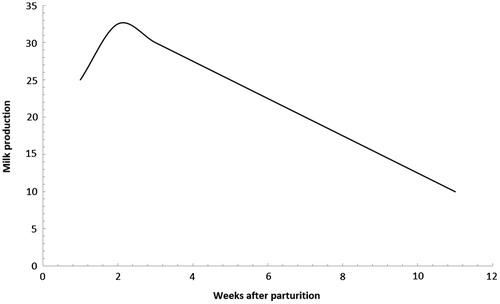
A lactation curve represents the evolution over time of a herd’s milk production during a specific lactation cycle. This cycle is the period from lactation onset after calving until the cow’s milk dries up. Lactation curves generally reach their peak yield after calving and then decrease steadily from then until drying up (Figure 1).

Figure 1. Standard shape of the lactation curve for dairy cattle. The plot shows the milk production as function of the weeks after the parturation.

Lactation curves allow the evaluation of important milk production characteristics such as maximum production and times to maximum production (Gipson and Grossman, 1990) or persistency (Gengler, 1996). These curves can help in herd management, particularly in assessing cattle heads’ nutritional and health status (Dudouet, 1982). These curves are also useful in predicting a cattle head’s total milk yield when only early lactation cycle observations are known.

Multiple statistical models have been used to describe lactation curves. Quintero et al. (2007), Cankaya et al. (2011), Macciotta et al. (2011), Graesbøll et al. (2016), Hossein-Zadeh (2016) and Melzer et al. (2017) reported on different lactation curve models, which are compared for dairy cattle. These papers show some models that can generally be expressed as $Y=\eta \left(t,\beta \right),$ where $Y$ stands for milk yield at week or day $t$ of lactation, and time $t$ is on a time interval $T$. Here $\beta$ is a vector which contains the unknown model parameters to be estimated from data. Function $\eta (t,\beta )$ can be either linear or nonlinear on $\beta$. Some of the models used to fit lactation curve data are: linear (LM) ${Y=\beta }_0+{\beta }_{1}t$, quadratic (QM) ${Y=\beta }_0+{\beta }_{1}t+{\beta }_2{t}^2$, hyperbolic (HM) ${Y=\beta }_0+{\beta }_{1}t+{\beta }_2{t}^{-1}$, inverse quadratic (IM) ${Y=t\left({\beta }_0+{\beta }_{1}t+{\beta }_2{t}^2\right)}^{-1}$, exponential (EM) ${Y=\beta }_1{e}^{-{\beta }_{2}t}$ or exponential with constant term (EMC) ${Y=\beta }_0+{\beta }_1{e}^{-{\beta }_{2}t}$.

This paper is focussed on the Wilmink model (WM), which is one of the most popular models used for lactation curve description. It is expressed as $Y={\beta }_0+{\beta }_{1}t+{\beta }_2{e}^{-kt},$ where parameter ${\beta }_0$ is associated with the level of production, ${\beta }_1$ with the production decrease after peak yield, ${\beta }_2$ with the production increase prior to peak yield, and $k$ is a parameter associated with the time of peak yield. Cankaya et al. (2011) characterised peak yield and the maximum production time. In Wilmink (1987) and many subsequent papers, parameter $k$ is fixed at $0.05$. Nevertheless, Torshizi et al. (2011) used values of $0.05$, $0.065,\mathrm{ }0.1$, and $0.61$ for $k$. The WM has three parameters when $k$ is fixed. Olori et al. (1999) concluded that the WM is the best three-parameter model for predicting mean herd yield. If $k$ is an unknown parameter, the WM has four parameters, $k$ being a nonlinear parameter and is called the Wilmink extended model (WEM).

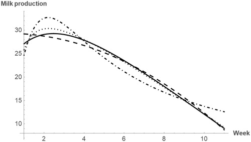
Some papers dealing with lactation models researched the use of several models to estimate the data and compared them using the coefficient of determination. Different conclusions were drawn regarding the best model for lactation period modelling. Figure 2 shows the plot of some of these functions.

Figure 2. Plot for some lactation models: QM (dashed line), HM (dotted line), IM (dot-dashed line) and WEM (solid line).

The WM is a modification of the Cobby–Le Du model (see Cobby and Le Du, 1978). This model includes particularity that post-peak milk yield is modelled as a linear decline function and combines exponential and linear models. Both models are related to a model proposed by Wood (1967), which is expressed as $Y={\beta }_0{t}^{{\beta }_1}{e}^{-{\beta }_{2}t}$. The Wood model is widely used for lactation curve descriptions in dairy cattle and lactation predictions in cows and goats. Nonetheless, the results from the Wood model are improved by the WM.

To estimate these models’ parameters, the researcher requires certain observations; namely, a sample of $t$ and $Y\mathrm{ }$values. The optimal design of experiments methodology can be applied because it aims to find the best $t$ values where variable $Y$ is to be observed (i.e. the days or weeks when milk production must be registered). In general, model estimation includes several steps in which the researcher can control the independent variable $t$. Firstly, given a theoretical model, one attempts to find ‘optimum’ values for the design variable, $t$, in the range of experimental interest, $T$. This search is carried out with respect to an optimality criterion which is chosen according to the final analysis goal – parameter estimation or hypothesis testing. Secondly, variable $Y\mathrm{ }$is observed in the optimum $t$ allocations given by the optimum design. Finally, the model is estimated using these observations.

Optimal designs have been applied to a wide range of fields such as biomedicine (Campos-Barreiro and López-Fidalgo, 2013), pharmacokinetics and pharmacodynamics (Kitsos and Kolovos, 2013), and agricultural studies (Martínez-López et al., 2009).

This paper researches optimal experimental designs for lactation curves. However, these designs depend on the particular model and the optimality criterion. Therefore, several lactation models are considered in the paper. With the objective of estimating the model parameters, a commonly adopted criterion is D-optimality, which obtains D-optimal designs. By using such designs, the best estimates for a model’s unknown coefficients (parameters) are achieved.

Material and methods

The statistical regression model is expressed as: $Y=\eta \left(t,\beta \right)+ϵ,\mathrm{ }t\in T,$ where $Y$ is the response variable, $t$ is the independent variable, and $\beta$ is a vector of $p$ unknown parameters that we have to estimate from the observations. The $ϵ$ term stands for the random errors with zero mean and constant variance.

Some definitions of optimal experimental design theory

An experimental design $\xi$ is a collection of $t$ values where $Y$ is to be observed. The design is made-up of $n$ different support points $t_1$, $t_2$, $\dots$, $t_n$, and their respective weights $w_1$, $w_2$, $\dots$, $w_n$ (relative frequencies, $w_1+w_2+\dots +w_n=1$). A weight, $w_i$, is the proportion of the total observations taken at time $t_i$, and this can be considered as a probability measure (Kiefer, 1974). If we want $N$ observations to estimate the model, then we round up the ${Nw}_i$ values to know the number of observations at points $t_i$.

An optimal design, ${\xi }^{\mathrm{*}}$, includes the best points and weights with respect to an optimality criterion. Of the different criteria in the literature, we are going to consider the D-optimality criterion because it relates to the estimation quality of the model parameters.

The advantage of using optimal designs is that we control the times when the observations are taken, leading to the best possible parameter estimation. The accuracy of an estimator is measured by its variance, and this is part of a matrix known as the information matrix. This matrix is the main tool when looking for optimal designs.

When the function $\eta \left(t,\mathrm{ }\beta \right)$ is differentiable with a continuous derivative for every parameter, ${\beta }_i$, with $\nabla \eta (t,\mathrm{ }\beta )\mathrm{ }$as its gradient vector, the information matrix is defined by $M\left(\xi ,\mathrm{ }\beta \right)={\sum }_{i=1}^n{w}_i\nabla \eta (t_i,\mathrm{ }\beta )\nabla {\eta (t_i,\mathrm{ }\beta )}^T.$ The inverse of the information matrix is asymptotically proportional to the covariance matrix of the parameter estimators. For this reason, many optimality criteria are formulated in terms of this matrix; for example, the D-optimality criterion is related to the determinant of the information matrix. A D-optimal design maximises this determinant, which is equivalent to minimising that of the covariance matrix, so D-optimal designs minimise the volume of the confidence region of the regression parameter vector, $\beta$.

The General Equivalence Theorem is a useful tool to check whether a design is optimal. This theorem states that a design ${\xi }^{\mathrm{*}}$ is D-optimal if and only if $d\left(t,{\xi }^{\mathrm{*}},\beta \right)={\nabla \eta \left(t,\beta \right)}^T{M}^{-1}\left({\xi }^{\mathrm{*}},\beta \right)\nabla \eta \left(t,\beta \right)\le \mathrm{ }p,\mathrm{ }$for all values of $t$ in $T$, with $p$ being the number of model parameters. Furthermore, the maxima of $d(t,\mathrm{ }{\xi }^{\mathrm{*}},\mathrm{ }\beta )$ occur at the ${\xi }^{\mathrm{*}}$ support points. Function $d(t,\mathrm{ }{\xi }^{\mathrm{*}},\mathrm{ }\beta )$ is called the variance function.

For non-linear models, the variance function and the information matrix depend on unknown parameters. The simplest way to deal with this problem is by using a single prior guess for the unknown parameters, obtaining locally optimal designs. Such knowledge is often available from preliminary studies. Optimal designs will depend on this initial information.

Results

The results of this study are the optimal experimental designs for the Wilmink lactation curves. These designs contain the times when observations must to be recorded. The D-optimality criterion is used. The optimal designs are presented in several tables.

We will consider the general design space $T=[a,\mathrm{ }b]$, $0<a<b<+\mathrm{\infty }$, and two cases depending on parameter $k$. If $k$ is a known value, we employ the usual WM, which has three parameters $\beta ={\left({\beta }_0,{\beta }_1,{\beta }_2\right)}^{\mathrm{T}}$. If $k$ is an unknown parameter, we employ the WEM, which has four parameters $\beta ={\left({\beta }_0,{\beta }_1,{\beta }_2,k\right)}^{\mathrm{T}}$. Consequently, the optimal designs differ in each case.

Wilmink model

The D-optimal design, ${\xi }^{\mathrm{*}}$, for WM in the interval $T=[a,\mathrm{ }b]$, with $0<a<\mathrm{b}<+\mathrm{\infty }$, is supported at exactly three points: $t_1=a$, $t_2=-\frac{1}{k}\log \left(\frac{e^{-ka}-e^{-kb}}{k(b-a)}\right)$ and $t_3=b$. The respective weights are $w_1=w_2=w_3=1/3.$

For the proof of the above results, we have taken into account the gradient vector $\nabla \eta \left(t,\beta \right)={(1,t,e^{-kt})}^{\mathrm{T}}$ and the results in Karlin and Studden (1966). In this case the information matrix and the variance function do not depend on unknown parameters, so they can be denoted by $d(t,\xi )$ and $M(\xi )$, respectively. Studying the maxima and minima of $d(t,\mathrm{ }\xi )$, and applying the General Equivalence Theorem, we conclude that $t_1=a$, $t_3=b$ and $t_{2\mathrm{ }}$is an interior point in $[a,\mathrm{ }b]$, which is the solution of $\partial \left|M\right(\xi \left)\right|/\partial t_2=0$.

We can observe that interior support point $t_2\mathrm{ }$tends to the midpoint of the interval $(a+b)/2,$ when $k\to 0$ and $t_2$ tends to $a,$ when $k\to +\mathrm{\infty }$.

According to Wilmink (1987), the lactation cycle length was $305$ days, making $T=\left[\mathrm{1,305}\right]$. Consequently, the observations must to be recorded at days $t_1=1$, $t_2=-\frac{1}{k}\log \left(\frac{e^{-k}-e^{-305\mathrm{ }k}}{304\mathrm{ }k}\right)$ and $t_3=305$. For $k=0.05$, considered in Wilmink (1987), the optimal value of $t_2$ is $55.426$. Nevertheless, in the Wilmink work milk production was observed on each of the 305 days; that is, a uniform design with $305$ support points $t_1=1,\mathrm{ }{t}_2=2,\mathrm{ }\dots ,t_{305}=\mathrm{ }305$ was considered; this will be denoted by ${\xi }_{305}$.

We can compare designs ${\xi }_{305}$ and ${\xi }^{\mathrm{*}}$ through the determinant of the information matrix: $\left|M\right({\xi }_{305}\left)\right|=138.18$ and $\left|M\right({\xi }^{\mathrm{*}}\left)\right|=1766.25$; the second determinant being greater than the first because it corresponds to the D-optimal design. Applying the D-optimality criterion, design ${\xi }^{\mathrm{*}}$ is better than design ${\xi }_{305}$ because its determinant is greater as is the meaningful information. Therefore, the estimated parameters will be more precise if we use design ${\xi }^{\mathrm{*}}$.

A measurement of a given design’s behaviour, $\xi$, relative to the D-optimal design, ${\xi }^{\mathrm{*}}$, is the D-efficiency, which is calculated as: $${Eff}_{\mathrm{D}}\left(\xi \right)={\left(\frac{\left|M\right(\xi \left)\right|}{\left|M\right({\xi }^{\mathrm{*}}\left)\right|}\right)}^{1/p},$$ where $p$ is the number of unknown parameters. This value is within $\left[\mathrm{0,1}\right]$ and ${Eff}_{\mathrm{D}}\left(\xi \right)=0.5$ meaning that design $\xi$ needs to double the total number of observations to perform as well as optimal design ${\xi }^{\mathrm{*}}$. The D-efficiency of ${\xi }_{305}$ is only 0.43, which is a very low value.

Torshizi et al. (2011) considered other values for $k$; namely, $0.065$, $0.1$ and $0.61$. For these values, the D-optimal designs in$\mathrm{ }T=[1,\mathrm{ }305]$ are equally supported at three points – these are the ends of this interval and the points 46.9, 35.14, and 9.56, respectively.

Since D-optimal design depends on the value of $k$, we need to analyse whether the D-optimal design for a given $k$ value behaves well for another value. Table 1 reports the D-efficiencies of the optimal design for $k=k_2$ when it is used to estimate another model with a different value, $k=k_1$. For this, we considered the values of $k$ in Torshizi et al. (2011). For instance, the value $0.994$ in Table 1 implies that the D-optimal design for $k_2=0.065$ behaves very well in estimating the WM with $k_1=0.05$. However, the D-optimal design for $k=0.61$ does not behave well in estimating the model with $k_1=0.05$, because its D-efficiency is $0.544$. Table 1 also includes the efficiencies of daily design ${\xi }_{305}$. We can see that the efficiencies for the various D-optimal designs are higher than for the daily design used in Wilmink (1987).

TABLE 1. Efficiencies for WM D-optimal designs.

	WM D-optimal design
WM design	True values $k_1$
Miss values $k_2$	$0.050$	$0.065$	$0.100$	$0.610$
$0.050$	$1$	$0.995$	$0.970$	$0.897$
$0.065$	$0.994$	$1$	$0.988$	$0.917$
$0.100$	$0.956$	$0.984$	$1$	$0.945$
$0.610$	$0.544$	$0.629$	$0.743$	$1$
${\xi }_{305}$	$0.428$	$0.397$	$0.350$	$0.221$

Efficiency is the behaviour of D-optimal designs for Wilmink models (WM) with $k_2$ when used to estimate WM with true value $k_1$.

Wilmink extended model

Here, we consider that $k$ is another unknown parameter. The WEM is nonlinear with four parameters $\beta ={({\beta }_0,\mathrm{ }{\beta }_1,\mathrm{ }{\beta }_2,\mathrm{ }k)}^{\mathrm{T}}$ . The information matrix depends on parameter $k$ and is denoted by $M\left(\xi ,\mathrm{ }k\right)$. Locally D-optimal designs will be obtained because there is a need for prior information regarding $k$; for example, from previous experiments, this will be denoted by $k_0$.

The locally D-optimal design ${\xi }^{\mathrm{*}}$ for WEM in $T=[a,b]$, $0<\mathrm{ }a<b\mathrm{ }<+\mathrm{\infty }$, and $k=k_0$ is equally supported at exactly four points. Two of the support points are the boundary points of the interval ($t_1=\mathrm{ }a$ and $t_4=\mathrm{ }b$). For the other points, $t_2$ and $t_3$, we do not have an explicit expression but they are the solutions to the equations of $\partial \left|M\left(\xi ,\mathrm{ }{k}_0\right)\right|/\partial t_2=\mathrm{ }0$ and $\partial \left|M\left(\xi ,\mathrm{ }{k}_0\right)\right|/\partial t_3=0$. Table 2 reports the support points of locally D-optimal designs in $\left[\mathrm{1,305}\right]$ for WEM and the values of $k$ in Torshizi et al. (2011).

TABLE 2. Support points of WEM locally D-optimal designs in $[1,305]$.

$k$	$t_1$	$t_2$	$t_3$	$t_4$
$0.050$	$1$	$19.85$	$92.32$	$305$
$0.065$	$1$	$15.75$	$77.05$	$305$
$0.100$	$1$	$10.75$	$56.28$	$305$
$0.610$	$1$	$2.64$	$13.70$	$305$

D-optimal designs are equally supported at $t_1$, $t_2$, $t_3$, and $t_4$. WEM: Wilmink extended model.

Table 3 compares the behaviour of the different locally D-optimal designs in Table 2. Efficiencies for daily design ${\xi }_{305}$ are included. In this case, efficiencies are strongly influenced by parameter $k$. Significantly lower efficiency is obtained when $k_2$ differs from the true $k_1$ value. As in WM, the daily design efficiencies are very small.

TABLE 3. Efficiencies for WEM D-optimal designs.

	WEM D-optimal design
WEM design	True value $k_1$
Miss value $k_2$	$0.050$	$0.065$	$0.100$	$0.610$
$0.050$	$1$	$0.975$	$0.834$	$0.015$
$0.065$	$0.976$	$1$	$0.934$	$0.049$
$0.100$	$0.851$	$0.938$	$1$	$0.190$
$0.610$	$0.184$	$0.245$	$0.384$	$1$
${\xi }_{305}$	$0.333$	$0.291$	$0.221$	$0.092$

Efficiency is the behaviour of the D-optimal designs for WEM with $k_2$ when used to estimate WEM with true value $k_1$. WEM: Wilmink extended model.

In Table 4, we include the efficiencies of the locally D-optimal designs for WEM when they are used to estimate the WM. We can use a four-point optimal design for WEM to estimate a three-parameter WM but it is not possible to use an optimal design for a WM (three points) to estimate a WEM (four parameters).

TABLE 4. Efficiencies of locally D-optimal designs for WEM with respect to those for WM, for different $k$ values.

	WM D-optimal design
WEM design	Value $k$
Value $k$	$0.050$	$0.065$	$0.100$	$0.610$
$0.050$	$0.860$	$0.861$	$0.874$	$0.864$
$0.065$	$0.865$	$0.861$	$0.868$	$0.880$
$0.100$	$0.871$	$0.867$	$0.863$	$0.902$
$0.610$	$0.616$	$0.673$	$0.762$	$0.865$

WEM: Wilmink extended model; WM: Wilmink model.

Discussion

A variety of different mathematical models have been used to research the lactation curve shape. Working with these models, a particular problem is collecting data to estimate the parameters as precisely as possible. To do this, it is necessary to design the experiment. There is relevant literature regarding D-optimal designs for regression models. We then set the results for those models applied to lactation – namely, the polynomial, hyperbolic, inverse quadratic and exponential models. Firstly, we offer the theoretical insight and, after that, the numerical results will be included in Table 5. Depending on the model, we will have to record the observations at different times, so we compare the behaviour of a model-specific D-optimal design when used to estimate another model. Finally, a web application is presented to obtain the optimal designs for this research.

TABLE 5. Support points for D-optimal designs for some lactation models.

Model	Support points
LM	$1$			14
EM^(1)	$1$			$14$
HM	$1$	$3.74$		$14$
IM^(2)	1	$3.41$		$14$
WDM^(3)	$1$	$4.56$		$14$
EMC^(1)	$1$	$7.04$		$14$
QM	$1$	$7.50$		$14$
WM	$1$	$7.15$		$14$
WEM^(4)	$1$	$4.32$	$10.12$	$14$

Lactation models namely, linear (LM), exponential (EM), hyperbolic (HM), inverse quadratic (IM), Wood (WDM), exponential with constant term (EMC), quadratic (QM), Wilmink (WM), and Wilmink extended (WEM), in $[1,14]$. With best guesses from Landete-Castillejos and Gallego (2000): ⁽¹⁾${\beta }_2^0=0.03307$; ⁽²⁾${\beta }_0^0=0.0002865$; ${\beta }_1^0=0.0002117$; ${\beta }_2^0=0.0000301$; ⁽³⁾${\beta }_1^0=0.33269$; ${\beta }_2^0=0.09319;$ and ⁽⁴⁾$k_0=0.05$.

Polynomial model

According to Karlin and Studden (1966), the D-optimal design for the polynomial model of degree $r$, on interval $[-1,\mathrm{ }1]$, is equally supported at $r+1$ points, which are the roots of the polynomial $(1-t^2){L\mathrm{\text{'}}}_r\left(t\right)$, where ${L\mathrm{\text{'}}}_r\left(t\right)$ is the derivative of the Legendre polynomial of degree $r$. If $z_i$ are the support points in $[-1,\mathrm{ }1]$, then $t_i=\left(1+\mathrm{ }b+(b-1)z_i\right)/2$ are the support points on interval $[1,b]$. Both ends of the design space are always support points.

Hyperbolic model

The D-optimal design in $[a,b]$, with $0<a<b$, is equally supported at $t_1=a$, $t_2=\sqrt{ab}$ and $t_3=b$. In particular, the D-optimal design is equally supported at $\left\{1,\sqrt{b},b\right\}$ for the interval $[1,b]$.

Inverse quadratic polynomial model

From Haines (1992), the locally D-optimal design is equally supported at $t_1=\tau /\rho$, $t_2=\tau$ and $t_3=\tau \rho$, with $\tau =\sqrt{{\beta }_0^0/{\beta }_2^0}$, $\rho =\left(\delta +\sqrt{{\delta }^2-4}\right)/2$, $\delta =\left(\gamma +1+\sqrt{{\gamma }^2+6\gamma +33}\right)/2$ and $\gamma ={\beta }_1^0/\sqrt{{\beta }_0^0{\beta }_2^0}$, for initial values$\mathrm{ }{\beta }_0=\mathrm{ }{\beta }_0^0$, ${\beta }_1={\beta }_1^0$ and ${\beta }_2={\beta }_2^0$. If $t_1$ or $t_3$ are not included in the design interval, the support point is then fixed at the end of the interval and the other support points are calculated as shown in Haines (1992).

Exponential model

Han and Chaloner (2003) obtained the locally D-optimal design in interval $[1,b]$ is equally supported at two points: $t_1=1$ and $t_2=\text{min}\left\{1+\frac{1}{{\beta }_2^0},b\right\}$, for ${\beta }_2={\beta }_2^0$.

Exponential model with constant term

Han and Chaloner (2003) also calculated the locally D-optimal design for the exponential model with a constant term in $[1,b]$. For ${\beta }_2={\beta }_2^0$ it is equally supported at three points $t_1=1$, $t_2=\frac{e^{{\beta }_2^0}\left(1+{\beta }_2^{0}b\right)-e^{{\beta }_2^{0}b}\left(1+{\beta }_2^0\right)}{{\beta }_2^0\left(e^{{\beta }_2^0}-e^{{\beta }_2^{0}b}\right)}$ and $t_3=b$.

Table 5 reports the optimal designs for the above models in the interval $T=\left[\mathrm{1,14}\right]$ considered by Landete-Castillejos and Gallego (2000). This design space corresponds to monthly observations of lactation yield throughout a cycle. All designs in Table 5 are equally supported. Some of the designs are locally optimal designs so they are obtained for initial parameter values found in Landete-Castillejos and Gallego (2000). For example, EM⁽¹⁾ is the locally D-optimal design for the exponential model with ${\beta }_2^0=0.03307$. IM⁽²⁾ is the locally D-optimal design for the inverse quadratic polynomial model with ${\beta }_0^0=0.0002865$, ${\beta }_1^0=0.0002117$ and ${\beta }_2^0=0.0000301$. Table 5 also includes the locally D-optimal design for WEM with $k=0.05$ and the locally D-optimal design for the Wood model (WDM) with ${\beta }_1^0=0.33269$ and ${\beta }_2^0=0.09319$.

Table 6 summarises the performances of the optimal designs in Table 5 in terms of their efficiencies. We must emphasise the good performance of some of these designs for different lactation curves, with efficiencies close to $1$, and the low efficiency always shown by the monthly design ${\xi }_{14}$.

TABLE 6. Efficiency study for optimal design for lactation models.

		D-optimal design for lactation models
	LM	EM	HM	IM	WDM	EMC	QM	WM
LM	$1$	$1$
EM	$1$	$1$
HM	$0.861$	$0.845$	$1$	$0.994$	$0.980$	$0.803$	$0.762$	$0.794$
IM	$0.869$	$0.853$	$0.997$	$1$	$0.958$	$0.756$	$0.714$	$0.747$
WDM	$0.844$	$0.832$	$0.987$	$0.967$	$1$	$0.894$	$0.859$	$0.886$
EMC	$0.817$	$0.826$	$0.858$	$0.702$	$0.889$	$1$	$0.997$	$1$
QM	$0.817$	$0.829$	$0.825$	$0.653$	$0.851$	$0.997$	$1$	$0.998$
WM	$0.817$	$0.827$	$0.850$	$0.690$	$0.879$	$1$	$0.998$	$1$
WEM	$0.775$	$0.864$	$0.864$	$0.876$	$0.898$	$0.865$	$0.866$	$0.865$
${\xi }_{14}$	$0.620$	$0.629$	$0.676$	$0.676$	$0.681$	$0.671$	$0.671$	$0.671$

LM: linear; EM: exponential; HM: hyperbolic; IM: inverse quadratic; WDM: Wood; EMC: exponential with constant term; QM: quadratic; WM: Wilmink; WEM: Wilmink extended; ${\xi }_{14}$: monthly design on space $[1,14]$.

We have created a Web application with the R Shiny software. This application allows one to obtain the optimal design for any of the models discussed, and for an interval $T=[1,b]$. We can estimate and draw the models for our experimental data. The Web application is available at https://imor.shinyapps.io/lactancy/

Conclusions

Milk yield over the course of the lactation cycle follows a curvilinear pattern, so a suitable function is required to model this curve. Eight functions (namely: linear, exponential, hyperbolic, inverse quadratic, exponential with constant term, quadratic, Wilmink and Wilmink extended) are investigated to model the lactation curve. The optimal designs for these models are studied in this paper.

The use of optimal design methodology greatly reduces the number of instances when dairy production has to be recorded. Consequently, milk production does not have to be observed every day or weekly. To obtain the best parameter estimates, one only has to study the days proposed by the optimal design. Optimal designs reduce the costs of experimentation by allowing parameters to be estimated with fewer experimental runs.

Efficiency was used to compare optimal design performance. This method allows one to compare models under different conditions. Table 5 shows two groups within the 3-support-point D-optimal designs. The hyperbolic, the inverse quadratic polynomial and the Wood models show a similar behaviour and high efficiency. Another group includes the exponential model with constant term, the quadratic polynomial model, and the WM, which likewise share similar characteristics.

The results of this work support the idea that the WM provides good performance. Its efficiencies are high for the cases considered. It greatly improves the design with routinely used with daily observations. The main disadvantage of the WM is the importance of having an accurate parameter value for the exponent. Inappropriate specifications for this parameter can lead to low efficiencies.

Funding

This study was financially supported by Grant MTM2013-479879-C2-1-P Spanish Ministerio de Economía y Competitividad.

Disclosure statement

No potential conflict of interest was reported by the authors.

References

- Campos-Barreiro S, López-Fidalgo J. 2013. Experimental designs for a Benign Paroxysmal Positional Vertigo model. Theor Biol Med Model. 10:1–14.
- Cankaya S, Unalan A, Soydan E. 2011. Selection of a mathematical model to describe the lactation curves of Jersey cattle. Archiv Fur Tierzucht. 54:27–35.
- Cobby JM, Le Du LP. 1978. Fitting curves to lactation data. Animal Prod. 26:127–134.
- Dudouet E. 1982. Courbe de lactation théorique de la chèvre et applications (Theoretical lactation curve of the goat and its applications). Point Vet. 14:53–61.
- Gengler N. 1996 Persistency of lactation yields: a review. Proceedings of the International Workshop on Genetic Improvement of Functional Traits in Cattle, Gembloux, Belgium. Interbull Bull. 12:87–96.
- Gipson TA, Grossman M. 1990. Lactation curves in dairy goats: a review. Small Ruminant Res. 3:383–396.
- Graesbøll K, Kirkeby C, Nielsen SS, Halasa T, Toft N, Christiansen LE. 2016. Models to estimate lactation curves of milk yield and somatic cell count in dairy cows at the herd level for the use in simulations and predictive models. Front Vet Sci. 3:115.
- Haines LM. 1992. Optimal design for inverse quadratic polynomials. South African Stat J. 26:25–41.
- Han C, Chaloner K. 2003. D- and c-optimal designs for exponential regression models used in pharmacokinetics and viral dynamics. J Stat Plan Inference. 115:585–601.
- Hossein-Zadeh NG. 2016. Modelling lactation curve for fat to protein ratio in Holstein cows. Animal Sci Papers Rep. 34:233–246.
- Karlin S, Studden WJ. 1966. Optimal experimental designs. Ann Math Stat. 37:783–815.
- Kiefer J. 1974. General equivalence theory for optimum designs. Approximate theory. Ann Stat. 2:849–879.
- Kitsos CP, Kolovos KG. 2013. A compilation of the D-optimal designs in chemical kinetics. Chem Eng Commun. 200:185–204.
- Landete-Castillejos T, Gallego L. 2000. Technical note: the ability of mathematical models to describe the shape of lactation curves. J Animal Sci. 78:3010–3013.
- Macciotta NPP, Dimauro C, Rassu SPG, Steri R, Pulina G. 2011. The mathematical description of lactation curves in dairy cattle. Ital J Animal Sci. 16:213–223.
- Martínez-López I, Ortiz-Rodríguez I, Rodríguez-Torreblanca C. 2009. Optimal designs for weighted rational models. Appl Math Lett. 22:1892–1895.
- Melzer N, Trißl S, Nürnberg G. 2017. Estimating lactation curves for highly inhomogeneous milk yield data of an F2 population (Charolais x German Holstein). J Dairy Sci. 100:9136–9142.
- Olori VE, Brotherstone S, Hill WG, McGuirk BJ. 1999. Fit of standard models of the lactation curve to weekly records of milk production of cows in a single herd. Livestock Prod Sci. 58:55–63.
- Quintero JC, Serna JI, Hurtado NA, Rosero Noguera R, Cerón-Muñoz MF. 2007. Modelos matemáticos para curvas de lactancia en ganado lechero. Rev Colom Cienc Pec. 20:149–156.
- Torshizi ME, Aslamenejad AA, Nassiri MR, Farhangfar H. 2011. Comparison and evaluation of mathematical lactation curve functions of Iranian primiparous Holsteins. South African J Animal Sci. 41:105–115.
- Wilmink J. 1987. Comparison of different methods of predicting 305-day milk yield means calculated from within herd lactation. Livestock Prod Sci. 17:1–17.
- Wood PDP. 1967. Algebraic model of the lactation curve in cattle. Nature. 216:164–165.