Bayes factors revealed selection signature for time to market body weight in chicken: a genome-wide association study using BayesCpi methodology

Abstract

Bayes Cπ methodology due to the simultaneous use of all SNPs in a random regression model is an alternative to overcome the overestimation of SNPs effects and excess of false positives. Hence, the present study was performed to identify causal single nucleotide polymorphisms (SNPs) associated with body weight (BW) and their pattern of significance over time from 2 to 8 weeks of age, in an F2 crossbred chicken population using Bayes Cπ methodology. Illumina 60 K SNP bead chip was used to genotype 312 F2 chicks. Sixteen SNPs distributed over 8 chromosomes had a Bayes Factor (BF) greater than 150 for BW in different ages. 14 different genes harbouring these SNPs (±250 kb), of which 12 were protein-encoding (DKK2, LEF1, RASGEF1C, FOXP1, LPCAT1, AKR1D1, GPR137C, EIF2AK3, ROR1, AKR1D1, LRFN5 and XPO7) and two were noncoding RNAs (LOC101751953 and LOC101751953). According to the obtained results, GGA1 and GGA4 were the most important chromosomes containing QTLs associated with observed traits. Different genetic regions were responsible for body weight in early and late ages. The various number of significant Bayes factors across different weeks of ages may indicate the artificial selection for market weight in a given age which has driven larger SNPs effects in intended weeks for desired market weight for the two groups.

Highlights

• My research outputs resulted in discovering associated genes and pathways related to gain growth and body weight in chicken. The identified genes in this study can be used in poultry breeding programs. Therefore, this leads to reduced feed costs and increase revenue.

Keywords:

• Body weight
• genome-wide association study
• Bayesian analysis
• chicken
• selection signature

Introduction

Body weight is a complex quantitative trait that is influenced by a large number of genes, each with different sizes and types (Goddard and Hayes 2009). As body weight is the most important trait in broilers especially for a specific stage of life, therefore identification of causative genetic loci for this trait can be essential to enhance genetic improvement by marker-assisted selection (Goddard and Hayes 2009).

The combination of natural and artificial selection for production traits over time in chicken can leave selection signatures in the genome (Walugembe et al. 2018; Weng et al. 2020). Artificial selection has been proved to influence significantly on the genomic loci associated with specific traits of an organism. Also, the relationship among the artificial selection, genomic regions, and interesting traits represented that recent artificial selection can increase runs of homozygosity at certain genetic markers and provide insight into the process of artificial selection (Kim et al. 2018)

The availability of dense marker genotypes for farm animals in recent years has made it possible to associate genetic markers such as single nucleotide polymorphisms (SNPs) with phenotypes of quantitative traits using genome-wide association study (GWAS). Generally, GWAS intends to detect significant SNPs to identify QTLs or causal genes for an interesting trait and alternatively enables to estimate the SNP-based heritability of the trait (Maher 2008). GWASs have firstly conducted based on the least-squares methodology (Costa et al. 2015), which has several drawbacks. Currently, GWA studies sufficiently improved by using variance component model (Kang et al. 2010) and mixed linear models controlling simultaneously the population structure and identical by descent issues between genotyped individuals for achievement of more accurate signals (Zhang et al. 2010 ).

First of all, SNPs enter the analysis individually so that it may exceed the false positive and overestimation of SNPs effects due to multiple testing (Peters et al. 2012). Choosing the right correction to avoid problems due to multiple testing is still a challenge (Wakefield 2009). An alternative to overcome these problems is to apply all SNPs simultaneously in a random regression model (Costa et al. 2015). Since the quantitative traits are influencing by a large number of SNPs, the model that analysis all markers simultaneously might be more accurate in comparison with models that analyzes markers individually (van den Berg et al. 2013).

Additionally, the F2 population designed for GWAS is more advantageous than a random population in reducing false positives and improving the accuracy of mapping (Ledur et al. 2010). Given that in most animal breeding studies the importance of statistical methods was considered and Bayesian methods based on Gibbs sampling techniques have been concerned. Although there is a published study on the present data using a generalised linear model (GLM) and compressed mixed linear model (cMLM) (Emrani et al. 2017), we hypothesised that there would be differences in the size and locations of important regions if using other statistical methods such as Bayesian methodologies. Alongside, SNP-based GWAS provides a useful framework with which to carry out genomic analyses. So, the goal of this study was conducted to test the above hypothesis to identify SNPs surrounding the genes associated with body weight traits through SNP-based GWAS using the Bayes Cpi method.

Material and methods

Phenotypic data

Phenotypic data used in this study was collected from an F2 generation descended from reciprocal crosses between a commercial broiler line named Arian (AA) and an Iranian indigenous chicken (NN) named Urmia. These birds are bred as a dual-purpose breed (eggs and meat production). Arian line chickens are a commercial fast-growing broiler strain and Urmia population is a slow-growing indigenous strain in Iran. Arian chickens have been under strong selection for body weight and meat quality traits. Otherwise, the Urmia chicken is an indigenous slow growth population under natural selection for natural conditions and more resistant to diseases and pathogens than Arian chickens. The probable genomic distance between these two led us to use the benefits of the F2 generation for association studies based on LD patterns by generating an F2 population through reciprocal crosses between Arian and Urmia chickens. Each of F1 males was crossed to 4–8 females and finally, 450 F2 birds produced in six different hatches, 52 full-sib and 8 half-sib families. Birds were housed individually in battery cages and body weight of all birds recorded weekly from 2 to 8 weeks of age. On day 8, birds were moved to individual cages with a temperature of 30 °C and gradually decreased to reach a final temperature of 22 °C. Chickens were fed starter diet (22.8% CP and 3025 kcal of ME/kg) for the first two weeks, a crumbled grower diet (20% CP and 2960 kcal of ME/kg) between 3 and 7 weeks; and a crumbled finisher diet (18% CP and 3070 kcal of ME/kg) on the week 8 of age. Chickens were not vaccinated against any diseases. Feed and water were provided ad libitum (Begli et al. 2017).

To increase the accuracy of measurements, 8 hours of fasting were applied to birds before each weighing.

Genotyping and quality control

A random collection of 312 birds were Genotyped using blood samples using Illumina 60 k SNP chip (Illumina Inc., San Diego, CA) (Begli et al. 2017). Each sample was genotyped for 54,340 SNP markers. Data quality controls performed by PLINK 1.9 software. SNPs with missing genotype greater than 10% and minor allele frequency (MAF) smaller than 5% as well as SNPs with p-value less than 1 × 10⁻⁶ in Hardy-Weinberg test was removed from the analysis (Begli et al. 2017). The total number of SNPs and population used for analysis in each age are shown in Table 1.

Table 1. Summary of the phenotypic and genotypic data used for the analysis in different weeks of ages.

Birds age (week)	Number of birds	Number of SNPs
2	294	43588
3	292	43569
4	305	43605
5	304	43588
6	299	43577
7	307	43622
8	301	43577

Statistical analysis

SNP effects estimated using the Bayes Cπ methodology. This method splits the SNPs into two categories. One category consists of the SNPs having effects and the other category for non-effective SNPs on the phenotypic trait (Habier et al. 2011). Starting values for genetic variance and the variance of residual were calculated by DMU software (Madsen and Jensen, 2002) and Gibbs sampling was conducted with Markov Chain Monte Carlo (MCMC) technique. The number of iterations to reach the convergence set to be 100,000 iterations. A number of 20,000 burn-in and a sampling interval of 100 used to calculate the average posterior probability of the parameters. To reach a stable posterior distribution in the Bayesian analysis, we start from a starting point which is called prior parameter which is not informative enough based on the data in MCMC chain. Therefore, there is some fluctuation at the beginning of the chain to estimate the posterior parameter and the posterior distribution. Usually, this fluctuation period discarded from final calculation of the parameters (genetic variance) which called burn-in phase. After this phase the fluctuation becomes more stable around a value that we call it convergence of the parameter. The convergence diagnostic of Markov chain posterior samples (results) was conducted using trace plot approach by plotting the posterior density function of additive and residual variances which reflect chains mixed satisfactorily.

A mixed regression model was used for data analysis.

This model contains sex and hatch effects as fixed systematic factors and animal polygenic and SNP effects as random effects. The following model was applied: $$\text{y }=\text{ Xb }+\text{ Zu }+\text{ Wg }+\text{ e}$$

In the above model, y is a vector of phenotypes; X is an incidence matrix related to systematic effects; b is a vector of systematic effects; Z is an incidence matrix related to random polygenic effects; u is a random vector of polygenic effects of all individuals available in the pedigree; W is a matrix (n × s) including genotype codes of SNPs for each animal; g is a vector of SNP effects and e is a vector of residual effects. In this approach Bayes Factors were retrieved as an alternative threshold instead of p-values to assess the significance of SNP effects (Habier et al. 2011). Also, Bayes Cpi enhances all drawbacks of Bayes A and B, treating the prior probability π that SNPs with zero effects are unknown (Habier et al. 2011)

Significant Bayes factors corresponded to SNPs effects under Bayesian regression compare the posterior odds to their prior odds in any two hypotheses (Wilson et al. 2010).which calculated by the following formula (Kass and Raftery 1995; Habier et al. 2011): $$\text{BF}=\frac{\left(\frac{p}{1-p}\right)}{\left(\frac{\pi }{1-\pi }\right)},$$ where p is the posterior probability of the SNP effects with non-zero effect and π is the a priori probability of an SNP to be placed in the analysis (Habier et al. 2011). A Bayes factor is a statistical index that quantifies the evidence for a hypothesis, compared to an alternative hypothesis. Possible values for BF are any value between 0 and infinity; and the interpretation of different magnitudes can be a matter of convention since different studies have been used slightly different classification methods.

The following classification schemes have been used to detect significant SNPs and interpretation of Bayes factors (Kass and Raftery 1995):

• BF = 3–20, they provide suggestive evidence;

• BF = 20–150, they provide strong evidence;

• BF > 150, they provide very strong evidence.

When BF is used, there is no place to Bonferroni correction, because all SNPs can be analysed simultaneously in the model (Costa et al. 2015). In this study, SNPs with BF greater than 150 were considered as significant. Then the log10 of retrieved Bayes factors were provided since log10 (150 = 2.17 so the amounts more than 2.17 considered as significant values in Manhattan plots.

The analyses were executed by GS3 software developed by Legarra et al. (2011; https://snp.toulouse.inra.fr/∼alegarra). For mapping significant phenotype-associated SNPs to the closest genes making molecular sense of association studies, we considered 0.5 Mbp up and downstream of the significant SNPs. Because, Fu et al. (2015) reported that in the crossbred chicken populations, the average r²LD between adjacent SNPs across the genome measured as only 0.24 (Fu et al. 2015).

Owing to multi-stage data available from a continuous life span of the bird in this study it was worthwhile to look for selection signature for different ages. Therefore, the density plot overall Bayes factors were considered to look for such signals.

Results

Using the Bayes factor of 150 as significant thresholds, 16 significant SNPs were detected for body weights of 2–8 weeks of age (Figures 1–7). Two SNPs for week3 (Gga_rs14453946 and Gga_rs312288120), three SNPs for week 4 (Gga_rs13934188, Gga_rs14998801 and Gga_rs313892216), five SNPs for week 5 (Gga_rs314085832, GGa_rs315478364, Gga_rs314695269, Gga_rs14502415 and Gga_rs13934188), three SNPs for week 6 (Gga_rs14657039, Gga_rs314695269 and Gga_rs315478364), two SNPs for week 7 (GGa_rs315478364 and Gga_rs14558098), and only one SNP (Gga_rs15998756) for body weight of week 8 were significantly associated to their phenotypes. These SNPs were located close to, or inside the 14 genes and they have distributed over 8 different chromosomes, of which 12 were protein-encoding genes and the rest were noncoding regions. Non-coding RNA regions are small and do not carry information for protein synthesis, but they have particular functional roles in the cell (Costa et al. 2015). These sequences are involved in post-transcriptional regulations of gene expression (Anderegg et al. 2013).

Figure 1. Manhattan plot of resulted from Bayes factors using BayesCπ methodology for body weight at week 2 in the chicken F2 population. The y-axes indicate the logarithm (base 10) of Bayes factors and the x-axes indicate the position of SNPs along the genome in different chromosome numbers. A significant threshold is the base 10 logarithm of Bayes factor equal to 150.

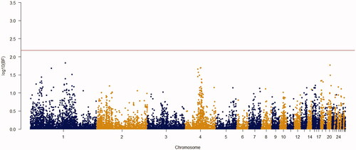
Figure 2. Manhattan plot of resulted from Bayes factors using BayesCπ methodology for body weight at week 3 in the chicken F2 population. The y-axes indicate the logarithm (base 10) of Bayes factors and the x-axes indicate the position of SNPs along the genome in different chromosome numbers. A significant threshold is the base 10 logarithm of Bayes factor equal to 150.

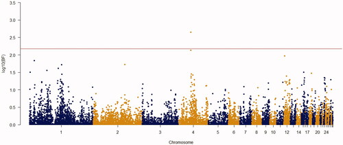
Figure 3. Manhattan plot of resulted from Bayes factors using BayesCπ methodology for body weight at week 4 in the chicken F2 population. The y-axes indicate the logarithm (base 10) of Bayes factors and the x-axes indicate the position of SNPs along the genome in different chromosome numbers. A significant threshold is the base 10 logarithm of Bayes factor equal to 150.

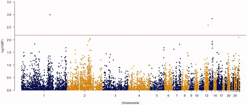
Figure 4. Manhattan plot of resulted from Bayes factors using BayesCπ methodology for body weight at week 5 in the chicken F2 population. The y-axes indicate the logarithm (base 10) of Bayes factors and the x-axes indicate the position of SNPs along the genome in different chromosome numbers. A significant threshold is the base 10 logarithm of Bayes factor equal to 150.

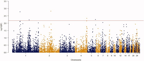
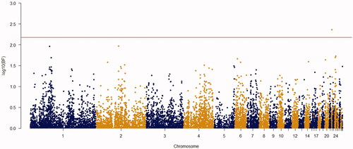
Figure 5. Manhattan plot of resulted from Bayes factors using BayesCπ methodology for body weight at week 6 in the chicken F2 population. The y-axes indicate the logarithm (base 10) of Bayes factors and the x-axes indicate the position of SNPs along the genome in different chromosome numbers. A significant threshold is the base 10 logarithm of Bayes factor equal to 150.

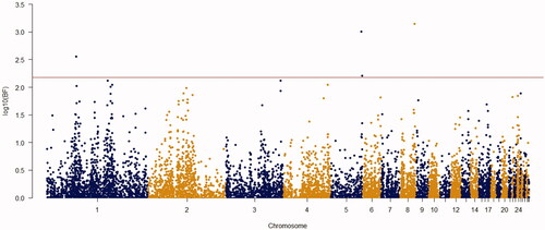
Figure 6. Manhattan plot of resulted from Bayes factors using BayesCπ methodology for body weight at week 7 in the chicken F2 population. The y-axes indicate the logarithm (base 10) of Bayes factors and the x-axes indicate the position of SNPs along the genome in different chromosome numbers. A significant threshold is the base 10 logarithm of Bayes factor equal to 150.

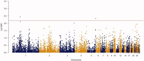
Figure 7. Manhattan plot of resulted from Bayes factors using BayesCπ methodology for body weight at week 8 in the chicken F2 population. The y-axes indicate the logarithm (base 10) of Bayes factors and the x-axes indicate the position of SNPs along the genome in different chromosome numbers. A significant threshold is the base 10 logarithm of Bayes factor equal to 150.

To identify genes surrounding each significant SNP we considered 0.5 Mbp up and downstream of the significant SNPs (SNP position ±0.25 Mb). In some cases, the significant SNPs were inside Genes and in some other cases, we presented the nearest gene to the identified SNP (Table 2).

Table 2. Significant SNPs, positions, and related genes associated with body weight at 2–9 weeks of ages. Gallus_gallus_5.0 (GCA_000002315.3).

Birds age	SNP ID	Chr	Position (bp)	Nearest Gene	Distance
BW3	Gga_rs14453946	4	38536266	DKK2	2 Kb D
BW3	Gga_rs312288120	4	38295506	LEF1	87.8 Kb D
BW4	Gga_rs13934188	1	123148233	LOC101751953	0
BW4	Gga_rs14998801	13	14041722	RASGEF1C	9 Kb U
BW4	Gga_rs313892216	12	15998199	FOXP1	0
BW5	Gga_rs314085832	2	86159751	LPCAT1	2 Kb D
BW5	GGa_rs315478364	1	56522937	AKR1D1	83.8 Kb D
BW5	Gga_rs314695269	5	58320627	GPR137C	0
BW5	Gga_rs14502415	4	86852277	EIF2AK3	134.8 Kb D
BW5	Gga_rs13934188	1	123148233	LOC101751953	0
BW6	Gga_rs14657039	8	28000752	ROR1	0
BW6	Gga_rs314695269	5	58320627	GPR137C	0
BW6	Gga_rs315478364	1	56522937	AKR1D1	83.8 Kb D
BW7	Gga_rs315478364	1	56522937	AKR1D1	83.8 Kb D
BW7	Gga_ rs14558098	5	59440955	LRFN5	178.5 Kb U
BW8	Gga_rs15998756	22	1397579	XPO7	0

SNP ID: Single nucleotide polymorphism id; Chr: Chromosome; BW: Body Weight.

DKK2: Dickkopf WNT Signalling Pathway Inhibitor 2; LEF1: Lymphoid Enhancer Binding Factor 1; RASGEF1C = RasGEF Domain Family Member 1 C; FOXP1: Forkhead Box P1; LPCAT1: Lysophosphatidylcholine Acyltransferase 1; AKR1D1: Aldo-Keto Reductase Family 1 Member D1; GPR137C = G Protein-Coupled Receptor 137 C; EIF2AK3: Eukaryotic Translation Initiation Factor 2 Alpha Kinase 3; ROR1: Receptor Tyrosine Kinase Like Orphan Receptor 1; LRFN5: Leucine Rich Repeat And Fibronectin Type III Domain Containing 5; XPO7: Exportin-7.

^U and ^D refers to upstream and downstream of gene.

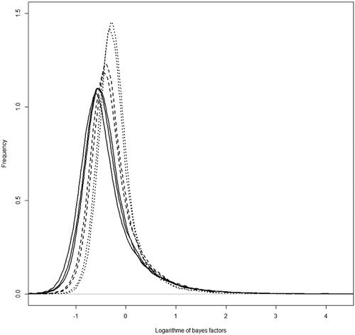
Beside significant SNPs that passed the significant threshold, an overall view of the distribution of Bayes factors across different weeks showed that the density of SNP effects shifts from around zero in early ages of weeks 2 and 3, and reaches its most distance from zero in weeks 4, 5 and 6 (Figure 8). Surprisingly these ages are the market goal ages in commercial broilers nowadays. After these ages, the distribution of Bayes factors shifts slightly back towards zero in weeks 7 and 8. Results show that the selection for market weight may be the main driver for the size of SNPs effects of different ages. So, the presence of markers with a larger effect sizes (more deviation from zero) was considered as evidence of the selection signature.

Figure 8. The probability density function of the logarithm of Bayes factors for SNPs effects in different ages. Dotted lines are referred to the weeks 2 and 3. Solid lines referred to the weeks 4, 5, and 6, and the dashed line referred to the weeks 7 and 8.

Discussion

No significant marker found for body weight at week 2 of age. According to Calborg et al. (2004) non-additive effect contribution at an early age can be considerable, therefore with models accounting for only additive effects failing to detect significant merkers are expected.

Since the present study is only looking for additive effects for the SNPs then the results are comparable with additive model in Carlborg et al. (2004). Frequency distribution of the significant SNPs over the weeks under study showed that the number and the effect sizes of SNPs increasing from early age to the week 5, which reaches its maximum of five significant SNPs and decreasing again weekly to reach its minimum of only one significant SNPs in week 8. This pattern may show the effect of artificial selection that pressures on these ages (weeks 5 and 6) for commercial and market purposes. Selection process may lead to skewed distributions or some significant deviation from mean effect (Pérez-Rodríguez et al. 2018). Signatures of selection (SOS) have the potential to elucidate the characteristics of genes and mutations associated with phenotypic traits. Additionally, genetic diversity, the essential material for breeding programs can be investigated by SOS analysis. Therefore, SOS has practical implications for the implementation of genomic prediction and genomic selection. As Bayesian models by introducing the global and local parameters, which can shrink the effects of some markers to zero and allow large effect markers to escape from the shrinkage it can be considered as an efficient and alternative model for genomic prediction (Habier et al. 2011).

Results showed that chromosome 4 is the second important chromosome in terms of the number of significant SNPs. Chromosome 4 explains a relatively high proportion of the growth variation observed in different ages (Podisi et al. 2013), which is in agreement with our results. Therefore, there is likely to be the key genes related to growth traits on this chromosome.

In this study, most significant markers (9 SNPs) were located on macro chromosomes (GGA1, GGA2, GGA4, GGA5) which is an indication of the higher contributions of these chromosomes to body weight traits (Xie et al. 2012).

Chromosome 1 reported as the main chromosome hosting several QTLs affecting body, breast muscle, thigh, and wings weights as well as overall growth (Rao et al. 2007). Among the significant markers, Gga_rs315478364 located on chromosome 1, was significant for body weights at three different ages (weeks 5, 6, and 7). This marker is located 83.8 Kb downstream of the AKR1D1 gene. Besides, Gga_rs13934188 located on the same chromosome was significant for two different ages (weeks 4 and 5). This marker is located within the LOC101751953 gene, which is one of the non-coding genes. These two markers are located in a relatively small distance from each other (∼10 Mb) that could be an indication of QTL presence in this region as declared by previous studies (Nadaf et al. 2009).

The genomic region between 38.29 Mbp and 46.9 Mbp on chromosome 4 is reported as an effective region on body weight for early ages (Sewalem et al. 2002). Although there was no significant SNP having Bayes factor greater than 150 in this region there were 7 SNPs with Bayes factor of 20–150 for week 2 which provides strong evidence of significance for this trait. It seems the interference of non-additive causes has the main responsibility to prevent SNSs located in this region passing the Bayes factor of 150.

As shown in Table 2, different genes of various metabolic pathways were identified, indicating a polygenic background of body weight. These genes were classified into five categories according to their metabolic functions. These categories are involved in signalling Wnt genes (DKK2, LEF-1, ROR-1), biosynthesis of various compounds, and metabolism (LPCAT1, AKR1D1, EIF2AK3), development of the nervous system (FOXP1, LRFN5), and transferring nuclear materials (XPO7). The last category including RASGEF1C and GPR137C genes play roles in internal and external cell transfer (protein transport through the membrane and intracellular vesicle transportation, and controls the cell vital processes including protein biosynthesis, differentiation and growth, cellular signalling, cell proliferation, stimulation cell growth, and tissue regeneration.

The FOXP1 gene plays solely in the development of the nervous system and cooperates with other family members of FOXP genes in developing other organs (Cheng et al. 2007). Also XPO7 plays a key role to facilitate the nuclear transfer of the thyroid hormone receptor (TR) gene (Stern 2015). TR is the main receptor of the T₃ hormone which regulates the metabolism and growth rate. Additionally, it plays critical roles in neurodevelopment, the development of lung, skeletal, and bone mass.

Wnt signalling genes play role in embryonic development. Currently, Wnt proteins are known as a major family of growth signalling molecules (Cadigan and Liu 2006). These genes encode diverse families of secreted lipid-modified signalling proteins that are required during the body development (Clevers 2006), osteogenesis (Li et al. 2005), the regulation of cartilage development and foetal growth (Surmann-Schmitt et al. 2009). Also, the activation of canonical Wnt signalling is recognised as an important mechanism for vascular development (Goodwin et al. 2006). Wnt receptors through cooperating with TGF-β, regulate cell fate and proliferation during development and tissue homeostasis (Barker et al. 1999). Wnt signalling extracellular activity is regulated by Dkk family factors (Surmann-Schmitt et al. 2009). Binding DKK2 gene to LRP5/LRP6 through forming a ternary complex with trans-membrane proteins regulates the canonical Wnt pathway. Canonical Wnt signalling stimulates osteogenesis, and Dkk2 gene is involved in late stages of osteoblast differentiation into mineralised matrices. During this time Wnt7b expression reaches its peak level. Dkk2 deficiency in vitro affected osteocalcin and osteopontin expression considerably (Li et al. 2005). Osteocalcin is secreted by osteoblasts and it is implicated in bone mineralisation and calcium ion homeostasis. Osteopontin helps to myogenic differentiation and finally muscle regeneration (Uaesoontrachoon et al. 2008). Following the consecutive transition of growth signals, Wnt can induce the transcriptional activity of numerous developmental genes through the activation of β-catenin/LEF-1 complexes in the nucleus (Filali et al. 2002). Members of the LEF1/TCF family of transcriptional factors can activate the transcription of genes by interacting with β-catenin (a downstream component of the Wnt signalling pathway) (Barker et al. 1999). The importance of LEF performance in Wnt signalling has long been proven in multiple developments and morphogenesis models (Filali et al. 2002). RORs genes are members of the nuclear receptor family of intracellular transcription factors that can be considered as the main regulators of Wnt signalling non-canonical pathways. These pathways are activated via the binding of Wnt to the frizzled domain and RORs as co-receptor. ROR-1 is a member of the ROR family of tyrosine kinase-like receptors that are highly conserved between various species (Rodriguez-Niedenführ et al. 2004). Receptor tyrosine kinases (RTKs) play an important role in many cellular processes, including differentiation, proliferation, and cell migration, angiogenesis, and survival (Green et al. 2008). In humans, skeletal development is known as the fundamental performance of ROR proteins (Green et al. 2008). Some studies have shown ROR1 signalling is involved in late limb development compared to early limb development (Rodriguez-Niedenführ et al. 2004).

The second group including LPCAT1, AKR1D1, EIF2AK3 genes have an important role in growth by participating in the biosynthesis and metabolism of various substances. Steroid 5β-reductase (AKR1D1) is a member of the Aldo keto reductase (AKR) (Mindnich et al. 2011) enzyme. This enzyme is required for the metabolism of hormones such as androgen, oestrogen, progesterone, and also prostaglandins (Seery et al. 1998). Furthermore, the main physiological function of AKR1D1 is participation in the biosynthesis of bile acids that is known as an important metabolic pathway in all vertebrates (Mindnich et al. 2011). Steroid hormones such as oestrogens and androgens have been raised as the main growth factor simulators. Oestrogens regulate metabolic activity of growth hormone (GH) either in the secretion or in the action levels (Leung et al. 2004). Oestrogens also can affect the pituitary secretion of GH. Moreover, it specifically can increase the expression of the suppressor cytokine signalling 2 that is a negative regulator of the GHR-JAK2-STAT5 signalling pathways (Rico-Bautista et al. 2006). On the other hand, Bile acids have a critical function to digestion and absorption of dietary fat and fat-soluble vitamins, due to forming mixed micelles in the small intestine.

EIF2AK3 membrane protein acts as a sensor to regulate the total protein synthesis. It is also essential for the normal turnover of insulin secretion from beta cells and bone growth (Liu et al. 2012). Insulin is a hormone that plays a key role in metabolism. It also involves in the storage of glycogen in muscles and amino acid transferring of the skeletal muscle system. This hormone has a GH-like act through increasing the consumption of amino acids and exchanging them to proteins and preventing degradation of available proteins in cells. Insulin is involved to transfer the received carbohydrate by the muscles. In this way, it plays an important role to build a muscular body (Ghorbani and Hashtrodi 2014).

Finally, comparing the compressed mixed linear model used by Emrani et al., in 2017 and a recent study represented the complete differences in terms of potential candidate genes resulted from these different methodologies. As expected, no commonness can be seen in this comparison. 10 candidate genes reported by Emrani et al., in 2017 included DIS3, BORA, UBE2H, CNOT10, SGOL1, ADGRB3, DTNB, SETD3, EFNA5, and SPINZ (Emrani et al. 2017) however, the recent study detected 16 candidate genes including DKK2, LEF1, RASGEF1C, FOXP1, LPCAT1, AKR1D1, GPR137C, EIF2AK3, ROR1, AKR1D1, LRFN5, XPO7, LOC101751953 and LOC101751953.

Conclusions

Our results have provided a list of candidate genes for body weight at ages 2–8 weeks. Results can be used in genomic selection and marker or gene assisted selection to improve growth rate in chicken. Macro chromosomes showed a remarkable role in growth control. According to the obtained results, GGA1 and GGA4 are the most important chromosomes that contain QTLs associated with the growth traits in the chicken genome. On the other hand, there were different genetic regions responsible for early and late ages for the observed traits. Ages of 4, 5, and 6 had the highest number of significant SNPs, and weeks 2 and 3 had the lowest number of significant SNPs. It may be due to the effect of non-additive drivers or due to selection goals for broilers which are weeks 4, 5, and 6 in modern commercial broiler types. This conclusion confirmed by drawing the overall density of all SNPs effects of different ages. The difference in the number of significant SNPs in different ages indicates the effect of artificial selection, which admit the breeding has been working properly in the chicken groups for the ages of importance. This is important as such that different regions in the genome may cause the trait of interest in different stages of life time.

It shows that the density of SNPs effects for the intended market ages is more segregating than other ages.

Ethical approval

All experimental procedures have been approved by the Animal Care Committee of Tarbiat Modares University with a letter number 1229734.

Acknowledgements

The authors gratefully acknowledge to Dr. Rasoul Vaez torshizi from Tarbiat Modares University, Iran, for the study design and collection of phenotypic data. Sincere gratitude to Dr. Just Jensen from Aarhus University for scientific assistance and supporting genotyping the birds. Thanks to Staff of Arian Line Breeding Center and West Azarbayjan Native Fowls Breeding Center for providing parents of F1 chickens. The main financial support came from Tarbiat Modares University and the genotyping of the birds was supported by Aarhus University, Denmark by GenSAP Grant no 0603-00519B from the Danish Innovation.

Disclosure statement

No potential conflict of interest was reported by the author(s).

Data and model availability statement

phenotypes: https://figshare.com/articles/Phenotypes_rar/11369358/1

genotypes: https://figshare.com/articles/f2_chicken_data/11369352/2

Additional information

Funding

The main financial support came from Tarbiat Modares University and the genotyping of the birds was supported by Aarhus University, Denmark by GenSAP Grant no 0603-00519B from the Danish Innovation.

References

- Anderegg A, Lin H-P, Chen J-A, Caronia-Brown G, Cherepanova N, Yun B, Joksimovic M, Rock J, Harfe BD, Johnson R, et al. 2013. An Lmx1b-miR135a2 regulatory circuit modulates Wnt1/Wnt signaling and determines the size of the midbrain dopaminergic progenitor pool. PLoS Genet. 9(12):e1003973.
- Barker N, Morin PJ, Clevers H. 1999. The Yin-Yang of TCF/β-catenin signaling. Adv Cancer Res. 77:1–24.
- Begli HE, Torshizi RV, Masoudi AA, Ehsani A, Jensen J. 2017. Relationship between residual feed intake and carcass composition, meat quality and size of small intestine in a population of F2 chickens. Livest Sci. 205:10–15.
- Cadigan KM, Liu YI. 2006. Wnt signaling: complexity at the surface. J Cell Sci. 119(Pt 3):395–402.
- Carlborg Ö, Hocking PM, Burt DW, Haley CS. 2004. Simultaneous mapping of epistatic QTL in chickens reveals clusters of QTL pairs with similar genetic effects on growth. Genet Res. 83(3):197–209.
- Cheng L, Chong M, Fan W, Guo X, Zhang W, Yang X, Liu F, Gui Y, Lu D. 2007. Molecular cloning, characterization, and developmental expression of foxp1 in zebrafish. Dev Genes Evol. 217(10):699–707.
- Clevers H. 2006. Wnt/beta-catenin signaling in development and disease. Cell. 127(3):469–480.
- Costa RB, Camargo GM, Diaz ID, Irano N, Dias MM, Carvalheiro R, Boligon AA, Baldi F, Oliveira HN, Tonhati H. 2015. Genome-wide association study of reproductive traits in Nellore heifers using Bayesian inference. Genet Sel Evol. 47:1–9.
- Emrani H, Torshizi RV, Masoudi AA, Ehsani A. 2017. Identification of new loci for body weight traits in F2 chicken population using genome-wide association study. Livest Sci. 206:125–131.
- Filali M, Cheng N, Abbott D, Leontiev V, Engelhardt JF. 2002. Wnt-3A/beta-catenin signaling induces transcription from the LEF-1 promoter. J Biol Chem. 277(36):33398–33410.
- Fu, W., Dekkers, J.C., Lee, W.R. et al. Linkage disequilibrium in crossbred and pure line chickens. Genet Sel Evol 47, 11 (2015). https://doi.org/https://doi.org/10.1186/s12711-015-0098-4
- Ghorbani M, Hashtrodi R. 2014. Insulın hormone effects on Ft&St muscles of body bulding athlets and diabetic people type. ISSCS. 2(5):826–835.
- Goddard ME, Hayes BJ. 2009. Mapping genes for complex traits in domestic animals and their use in breeding programmes. Nat Rev Genet. 10(6):381–391.
- Goodwin AM, Sullivan KM, D’Amore PA. 2006. Cultured endothelial cells display endogenous activation of the canonical Wnt signaling pathway and express multiple ligands, receptors, and secreted modulators of Wnt signaling. Dev Dyn. 235(11):3110–3120.
- Green JL, Kuntz SG, Sternberg PW. 2008. Ror receptor tyrosine kinases: orphans no more. Trends Cell Biol. 18(11):536–544.
- Habier D, Fernando RL, Kizilkaya K, Garrick DJ. 2011. Extension of the Bayesian alphabet for genomic selection. BMC Bioinform. 1:12–186.
- Kang HM, Sul JH, Service SK, Zaitlen NA, Kong SY, Freimer NB, Sabatti C, Eskin E. 2010. Variance component model to account for sample structure in genome-wide association studies. Nat Genet. 42(4):348–354.
- Kass R, Raftery A. 1995. Bayes factors. J Am Stat Assoc. 90 (430):773–795.
- Kim K, Jung J, Caetano-Anollés K, Sung S, Yoo DAhn, Choi B-H, Kim H-C, Jeong J-Y, Cho Y-M, Park E-W, et al. 2018. Artificial selection increased body weight but induced increase of runs of homozygosity in Hanwoo cattle. PLoS One. 13(3):e0193701.
- Ledur M, Navarro N, Pérez-Enciso M. 2010. Large-scale SNP genotyping in crosses between outbred lines: how useful is it? Heredity (Edinb). 105(2):173–182.
- Legarra, A., Ricard, A., and Filangi, O. (2011). GS3: Genomic Selection, Gibbs Sampling, Gauss-Seidel (and BayesCπ). Paris, France: INRA.
- Leung K-C, Johannsson G, Leong GM, Ho KK. 2004. Estrogen regulation of growth hormone action. Endocr Rev. 25(5):693–721.
- Li X, Liu P, Liu W, Maye P, Zhang J, Zhang Y, Hurley M, Guo C, Boskey A, Sun L, et al. 2005. Dkk2 has a role in terminal osteoblast differentiation and mineralized matrix formation. Nat Genet. 37(9):945–952.
- Liu J, Hoppman N, O'Connell JR, Wang H, Streeten EA, McLenithan JC, Mitchell BD, Shuldiner AR. 2012. A functional haplotype in EIF2AK3, an ER stress sensor, is associated with lower bone mineral density. J Bone Miner Res. 27(2):331–341.
- Madsen P, Jensen J. 2002. A package for analysing multivariate mixed models. Tjele (Denmark): Danish Institute of Agricultural Sciences (DIAS).
- Maher B. 2008. Personal genomes: the case of the missing heritability. Nature. 456(7218):18–21.
- Maher B. 2008. The case of the missing heritability: when scientists opened up the human genome, they expected to find the genetic components of common traits and diseases. But they were nowhere to be seen. Brendan Maher shines a light on six places where the missing loot could be stashed away. Nature. 456: 18–22.
- Mindnich R, Drury JE, Penning TM. 2011. The effect of disease associated point mutations on 5β-reductase (AKR1D1) enzyme function. Chem Biol Interact. 191(1–3):250–254.
- Nadaf J, Pitel F, Gilbert H, Duclos MJ, Vignoles F, Beaumont C, Vignal A, Porter TE, Cogburn LA, Aggrey SE, et al. 2009. QTL for several metabolic traits map to loci controlling growth and body composition in an F2 intercross between high- and low-growth chicken lines. Physiol Genomics. 38(3):241–249.
- Pérez-Rodríguez P, Acosta-Pech R, Pérez-Elizalde S, Cruz CV, Espinosa JS, Crossa J. 2018. A Bayesian genomic regression model with skew normal random errors. G3 (Bethesda). 8(5):1771–1785. 8:
- Peters S, Kizilkaya K, Garrick D, Fernando R, Reecy J, Weaber R, Silver G, Thomas M. 2012. Bayesian genome-wide association analysis of growth and yearling ultrasound measures of carcass traits in Brangus heifers. J Anim Sci. 90(10):3398–3409.
- Podisi BK, Knott SA, Burt DW, Hocking PM. 2013. Comparative analysis of quantitative trait loci for body weight, growth rate and growth curve parameters from 3 to 72 weeks of age in female chickens of a broiler-layer cross. BMC Genet. 14:11–22.
- Rao Y, Shen X, Xia M, Luo C, Nie Q, Zhang D, Zhang X. 2007. SNP mapping of QTL affecting growth and fatness on chicken GGA1. Genet Sel Evol. 39(5):569–582.
- Rico-Bautista E, Flores-Morales A, Fernández-Pérez L. 2006. Suppressor of cytokine signaling (SOCS) 2, a protein with multiple functions. Cytokine Growth Factor Rev. 17(6):431–439.
- Rodriguez-Niedenführ M, Pröls F, Christ B. 2004. Expression and regulation of ROR-1 during early avian limb development. Anat Embryol (Berl). 207(6):495–502.
- Seery L, Nestor P, FitzGerald G. 1998. Molecular evolution of the aldo-keto reductase gene superfamily. J Mol Evol. 46(2):139–146.
- Sewalem A, Morrice D, Law A, Windsor D, Haley C, Ikeobi C, Burt D, Hocking P. 2002. Mapping of quantitative trait loci for body weight at three, six, and nine weeks of age in a broiler layer cross. Poult Sci. 81(12):1775–1781.
- Stern MER. 2015. The impact of the ubiquitin-proteasome pathway and CRM1-independent exportins on thyroid hormone receptor localization and the expression of T3-responsive genes [M.Sc. thesis]. Williamsburg (VA): College of William and Mary.
- Surmann-Schmitt C, Widmann N, Dietz U, Saeger B, Eitzinger N, Nakamura Y, Rattel M, Latham R, Hartmann C, von der Mark H, et al. 2009. Wif-1 is expressed at cartilage-mesenchyme interfaces and impedes Wnt3a-mediated inhibition of chondrogenesis. J Cell Sci. 122(Pt 20):3627–3637.
- Uaesoontrachoon K, Yoo H-J, Tudor EM, Pike RN, Mackie EJ, Pagel CN. 2008. Osteopontin and skeletal muscle myoblasts: association with muscle regeneration and regulation of myoblast function in vitro. Int J Biochem Cell Biol. 40(10):2303–2314.
- van den Berg I, Fritz S, Boichard D. 2013. QTL fine mapping with Bayes C (π): a simulation study. Genet Sel Evol. 45:1–11.
- Wakefield J. 2009. Bayes factors for genome-wide association studies: comparison with p-values. Genet Epidemiol. 33(1):79–86.
- Walugembe M, Bertolini F, Dematawewa CMB, Reis MP, Elbeltagy AR, Schmidt CJ, Lamont SJ, Rothschild MF. 2018. Detection of selection signatures Among Brazilian, Sri Lankan, and Egyptian chicken populations under different environmental conditions. Front Genet. 9:737.
- Weng Z, Xu Y, Li W, Chen J, Zhong M, Zhong F, Du B, Zhang B, Huang X. 2020. Genomic variations and signatures of selection in Wuhua yellow chicken. PLoS One. 15(10):e0241137.
- Wilson MA, Iversen ES, Clyde MA, Schmidler SC, Schildkraut JM. 2010. Bayesian model search and multilevel inference for Snp association studies. Ann Appl Stat. 4(3):1342–1364.
- Xie L, Luo C, Zhang C, Zhang R, Tang J, Nie Q, Ma L, Hu X, Li N, Da Y, et al. 2012. Genome-wide association study identified a narrow chromosome 1 region associated with chicken growth traits. PLoS One. 7(2):e30910
- Zhang Z, Ersoz E, Lai CQ, Todhunter RJ, Tiwari HK, Gore MA, Bradbury PJ, Yu J, Arnett DK, Ordovas JM, et al. 2010. Mixed linear model approach adapted for genome-wide association studies. Nat Genet. 42(4):355–360.