Virtual internal model tuning for cascade control systems

ABSTRACT

Cascade control is used in many practical applications. To realize the desired specification of the cascade control systems, accurate mathematical models of the plant are not only inner but also outer loops required. However, there are also many situations where it is difficult to execute ideal experiments for obtaining mathematical models for practical reasons. In such situations, it is expected that the direct usage of the data for control design enables us to obtain desired controllers. From these backgrounds, we propose a controller tuning method for the two controllers in a cascade control system. Here, we apply virtual internal model tuning proposed by the authors to update the cascade control system. In this proposed method, specifications of the inner and the outer loops can be set independently. The optimal parameters of the controller in each loop can be obtained using the least square method. Finally, the validity and usefulness of the proposed method are illustrated using experiments.

KEYWORDS:

• Cascade control system
• controller design
• data-driven control
• virtual internal model tuning

1. Introduction

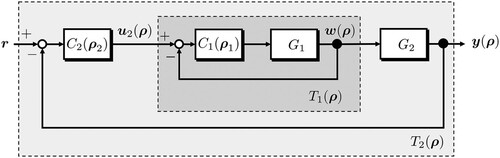
The cascade control system [1] is used in various practical applications, such as in chemical plants and motor control. The typical block diagram of the cascade control system is shown in Figure 1, where the dark grey box with a broken line is the inner loop, whereas the light grey box is the outer loop. Using these two controllers, the behaviour of the inner and outer loops can be designed separately. Particularly, by considering the control target as a cascade coupling, the control system can be designed to easily improve the control performance. By designing the characteristics of the inner loop to move faster than those of the outer loop, a better control performance can be obtained, which is difficult to design using a single controller.

Figure 1. The cascade control system.

Recently, several approaches to control system design with direct utilization of data without the mathematical model of a plant have been proposed and studied. These approaches are referred to as data-driven control, such as Iterative Feedback Tuning (IFT) in [2], Virtual Reference Iterative Tuning (VRFT) in [3], Fictitious Iterative Reference Tuning (FRIT) in [4]. VRFT and FRIT have practical advantages because they require only one-shot experimental data for offline optimization, whereas IFT requires many experiments. The authors have recently proposed a novel controller parameter tuning using only output data for a conventional feedback control system. This method is referred to as Virtual Internal Model Tuning (VIMT) in [5]. VIMT is a controller parameter tuning method that uses the output and the implemented initial controller instead of the input signal. We compare VIMT with other methods. FRIT includes the controller structure as an inverse direction in the cost function. Therefore, it requires nonlinear optimizations when only the numerator of the controller is parameterized, as in the case of a PID controller. VRFT includes the controller in the forward direction in the cost function; thus, the controller can be updated using linear optimization for PID controllers. However, VRFT assumes the use of a filter to enable computation because the original cost function is non-proper and the filter changes the tuning performance. VIMT outperforms FRIT and VRFT in terms of convenience in practical applications.

The reference [6–8] investigated on data-driven controller tuning for cascade control systems. In the VRFT-based method, the filters must be designed to calculate the cost function and the accuracy of the obtained parameter is degraded by the filter performance. FRIT requires the use of nonlinear optimization, which may cause the local optimum solution to converge. The optimization calculation method and filter design still have some shortcomings. Based on the aforementioned issues, the tuning cascade controller by VIMT is considered in this study. We propose a method that can independently tune the characteristics of the inner and outer loops. When using a controller with tunable parameters in the numerator, such as a PID controller, we propose that the two controllers can be obtained by linear optimization.

The remainder of this paper is arranged The remainder of this paper is arranged as follows: Section 2 presents the notation and problem setup; Section 3 explains the VIMT and Section 4 explains a VIMT-based tuning rule for cascade control systems; Section 5 presents the verification results using the cart system experimental equipment; finally, Section 6 summarizes the paper.

2. Preliminaries

2.1. Notations

Let ${\mathbb{R}}^n$ be the set of n-dimensional real column vectors and ${\mathit{a}}^{\mathrm{\top }}$ represents the transpose for $\mathit{a}\in {\mathbb{R}}^n$. The value at time k in the discrete time signal $\mathit{w}$ is denoted as $w_{\left[k\right]}$. The vector of the signal between k = 0 and k = N is denoted as ${\mathit{w}}_{[0,N]}$.Let z denote the shift operator defined as $z{w}_{\left[k\right]}=w_{[k+1]}$. The norm for this signal is defined as: (1) $\Vert \mathit{w}{\Vert }_{[0,N]}:=\sqrt{\sum _{i=0}^N{w}_{\left[k\right]}^2}.$(1) The output of a system with a transfer function G regarding the input $\mathit{w}$ should be denoted as the convolution form of the Markov parameter of G and $\mathit{w}$. However, we denote the output as $G\mathit{w}$ to enhance readability. The content of this research is discussed in discrete time; however, it can be discussed in continuous time as well. Moreover, discussions can be made using signals with a finite time span because G are linear time-invariant systems. We denote the finite time output of G with the input signal $\mathit{w}$ between k = 0 and k = k as $G{\mathit{w}}_{[0,k]}.$

2.2. Problem formulation

Consider a cascade control system shown in Figure 1. Plants $G_1$ and $G_2$ are linear, time-invariant, finite-dimensional, single-input, single-output, strictly proper, and minimum phase systems. Moreover, we assume that $G_1$ and $G_2$ are unknown, whereas their relative degrees are known. The inner and outer controllers $C_1$ and $C_2$ are described using tunable parameter vectors ${\mathit{\rho }}_1$ and ${\mathit{\rho }}_2$, respectively. The two controllers are denoted as (2) $\begin{array}{rl}{C}_i\left({\mathit{\rho }}_i\right)& :=\frac{{\rho }_{n_c^i+m_c^i}^i{q}^{m_c^i}+{\rho }_{n_c^i+m_c^i-1}^i{q}^{m_c^i-1}+\cdots +{\rho }_{n_c^i}^i}{z^{n_c}+{\rho }_{n_c^i-1}^i{z}^{n_c^i-1}+\cdots +{\rho }_0^i},\\ & (i=1,2)\end{array}$(2) with a parameter vector ${\mathit{\rho }}_i:=[{\rho }_0^i,{\rho }_1^i,\dots ,{\rho }_{n_c^i+m_c^i}^i{]}^{\mathrm{\top }}\in {\mathbb{R}}^{n_c^i+m_c^i+1}.$ We define $\mathit{\rho }:=\{{\mathit{\rho }}_1,{\mathit{\rho }}_2\}$ as the parameter vector of each of the two controllers $C_1\left({\mathit{\rho }}_1\right)$ and $C_2\left({\mathit{\rho }}_2\right)$, respectively. We assume that $C_1\left({\mathit{\rho }}_1^0\right)$ and $C_2\left({\mathit{\rho }}_2^0\right)$ have no unstable zero.

The transfer function from the reference signal $\mathit{r}$ to the output $\mathit{y}\left(\mathit{\rho }\right)$ is denoted as: (3) $T_2\left(\mathit{\rho }\right):=\frac{G_2{G}_1{C}_1\left({\mathit{\rho }}_1\right)C_2\left({\mathit{\rho }}_2\right)}{1+G_1{C}_1\left({\mathit{\rho }}_1\right)+G_2{G}_1{C}_1\left({\mathit{\rho }}_1\right)C_2\left({\mathit{\rho }}_2\right)},$(3) and the inner loop transfer function from ${\mathit{u}}_2$ to $\mathit{w}$ is denoted as: (4) $T_1\left(\mathit{\rho }\right):=\frac{G_1{C}_1\left({\mathit{\rho }}_1\right)}{1+G_1{C}_1\left({\mathit{\rho }}_1\right)}.$(4) Here, we provide a desired tracking reference model from $\mathit{r}$ to the output $\mathit{y}$ as $T_d$. Thus, the desired output is described as (5) ${\mathit{y}}_d:=T_d\mathit{r}.$(5) Under these settings, the problem considered here is to find a controller parameter $\mathit{\rho }:=\{{\mathit{\rho }}_1,{\mathit{\rho }}_2\}$ such that $\mathit{y}\left(\mathit{\rho }\right)$ follows the desired response ${\mathit{y}}_d:=T_d\mathit{r}$ without using models of $G_1$ and $G_2$.

3. Virtual internal model tuning

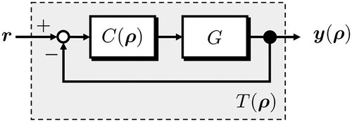
In this section, we explain virtual internal model tuning for a controller in the conventional closed-loop system [5]. Here, we consider a closed-loop system illustrated as Figure 2. In this figure, the feedback controller has some tunable parameters $\mathit{\rho }$ and it is written as $C\left(\mathit{\rho }\right)$. A plant G is a single input, single output, linear time invariant, and minimum phase system. The reference signal is denoted as $\mathit{r}$. The output is written as $\mathit{y}\left(\mathit{\rho }\right)$. A transfer function from r to $\mathit{y}\left(\mathit{\rho }\right)$ is denoted as $T\left(\mathit{\rho }\right)$ which is written as: (6) $T\left(\mathit{\rho }\right):=\frac{GC\left(\mathit{\rho }\right)}{1+GC\left(\mathit{\rho }\right)}.$(6) The objective of this control system is to ensure the output is close to a given desired output ${\mathit{y}}_d:=T_{d}r$. $\mathit{y}\left({\mathit{\rho }}^0\right)$ is assumed as the initial output, which is obtained from the closed loop with the initial controller $C\left({\mathit{\rho }}^0\right)$ embedded with the initial parameter ${\mathit{\rho }}^0$. Subsequently, we minimize (7) $\Vert y_d-T\left(\mathit{\rho }\right)r{\Vert }_{[0,N]}.$(7) To solve this problem, we express the output $\mathit{y}\left(\mathit{\rho }\right)$ using the initial information (8) $\mathit{y}(\mathit{\rho }{)}_{[0,N]}:=T(\mathit{\rho }\left)T\right({\mathit{\rho }}^0{)}^{-1}\mathit{y}({\mathit{\rho }}^0{)}_{[0,N]}.$(8) This problem aims to place $T\left(\mathit{\rho }\right)$ close to $T_d$ using tuning parameters. We assume that there exists a ${\mathit{\rho }}^{\ast }$ such that the system $T\left({\mathit{\rho }}^{\ast }\right)$ match to $T_d$ as (9) $T\left({\mathit{\rho }}^{\ast }\right)=\frac{GC\left({\mathit{\rho }}^{\ast }\right)}{1+GC\left({\mathit{\rho }}^{\ast }\right)}=T_d.$(9) After parameter tuning, we express G using $T_d$ and $C\left({\mathit{\rho }}^{\ast }\right)$ in Equation (9(9) $T\left({\mathit{\rho }}^{\ast }\right)=\frac{GC\left({\mathit{\rho }}^{\ast }\right)}{1+GC\left({\mathit{\rho }}^{\ast }\right)}=T_d.$(9) ). Then, substituting G into Equation (8(8) $\mathit{y}(\mathit{\rho }{)}_{[0,N]}:=T(\mathit{\rho }\left)T\right({\mathit{\rho }}^0{)}^{-1}\mathit{y}({\mathit{\rho }}^0{)}_{[0,N]}.$(8) ), the unknown desired output $\mathit{y}\left(\mathit{\rho }\right)$ and the desired controller $C\left({\mathit{\rho }}^{\ast }\right)$ can be expressed as follows: (10) $y({\mathit{\rho }}^{\ast }{)}_{[0,N]}=\{T_d+(1-T_d\left)\frac{C\left({\mathit{\rho }}^{\ast }\right)}{C\left({\mathit{\rho }}^0\right)}\right\}y({\mathit{\rho }}^0{)}_{[0,N]}$(10) without G. To obtain the unknown ${\mathit{\rho }}^{\ast }$, we replace ${\mathit{\rho }}^{\ast }$ by $\mathit{\rho }$ of Equation (10(10) $y({\mathit{\rho }}^{\ast }{)}_{[0,N]}=\{T_d+(1-T_d\left)\frac{C\left({\mathit{\rho }}^{\ast }\right)}{C\left({\mathit{\rho }}^0\right)}\right\}y({\mathit{\rho }}^0{)}_{[0,N]}$(10) ). Subsequently we rewrote $\mathit{y}\left(\mathit{\rho }\right)$ as $\tilde{y}\left(\mathit{\rho }\right)$. We then minimize the cost function (11) $J\left(\mathit{\rho }\right):=\Vert y_d-\tilde{y}\left(\mathit{\rho }\right){\Vert }_{[0,N]}.$(11) Finally, by implementing the optimal parameter (12) ${\mathit{\rho }}^{\ast }:=\mathrm{a}\mathrm{r}\mathrm{g}\underset{\mathit{\rho }}{min}J\left(\mathit{\rho }\right),$(12) the desired output ${\mathit{y}}_{d\left[k\right]}=y({\mathit{\rho }}^{\ast }{)}_{\left[k\right]}$ is achieved.

Figure 2. The conventional closed-loop system.

4. Virtual internal model tuning for the cascade system

In this section, we propose a tuning method using virtual internal model tuning for two controllers on the cascade control system in Figure 1.

4.1. Cost function

We assume that the output $\mathit{w}\left({\mathit{\rho }}_1^0\right)$ of the inner loop and the output $\mathit{y}\left({\mathit{\rho }}_1^0\right)$ of the outer loop are provided. Assume the desired specifications of the inner and outer loops are $T_{d1}$ and $T_{d2}$, respectively. Here, we consider updating the parameters in two controllers independently to achieve the specification for each loop. This problem aims to place $T_1\left(\mathit{\rho }\right)$ and $T_2\left(\mathit{\rho }\right)$ close to $T_{d1}$ and $T_{d2}$ by tuning parameters, respectively. That is, after tuning the parameter, it can be assumed as (13) $\begin{array}{rl}{T}_1\left({\mathit{\rho }}^{\ast }\right)& =\frac{G_1{C}_1\left({\mathit{\rho }}_1^{\ast }\right)}{1+G_1{C}_1\left({\mathit{\rho }}_1^{\ast }\right)}=T_{d1},\end{array}$(13) (14) $\begin{array}{rl}{T}_2\left({\mathit{\rho }}^{\ast }\right)& =\frac{T_{d1}{G}_2{C}_2\left({\mathit{\rho }}_2^{\ast }\right)}{1+T_{d1}{G}_2{C}_2\left({\mathit{\rho }}_2^{\ast }\right)}=T_{d2}\end{array}$(14) Here, we assume that there exist $T_{d1}$ and $T_{d2}$ such that Equations (13(13) $\begin{array}{rl}{T}_1\left({\mathit{\rho }}^{\ast }\right)& =\frac{G_1{C}_1\left({\mathit{\rho }}_1^{\ast }\right)}{1+G_1{C}_1\left({\mathit{\rho }}_1^{\ast }\right)}=T_{d1},\end{array}$(13) ) and (14(14) $\begin{array}{rl}{T}_2\left({\mathit{\rho }}^{\ast }\right)& =\frac{T_{d1}{G}_2{C}_2\left({\mathit{\rho }}_2^{\ast }\right)}{1+T_{d1}{G}_2{C}_2\left({\mathit{\rho }}_2^{\ast }\right)}=T_{d2}\end{array}$(14) ) are completely satisfied. In reality, such $T_{d1}$ and $T_{d2}$ cannot be set because $G_1$ and $G_2$ are unknown. Therefore, since the relative orders of $G_1$ and $G_2$ are known, we consider setting $T_{d1}$ and $T_{d2}$ to match the relative orders in Equations (13(13) $\begin{array}{rl}{T}_1\left({\mathit{\rho }}^{\ast }\right)& =\frac{G_1{C}_1\left({\mathit{\rho }}_1^{\ast }\right)}{1+G_1{C}_1\left({\mathit{\rho }}_1^{\ast }\right)}=T_{d1},\end{array}$(13) ) and (14(14) $\begin{array}{rl}{T}_2\left({\mathit{\rho }}^{\ast }\right)& =\frac{T_{d1}{G}_2{C}_2\left({\mathit{\rho }}_2^{\ast }\right)}{1+T_{d1}{G}_2{C}_2\left({\mathit{\rho }}_2^{\ast }\right)}=T_{d2}\end{array}$(14) ), respectively. In addition, if tracking to a step signal, for example, is considered as a tuning specification for both, a condition is added as appropriate so that $T_{d2}\left(0\right)=1$ is satisfied. In the actual control target, mechanical limitations such as input conditions must be considered. Therefore, the time constant of the first-order delay system, for example, should not be overly tight, but should be determined within the range achievable by the target system. For this study, we consider the situation where appropriate tuning specifications are given.

From Equation (13(13) $\begin{array}{rl}{T}_1\left({\mathit{\rho }}^{\ast }\right)& =\frac{G_1{C}_1\left({\mathit{\rho }}_1^{\ast }\right)}{1+G_1{C}_1\left({\mathit{\rho }}_1^{\ast }\right)}=T_{d1},\end{array}$(13) ), $G_1$ can be written as (15) $G_1=\frac{T_{d1}}{(1-T_{d1})C_1\left({\mathit{\rho }}_1^{\ast }\right)}.$(15) From Equation (14(14) $\begin{array}{rl}{T}_2\left({\mathit{\rho }}^{\ast }\right)& =\frac{T_{d1}{G}_2{C}_2\left({\mathit{\rho }}_2^{\ast }\right)}{1+T_{d1}{G}_2{C}_2\left({\mathit{\rho }}_2^{\ast }\right)}=T_{d2}\end{array}$(14) ), $G_2$ can be expressed as (16) $G_2=\frac{T_{d2}}{(1-T_{d2})T_{d1}{C}_2\left({\mathit{\rho }}_2^{\ast }\right)}.$(16) To achieve the desired output ${\mathit{y}}_d$, we express the output $\mathit{y}\left(\mathit{\rho }\right)$ using only the provided information; the output can be expressed using the inverse system of $T_2\left({\mathit{\rho }}^0\right)$ as (17) $\mathit{y}({\mathit{\rho }}^{\ast }{)}_{[0,N]}:=T_2({\mathit{\rho }}^{\ast }\left)T_2\right({\mathit{\rho }}^0{)}^{-1}\mathit{y}({\mathit{\rho }}^0{)}_{[0,N]}.$(17) Using the relation (18) $\mathit{y}=G_2\mathit{w},$(18) $\mathit{y}\left({\mathit{\rho }}^{\ast }\right)$ can also be expressed as (19) $\begin{array}{rl}& \mathit{y}({\mathit{\rho }}^{\ast }{)}_{[0,N]}\\ & =T_{d2}(1+\frac{1}{G_2{C}_2\left({\mathit{\rho }}^0\right)}+\frac{1}{G_2{G}_1{C}_1\left({\mathit{\rho }}_1^0\right)C_2\left({\mathit{\rho }}_2^0\right)})\\ & \times \mathit{y}({\mathit{\rho }}^0{)}_{[0,N]}\end{array}$(19) (20) $\begin{array}{rl}& =T_{d2}\mathit{y}({\mathit{\rho }}^0{)}_{[0,N]}+\frac{T_{d2}}{C_2\left({\mathit{\rho }}^0\right)}\mathit{w}({\mathit{\rho }}^0{)}_{[0,N]}\\ & +\frac{T_{d2}}{G_1{C}_1\left({\mathit{\rho }}_1^0\right)C_2\left({\mathit{\rho }}_2^0\right)}\mathit{w}({\mathit{\rho }}^0{)}_{[0,N]}\end{array}$(20) By substituting Equation (15(15) $G_1=\frac{T_{d1}}{(1-T_{d1})C_1\left({\mathit{\rho }}_1^{\ast }\right)}.$(15) ) into $G_1$ in Equation (19(19) $\begin{array}{rl}& \mathit{y}({\mathit{\rho }}^{\ast }{)}_{[0,N]}\\ & =T_{d2}(1+\frac{1}{G_2{C}_2\left({\mathit{\rho }}^0\right)}+\frac{1}{G_2{G}_1{C}_1\left({\mathit{\rho }}_1^0\right)C_2\left({\mathit{\rho }}_2^0\right)})\\ & \times \mathit{y}({\mathit{\rho }}^0{)}_{[0,N]}\end{array}$(19) ), we obtain (21) $\begin{array}{rl}\mathit{y}({\mathit{\rho }}^{\ast }{)}_{[0,N]}& =T_{d2}\mathit{y}({\mathit{\rho }}^0{)}_{[0,N]}+\frac{T_{d2}}{C_2\left({\mathit{\rho }}^0\right)}\mathit{w}({\mathit{\rho }}^0{)}_{[0,N]}\\ & +\frac{(1-T_{d1})T_{d2}}{T_{d1}{C}_1\left({\mathit{\rho }}_1^0\right)C_2\left({\mathit{\rho }}_2^0\right)}{C}_1\left({\mathit{\rho }}_1^{\ast }\right)w({\mathit{\rho }}^0{)}_{[0,N]}.\end{array}$(21) To obtain ${\mathit{\rho }}^{\ast }$, we redefine the signal $\tilde{\mathit{y}}({\mathit{\rho }}_1{)}_{[0,N]}$ from Equation (21(21) $\begin{array}{rl}\mathit{y}({\mathit{\rho }}^{\ast }{)}_{[0,N]}& =T_{d2}\mathit{y}({\mathit{\rho }}^0{)}_{[0,N]}+\frac{T_{d2}}{C_2\left({\mathit{\rho }}^0\right)}\mathit{w}({\mathit{\rho }}^0{)}_{[0,N]}\\ & +\frac{(1-T_{d1})T_{d2}}{T_{d1}{C}_1\left({\mathit{\rho }}_1^0\right)C_2\left({\mathit{\rho }}_2^0\right)}{C}_1\left({\mathit{\rho }}_1^{\ast }\right)w({\mathit{\rho }}^0{)}_{[0,N]}.\end{array}$(21) ), by replacing ${\mathit{\rho }}^{\ast }$ with the tunable parameter $\mathit{\rho }$ and determine a cost function as follows: (22) $J_1\left({\mathit{\rho }}_1\right):=\Vert {\mathit{y}}_d-\tilde{\mathit{y}}\left({\mathit{\rho }}_1\right){\Vert }_{[0,N]}.$(22) To update $C_2$, using the relation $G_2^{-1}\mathit{y}\left({\mathit{\rho }}^0\right)=\mathit{w}\left({\mathit{\rho }}^0\right)$ and substituting it into Equation (16(16) $G_2=\frac{T_{d2}}{(1-T_{d2})T_{d1}{C}_2\left({\mathit{\rho }}_2^{\ast }\right)}.$(16) ), we obtain (23) $\frac{(1-T_{d2})T_{d1}}{T_{d2}}{C}_2\left({\mathit{\rho }}_2\right)\mathit{y}({\mathit{\rho }}^0{)}_{[0,N]}=\mathit{w}({\mathit{\rho }}^0{)}_{[0,N]}.$(23) However, Equation (23(23) $\frac{(1-T_{d2})T_{d1}}{T_{d2}}{C}_2\left({\mathit{\rho }}_2\right)\mathit{y}({\mathit{\rho }}^0{)}_{[0,N]}=\mathit{w}({\mathit{\rho }}^0{)}_{[0,N]}.$(23) ) cannot be calculated because the left side of Equation (23(23) $\frac{(1-T_{d2})T_{d1}}{T_{d2}}{C}_2\left({\mathit{\rho }}_2\right)\mathit{y}({\mathit{\rho }}^0{)}_{[0,N]}=\mathit{w}({\mathit{\rho }}^0{)}_{[0,N]}.$(23) ) may be non-proper. Thus, we multiply $T_{d2}/(1-T_{d2})$ on both sides. We then replace by ${\mathit{\rho }}_2^{\ast }$ as a tunable parameter ${\mathit{\rho }}_2$ and define the cost function as (24) $\begin{array}{r}{J}_2\left({\mathit{\rho }}_2\right):={\Vert \frac{T_{d2}}{1-T_{d2}}\mathit{w}\left({\mathit{\rho }}^0\right)-T_{d1}{C}_2\left({\mathit{\rho }}_2\right)\mathit{y}\left({\mathit{\rho }}^0\right)\Vert }_{[0,N]}.\end{array}$(24) Finally, we minimize $J_1\left({\mathit{\rho }}_1\right)$ and $J_2\left({\mathit{\rho }}_2\right)$ simultaneously. Consequently, we obtain the optimal ${\mathit{\rho }}_1^{\ast }$ and ${\mathit{\rho }}_2^{\ast }$ for the given specifications.

4.2. Algorithm

We summarize the algorithm of this propose method as follows.

1. Obtain the output data $\mathit{y}({\mathit{\rho }}^0{)}_{[0,N]}$ and $\mathit{w}({\mathit{\rho }}^0{)}_{[0,N]}$ in the experiment with initial parameters. This is required to choose $C_1\left({\mathit{\rho }}_1^0\right)$ and $C_2\left({\mathit{\rho }}_2^0\right)$ without unstable zeros.

2. Prepare the two cost function as Equations (22(22) $J_1\left({\mathit{\rho }}_1\right):=\Vert {\mathit{y}}_d-\tilde{\mathit{y}}\left({\mathit{\rho }}_1\right){\Vert }_{[0,N]}.$(22) ) and (24(24) $\begin{array}{r}{J}_2\left({\mathit{\rho }}_2\right):={\Vert \frac{T_{d2}}{1-T_{d2}}\mathit{w}\left({\mathit{\rho }}^0\right)-T_{d1}{C}_2\left({\mathit{\rho }}_2\right)\mathit{y}\left({\mathit{\rho }}^0\right)\Vert }_{[0,N]}.\end{array}$(24) ).

3. Find the parameters ${\mathit{\rho }}_1^{\ast }$ and ${\mathit{\rho }}_2^{\ast }$ that minimize the cost functions $J_1\left({\mathit{\rho }}_1\right)$ and $J_2\left({\mathit{\rho }}_2\right)$, respectively.

4. Implement the controller using the obtained parameter ${\mathit{\rho }}_1^{\ast }$ and ${\mathit{\rho }}_2^{\ast }$.

4.3. Note

If the controller exhibits linear parameterization as PID controller expressed as (25) $\begin{array}{r}{C}_i\left({\mathit{\rho }}_i\right):={\rho }_1^i+{\rho }_2^i\frac{T_s}{z-1}+{\rho }_3^i\frac{T_{fi}}{1+T_{fi}\frac{T_s}{z-1}},(i=1,2),\end{array}$(25) Equations (22(22) $J_1\left({\mathit{\rho }}_1\right):=\Vert {\mathit{y}}_d-\tilde{\mathit{y}}\left({\mathit{\rho }}_1\right){\Vert }_{[0,N]}.$(22) ) and (24(24) $\begin{array}{r}{J}_2\left({\mathit{\rho }}_2\right):={\Vert \frac{T_{d2}}{1-T_{d2}}\mathit{w}\left({\mathit{\rho }}^0\right)-T_{d1}{C}_2\left({\mathit{\rho }}_2\right)\mathit{y}\left({\mathit{\rho }}^0\right)\Vert }_{[0,N]}.\end{array}$(24) ) can be solved using the least square method. Where $T_{fi}$ is a time constant of the approximate differentiator, $T_s$ is a sampling time, and the parameter vector is ${\mathit{\rho }}_i:=[{\rho }_1^i,{\rho }_2^i,{\rho }_3^i{]}^{\mathrm{\top }}\in {\mathbb{R}}^3$. When $C_1$ and $C_2$ are denoted as Equations (25(25) $\begin{array}{r}{C}_i\left({\mathit{\rho }}_i\right):={\rho }_1^i+{\rho }_2^i\frac{T_s}{z-1}+{\rho }_3^i\frac{T_{fi}}{1+T_{fi}\frac{T_s}{z-1}},(i=1,2),\end{array}$(25) ), (22(22) $J_1\left({\mathit{\rho }}_1\right):=\Vert {\mathit{y}}_d-\tilde{\mathit{y}}\left({\mathit{\rho }}_1\right){\Vert }_{[0,N]}.$(22) ) and (24(24) $\begin{array}{r}{J}_2\left({\mathit{\rho }}_2\right):={\Vert \frac{T_{d2}}{1-T_{d2}}\mathit{w}\left({\mathit{\rho }}^0\right)-T_{d1}{C}_2\left({\mathit{\rho }}_2\right)\mathit{y}\left({\mathit{\rho }}^0\right)\Vert }_{[0,N]}.\end{array}$(24) ) can be rewritten as (26) $\begin{array}{rl}{J}_1\left({\mathit{\rho }}_1\right)& =\Vert {\mathit{y}}_d-\tilde{\mathit{y}}\left({\mathit{\rho }}_1\right){\Vert }_{[0,N]}\\ & =\Vert {\mathit{V}}_1-{\mathit{Z}}_1{\mathit{\rho }}_1{\Vert }_{[0,N]}\end{array}$(26) (27) $\begin{array}{rl}{J}_2\left({\mathit{\rho }}_2\right)& ={\Vert \frac{T_{d2}}{1-T_{d2}}\mathit{w}\left({\mathit{\rho }}^0\right)-T_{d1}{C}_2\left({\mathit{\rho }}_2\right)\mathit{y}\left({\mathit{\rho }}^0\right)\Vert }_{[0,N]}\\ & =\Vert {\mathit{V}}_2-{\mathit{Z}}_2{\mathit{\rho }}_2{\Vert }_{[0,N]}\end{array}$(27) Here, ${\mathit{V}}_1$, ${\mathit{Z}}_1$, ${\mathit{V}}_2$, ${\mathit{Z}}_2$ is denoted as: (28) $\begin{array}{rl}{\mathit{V}}_1& :=T_{d2}\mathit{y}({\mathit{\rho }}^0{)}_{[0,N]}+\frac{T_{d2}}{C_2\left({\mathit{\rho }}^0\right)}\mathit{w}({\mathit{\rho }}^0{)}_{[0,N]}\in {\mathbb{R}}^N\end{array}$(28) (29) $\begin{array}{rl}{\mathit{z}}_{1[0,N]}& :=\frac{(1-T_{d1})T_{d2}}{T_{d1}{C}_1\left({\mathit{\rho }}_1^0\right)C_2\left({\mathit{\rho }}_2^0\right)}\mathit{w}({\mathit{\rho }}^0{)}_{[0,N]}\end{array}$(29) (30) $\begin{array}{rl}{\mathit{Z}}_1& :=[{\mathit{z}}_{1[0,N]},\frac{T_s}{z-1}{\mathit{z}}_{1[0,N]},\frac{T_f}{1+T_f\frac{T_s}{z-1}}{\mathit{z}}_{1[0,N]}]\\ & \in {\mathbb{R}}^{N\times 3}\end{array}$(30) (31) $\begin{array}{rl}{\mathit{V}}_2& :=\frac{T_{d2}}{1-T_{d2}}\mathit{w}({\mathit{\rho }}^0{)}_{[0,N]}\in {\mathbb{R}}^N\end{array}$(31) (32) $\begin{array}{rl}{\mathit{Z}}_2& :=[T_{d1}{\mathit{y}}_{[0,N]},T_{d1}\frac{T_s}{z-1}{\mathit{y}}_{[0,N]},\\ & T_{d1}\frac{T_f}{1+T_f\frac{T_s}{z-1}}{\mathit{y}}_{[0,N]}]\in {\mathbb{R}}^{N\times 3}\end{array}$(32) Finally, the parameter to minimize Equations (22(22) $J_1\left({\mathit{\rho }}_1\right):=\Vert {\mathit{y}}_d-\tilde{\mathit{y}}\left({\mathit{\rho }}_1\right){\Vert }_{[0,N]}.$(22) ) and (24(24) $\begin{array}{r}{J}_2\left({\mathit{\rho }}_2\right):={\Vert \frac{T_{d2}}{1-T_{d2}}\mathit{w}\left({\mathit{\rho }}^0\right)-T_{d1}{C}_2\left({\mathit{\rho }}_2\right)\mathit{y}\left({\mathit{\rho }}^0\right)\Vert }_{[0,N]}.\end{array}$(24) ) can be obtained as follows: (33) $\begin{array}{rl}{\mathit{\rho }}_1^{\ast }& =({\mathit{Z}}_1^{\mathrm{\top }}{\mathit{Z}}_1{)}^{-1}{\mathit{Z}}_1^{\mathrm{\top }}{\mathit{V}}_1\in {\mathbb{R}}^3\end{array}$(33) (34) $\begin{array}{rl}{\mathit{\rho }}_2^{\ast }& =({\mathit{Z}}_2^{\mathrm{\top }}{\mathit{Z}}_2{)}^{-1}{\mathit{Z}}_2^{\mathrm{\top }}{\mathit{V}}_2\in {\mathbb{R}}^3\end{array}$(34)

5. Experimental verification

In this section, we show the experimental result using the cart positioning system with a DC motor¹ as shown in Figure 3.

Figure 3. The cart positioning system with a DC motor. (a) The figure of the system and (b) Overview of the system.

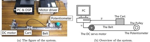
The cart on the linear rail is connected to a DC motor and a positioning sensor to a belt. The position of the cart is measured using a position sensor and the value is sent to a PC through a digital signal processor (DSP) board. The control law is defined as in Figure 1. Here, we divided the cart system into an integral part and a first-order system. In this experimental equipment, the velocity of the cart cannot be measured directly. Therefore, we calculate the used velocity differential on the DSP. We set the sampling time as $T_s=0.001$ s. The output $u_2$ from $C_2$ denotes the reference signal of the velocity of the cart. The controller of the inner loop, $C_1\left({\mathit{\rho }}_1\right)$ and that of the outer loop, $C_2\left({\mathit{\rho }}_2\right)$ are PID controllers expressed as: (35) $\begin{array}{rl}{C}_1\left({\mathit{\rho }}_1\right)& ={\rho }_1^1+{\rho }_2^1\frac{T_s}{z-1}+{\rho }_3^1\frac{10}{1+10\frac{T_s}{z-1}}\end{array}$(35) (36) $\begin{array}{rl}{C}_2\left({\mathit{\rho }}_2\right)& ={\rho }_1^2+{\rho }_2^2\frac{T_s}{z-1}+{\rho }_3^2\frac{10}{1+10\frac{T_s}{z-1}}\end{array}$(36) respectively. Here, the initial parameters are expressed as follows: (37) $\begin{array}{rl}{\mathit{\rho }}_{1\mathrm{i}\mathrm{n}\mathrm{i}}& ={\left[0.10.10\right]}^{\mathrm{\top }},\end{array}$(37) (38) $\begin{array}{rl}{\mathit{\rho }}_{2\mathrm{i}\mathrm{n}\mathrm{i}}& ={\left[1.01.00\right]}^{\mathrm{\top }}.\end{array}$(38) The reference signal denotes the step and ramp signals at a distance of $10\left[\mathrm{c}\mathrm{m}\right]$.

In this verification, there are two experiment used difference reference signal. there are (a) step signal and (b) ramp signal.

5.1. Case (a): the step signal

The specifications are expressed as: (39) $\begin{array}{rl}{T}_{d1}& =\frac{0.009516}{z-0.99},\end{array}$(39) (40) $\begin{array}{rl}{T}_{d2}& =\frac{0.000995}{z-0.999}.\end{array}$(40) The experimental result with these initial parameters are illustrated as Figures 4 and 5. In Figure 4, the cart position $\mathit{y}$ is denoted by the orange line and the desired output ${\mathit{y}}_d:=T_{d2}\mathit{r}$ is denoted by the red line. In Figure 5, the output of controller $C_2$ as the reference signal of the inner loop ${\mathit{u}}_2\left({\mathit{\rho }}_{\mathrm{i}\mathrm{n}\mathrm{i}}\right)$ is denoted by the black line, the velocity of the cart as the output of the inner loop $\mathit{w}\left({\rho }_{\mathrm{i}\mathrm{n}\mathrm{i}}\right)$ is denoted by the orange dotted line, and the desired output of the inner loop ${\mathit{w}}_d\left({\rho }_{\mathrm{i}\mathrm{n}\mathrm{i}}\right):=T_{d1}{\mathit{u}}_1\left({\mathit{\rho }}_{\mathrm{i}\mathrm{n}\mathrm{i}}\right)$ is denoted by the red line.

Figure 4. Comparison of the output of the cart positioning control. The output $y\left({\rho }_{\mathrm{i}\mathrm{n}\mathrm{i}}\right)$ as the cart position with the initial parameter ${\rho }_{\mathrm{i}\mathrm{n}\mathrm{i}}$ is denoted the orange line and the desired output $y_d$ is denoted red line. The reference signal is denoted by the black line.

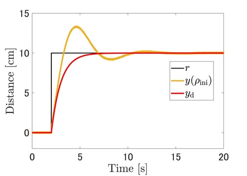
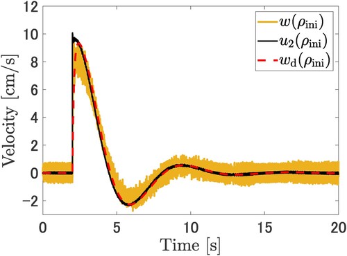
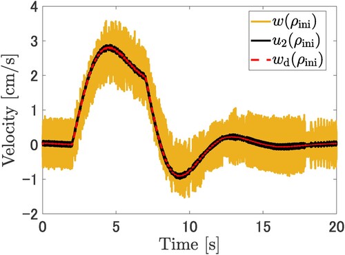
Figure 5. Comparison of the input and output signals on the inner loop. The output $w\left({\rho }_{\mathrm{i}\mathrm{n}\mathrm{i}}\right)$ of the cart speed with the initial parameter is denoted by the orange line. $u_2\left({\rho }_{\mathrm{i}\mathrm{n}\mathrm{i}}\right)$ is the reference signal for the inner loop as the reference speed. The desired speed output $w_d\left({\rho }_{\mathrm{i}\mathrm{n}\mathrm{i}}\right)$ is denoted the red dotted line made by $u_2\left({\rho }_{\mathrm{i}\mathrm{n}\mathrm{i}}\right)$.

The parameters of the controller in the cost functions are linear. Therefore, the optimal solution of each cost function can be determined using the least square method. Thus, the parameters are obtained as: (41) $\begin{array}{rl}{\mathit{\rho }}_1^{\ast }& ={[0.03680.2624-0.0020]}^{\mathrm{\top }}\end{array}$(41) (42) $\begin{array}{rl}{\mathit{\rho }}_2^{\ast }& ={\left[0.99970.00000.0007\right]}^{\mathrm{\top }}.\end{array}$(42) The results of the experiment after parameter tuning, shown in Figures 6 and 7. In Figure 6, the cart position $\mathit{y}$ is denoted by the green line and the desired output ${\mathit{y}}_d:=T_{d2}\mathit{r}$ is denoted by the red dotted line. 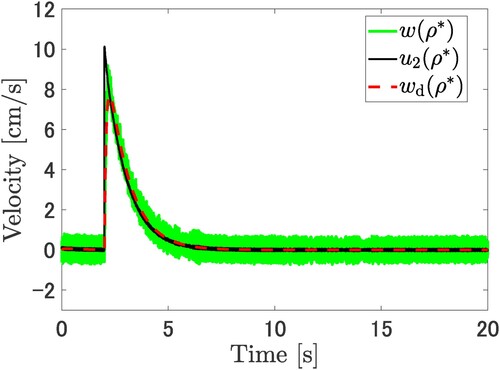In Figure 5, the output of controller $C_2$ as the reference signal of the inner loop ${\mathit{u}}_2\left({\mathit{\rho }}^{\ast }\right)$ is denoted by the black line, the velocity of the cart as the output of the inner loop $\mathit{w}\left({\rho }^{\ast }\right)$ is denoted by the green line, and the desired output of the inner loop ${\mathit{w}}_d\left({\rho }_{\mathrm{i}\mathrm{n}\mathrm{i}}\right):=T_{d1}{\mathit{u}}_1\left({\mathit{\rho }}_{\mathrm{i}\mathrm{n}\mathrm{i}}\right)$is denoted by the red dotted line.

Figure 6. Comparison of the output position of the cart system between the desired output and the output with the tuned parameter using the proposed method. The output $y\left({\rho }^{\ast }\right)$ is denoted the green line and $y_d$ is denoted the red dotted line. The output signal after tuning is in line with the desired output by the proposed method.

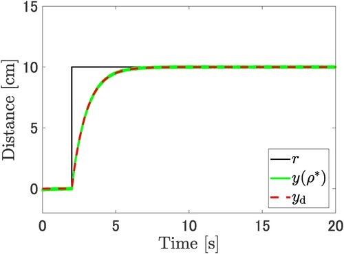
Figure 7. Comparison of the output velocity of the cart system between the desired output and the output with the tuned parameter using the proposed method. The velocity output $w\left({\rho }^{\ast }\right)$ is denoted by the green line and the desired velocity $w_d\left({\rho }^{\ast }\right)$ is denoted by the red dotted line. The velocity signal after tuning is in line with the desired velocity.

5.2. Case (b): the ramp signal

The reference signal is defined as

Moreover, the specifications are expressed as: (46) $\begin{array}{rl}{T}_{d1}& =\frac{0.09516}{z-0.9048},\end{array}$(46) (47) $\begin{array}{rl}{T}_{d2}& =\frac{0.002854z-0.002852}{z^2-1.997z+0.9971}.\end{array}$(47) Here, $T_{d2}$ is determined to achieve tracking to ramp signal. When considering the tracking to the step and ramp signals, $T_{d2}$ should be set so that $T_2$ satisfies (48) $\begin{array}{rl}& \underset{s\to 0}{lim}s(\frac{1}{s^2}-T_{d2}(s\left)\frac{1}{s^2}\right)=0,\end{array}$(48) (49) $\begin{array}{rl}& \underset{s\to 0}{lim}s{T}_{d2}\left(s\right)\frac{1}{s}=1.\end{array}$(49) This time, the adjustment parameter τ is used to set $T_{d2}$ as (50) $T_{d2}\left(s\right):=\frac{\tau s+1}{{\tau }^2{s}^2+2\tau s+1}.$(50) Equation (47(48) $\begin{array}{rl}& \underset{s\to 0}{lim}s(\frac{1}{s^2}-T_{d2}(s\left)\frac{1}{s^2}\right)=0,\end{array}$(48) ) is the discretization of Equation (50(51) $\begin{array}{rl}{\mathit{\rho }}_1^{\ast }& ={[0.04470.2565-0.0021]}^{\mathrm{\top }}\end{array}$(51) ) with zero-order hold.

The experimental result with these initial parameters are illustrated as Figures 8 and 9. In Figures 8 and 9, Notations are the same as for Figures 4 and 5.

Figure 8. Comparison of the output of the cart positioning control. The output $y\left({\rho }_{\mathrm{i}\mathrm{n}\mathrm{i}}\right)$ as the cart position with the initial parameter ${\rho }_{\mathrm{i}\mathrm{n}\mathrm{i}}$ is denoted the orange line and the desired output $y_d$ is denoted red line. The reference signal is denoted by the black line.

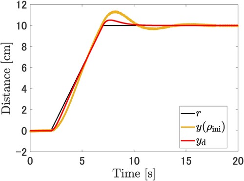
Figure 9. Comparison of the input and output signals on the inner loop. The output $w\left({\rho }_{\mathrm{i}\mathrm{n}\mathrm{i}}\right)$ of the cart speed with the initial parameter is denoted by the orange line. $u_2\left({\rho }_{\mathrm{i}\mathrm{n}\mathrm{i}}\right)$ is the reference signal for the inner loop as the reference speed. The desired speed output $w_d\left({\rho }_{\mathrm{i}\mathrm{n}\mathrm{i}}\right)$ is denoted the red dotted line made by $u_2\left({\rho }_{\mathrm{i}\mathrm{n}\mathrm{i}}\right)$.

The parameters of the controller in the aforementioned cost functions are linear. Therefore, the optimal solution can be determined using the least square method. Thus, the parameters are obtained as: (51) $\begin{array}{rl}{\mathit{\rho }}_1^{\ast }& ={[0.04470.2565-0.0021]}^{\mathrm{\top }}\end{array}$(51) (52) $\begin{array}{rl}{\mathit{\rho }}_2^{\ast }& ={[2.69602.0446-0.1045]}^{\mathrm{\top }}.\end{array}$(52) The results of the experiment after parameter tuning are shown in Figures 10 and 11. In Figures 10 and 11, Notations are the same as for Figures 6 and 7.

Figure 10. Comparison of the output position of the cart system between the desired output and the output with the tuned parameter using the proposed method. The output $y\left({\rho }^{\ast }\right)$ is denoted the green line and $y_d$ is denoted the red dotted line. The output signal after tuning is in line with the desired output by the proposed method.

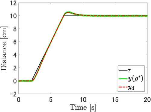
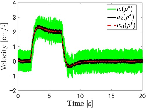
Figure 11. Comparison of the output velocity of the cart system between the desired output and the output with the tuned parameter using the proposed method. The velocity output $w\left({\rho }^{\ast }\right)$is denoted by the green line and the desired velocity $w_d\left({\rho }^{\ast }\right)$ is denoted the red dotted line. The velocity signal after tuning is in line the desired velocity.

5.3. Discussion

First, we consider the result of the outer-loop characteristic. According to Figures 6 and 10, the output signal $\mathit{y}\left({\mathit{\rho }}^{\ast }\right)$ can be tracked to the desired output ${\mathit{y}}_d$, respectively.

Next, we consider the result of the inner-loop characteristic. Here, we set the same $T_{d1}$ on both experiments, but each ${\mathit{\rho }}_2^{\ast }$ has a liitle of difference. This difference is caused by the PE condition of each output and the observation noise. According to Figures 7 and 11, although they have some difference between each ${\mathit{\rho }}^{\ast }$, the characteristics of the inner loop can achieve the desired output provided by Equation (40(40) $\begin{array}{rl}{T}_{d2}& =\frac{0.000995}{z-0.999}.\end{array}$(40) ) because the output velocity can be tracked to the desired velocity respectively.

In this verification, the differentiator parameters of the inner loop are calculated as negative. This is due to the influence of the approximate differentiator and does not affect the stability of the control system as instability or unstable zeros.

6. Conclusion

In this study, we proposed a data-driven controller design for a cascade system. Two controllers can be tuned independently in this system using two cost functions. Furthermore, the optimal solution can be easily obtained using the least square method when the parameters of the controller are linear. This is because the internal model architecture is virtually used for controller tuning. The effect of the noise and the disturbance should be theoretically studied in the future. In addition, the application of this study to the class of unstable and non-minimum phase systems is also an important research direction.

Disclosure statement

The authors declare no conflicts of interest associated with this manuscript.

Additional information

Funding

This work was supported by JSPS.

Notes on contributors

Taichi Ikezaki

Taichi Ikezaki received his B.E and M.E degrees from the University of Electro-Communications, Japan, in 2018 and 2020, respectively. Currently, He is a Ph.D. student in Graduate school of Informatics and Engineering, the University of Electro-Communications since 2020. He is currently engaged in research on data-driven control. He is a student member of the SICE and IEEJ.

Osamu Kaneko

Osamu Kaneko received his B.E. and M.E. degrees from the Nagaoka University of Technology, Japan, and Ph.D. from Osaka University, Japan, in 1992, 1994, and 2005, respectively. In 1999, he joined Osaka University as an Assistant professor. In 2009, he joined Kanazawa University as an Associate professor. In 2015, he moved to the University of Electro-Communications as a Professor His research interests include control system theory and its applications. He received the Best Paper Award from the SICE in 2012, Pioneer Technology Award of Control Division from the SICE in 2015, and so on. He is a member of the IEEE, SICE, IEEJ, ISIJ, ISCIE, and JSME.

Notes

1 Corp.ServoTechno in Japan.

References

- Morari M, Zafiriou E. Robust process control. Prentice-Hall; 1989.
- Hjalmarsson H, Gevers M, Gunnarsson S, et al. Iterative feedback tuning: theory and applications. IEEE Control Syst Mag. 1998;18(4):26–41.
- Campi MC, Lecchini A, Savaresi SM. Virtual reference feedback tuning – a direct method for the design of feedback controllers. Automatica. 2002;38(8):1337–1346.
- Souma S, Kaneko O, Fujii T. A new approach to parameter tuning of controllers by using one-shot experimental data. Trans Inst Syst Control Inf Eng. 2004;17(12):528–536.
- Ikezaki T, Kaneko O. A new approach to parameter tuning of controllers by using output data of closed loop system – virtual internal model tuning. IEEJ Trans Electron Inf Syst. 2019;39(7):780–785.
- Nguyen HQ, Kaneko O. A new prefilter approach to virtual reference feedback tuning for cascade control systems. In: Proceedings of SICE Annual Conference 2017; 2018. p. 1472–1475.
- Previdi F, Belloli D, Cologni A, et al. Virtual reference feedback tuning (VRFT) design of cascade control systems with application to an electro-hydrostatic actuator. In: 5th IFAC Symposium on Mechatronic Systems. Boston Cambridge (MA), USA: Marriott; 2010. p. 626–632.
- Nguyen HT, Kaneko O. Fictitious reference iterative tuning for cascade PI controllers of DC motor speed control system. IEEJ Trans Electron Inf Syst. 2016;139(5):710–714.