Jaccard matrix for nonlinear filter statistics

ABSTRACT

We propose the Jaccard matrix (JM) and the Jaccard cell (JC), define them as the extended concepts of the Jaccard index, and theoretically and numerically analyze them. The data on the Euclidean plane can derive the JM as a sparse matrix. We show the JC inherits the feature of similarity of the Jaccard index as the exponential function of mutual information. We theoretically and numerically confirm that the local correlation coefficient of the data on the Euclidean plane relates the JC to the mutual information. Although one could potentially select an arbitrary cell size of the grid to make the JM, the knowledge we can obtain from the matrix decreases if the cell size is too big or too small to distinguish the data clusters appropriately. Therefore, the JM needs a computational procedure to determine the cell size within the appropriate scale. Maximizing the variance of the JCs supports determining the unique cell size, which value locates in the middle range of the parabolic function of the cell-size parameter. The JM could derive an index extracting nonlinear correlation of the data. The maximized standard deviation of the JCs as such an index is a decreasing function of the noise scale of the data under the constraint conditions. The ability to determine the homogeneous rectangular grid pattern of the JM might be a significant feature for finding nonlinear correlation. We would summarize this study as that of a nonlinear filter working as an efficient component of explainable AI and statistics.

KEYWORDS:

• Jaccard index
• nonlinear correlation
• sparse matrix
• mutual information
• data mining
• variance maximization

1. Introduction

Discovering functionality between two variables is a significant task of data mining. Pearson correlation coefficient (PCC) [1], a measure of linearity between two variables, is a classical tool for the task, but it cannot detect a general association, such as a nonlinear function with random noise. Such an association not to be measured adequately by PCC is called nonlinear correlation [2]. The maximum information coefficient (MIC) is a measure proposed by Reshef et al. [3] of the nonlinear correlation between two variables. MIC is the maximum value of mutual information (MI) calculated for the divided two-dimensional spaces into various grid patterns. As the recent studies on MIC, for instance, there is a new algorithm to optimize it [4] and is an extension to apply to multi-dimensional data [5]. MIC is one of the excellent practices in advanced applications of MI as a well-known measure. We are interested in developing a method to create an index of nonlinear correlation by aggregating a canonical measure modified appropriately, inspired by the procedure of MIC.

On the other hand, as the context from a general view of mathematical formulation, we pay attention to mathematical operability and analyzability. A general association of data of two variables, including nonlinear correlation, can be regarded as a binary relation R defined as a subset of a direct product $A\times B$ of data sets A and B. A function is a binary relation such that any element of A is in a relation with one and only one element of B. In this sense, data mining for two variables implies knowledge discovery of binary relations or functions from observed data with random noises. The studies on machine learning to estimate such relations or functions suggest the effectivity of matrix representation in terms of operability and analyzability for the mathematical models. The rectangles of the grids of MIC are not congruent to each other, and it might have a disadvantage in terms of mathematical formulation and operation via matrix representation.

Moreover, several experimental sciences have developed indices of similarity between two sets. Jaccard index is proposed as a measure of the similarity in plant biology [6]. It has several versions coming from different disciplines, such as Tanimoto coefficient [7] in computer science, Tversky index [8] in psychology, pARIs [9–12] in cognitive science. These indices have almost the same forms defined as a quotient of dividing a meet of two sets by a join of them. Especially, pARIs based on the research of causal inference [13] including causal induction has interesting backgrounds in terms of detection of general association. Causal induction is a cognitive feature of humans finding a causality from the co-occurrence of two kinds of events [14]. In this context, the indices give non-parametric statistic models as the strength of recognizing causality. The two kinds of events of the models can be assigned to Bernoulli variables when we regard the models as functions with random variables in probability theory. pARIs is an index of the causal induction well reflecting human cognitive features, although why the index well fits human behaviour is not known. It also has the same mathematical form as the Jaccard index.

As the introduction of the present article, we gave the above overview of the three contexts, i.e. data mining of nonlinear correlation, operability and analyzability of mathematical method, and the indices of similarity of sets originated from the experimental sciences. At the junction of the above three contexts, we propose the concepts of the Jaccard cell and the Jaccard matrix. Jaccard matrix is defined as multi-dimensional Jaccard indices by one of the authors of the present article. The first idea of that appeared as pARIX in 2014 [15], and the name of the Jaccard matrix appeared in 2016 [16]. The Jaccard matrix as a component of statistical informatics let be independent of pARIs and pARIX connected to cognitive sciences in the description of this article. This concept in this article is well defined and analysed mathematically, but that in these previous studies sufficiently had been not yet. Concretely, we think that the idea of monotonicity in the previous studies was too rough to analyse the results. The mathematical improvements in this study promote an understanding of the meaning of aggregation of the Jaccard index and of the mechanism of nonlinear correlation derived from it theoretically and numerically.

In the following second section of the present article, we induce the Jaccard cell and Jaccard matrix from the Jaccard index and pARIs. In the third section, we mathematically define the Jaccard cell and Jaccard matrix for the data on the Euclidean plane and show their computational procedure. In the fourth section, we study the mathematical features of the Jaccard cell, which is approximated locally by the exponential function of MI. In the fifth section, we study a simple model of the variance of the Jaccard cells induced from the approximated equation and show that maximizing the variance of the Jaccard cells supports determining the unique cell size. In the sixth section, by the simulations, we numerically analyse the features of the Jaccard cell and Jaccard matrix theoretically shown in the previous sections. Finally, we briefly discuss the maximized standard deviation of the Jaccard cells as a decreasing function of the noise scale of the data in terms of nonlinear correlation and summarize this study as that of a nonlinear filter.

2. Jaccard cell and Jaccard matrix

In this section, we define the Jaccard cell and Jaccard matrix. Their names inherit from the Jaccard index, known as the first one of the affiliated indices. We introduce them as a generalization of a statistical index of causal induction, pARIs, which is one of such indices, The explanation might make our acceptance of their following calculation procedures easy.

2.1. pARIs and Jaccard index

In the quantitative studies of causal induction, the counting information of co-occurrence events is given by a form so-call $2\times 2$ contingency table [14]. Let C and E be events that correspond to causes and effects. Let a, b, c, d be frequency of occurrence of the events, $(C\wedge E)$, $(C\wedge \mathrm{\neg }E)$, $(\mathrm{\neg }C\wedge E)$, $(\mathrm{\neg }C\wedge \mathrm{\neg }E)$, where ¬ be the negation. Then the $2\times 2$ contingency table is given as Table 1.

Table 1. $2\times 2$ contingency table.

Effect \ Cause	C	$\mathrm{\neg }C$
E	a	c
$\mathrm{\neg }E$	b	d

Note that Table 1 is the transposed $2\times 2$ contingency table of [14]; i.e. we swap the row and column of Table 1 to be easier to associate the row and column of the table with that of the matrix and with the horizontal x-axis and vertical y-axis of ${\mathbb{R}}^2$ in the following sections. In addition, even not to distinguish rows with columns of Table 1 and the following Table 2 does not make trouble in our study, since the Jaccard cell and pARIs are symmetric to swapping rows with columns. Although pARIs is an index of causal induction, it has no asymmetricity between cause and effect.

Table 2. $n\times m$ contingency table.

	$X_0$	···	$X_j$	···	$X_{m-1}$
$Y_0$			$c_{0j}$
⋮			⋮
$Y_i$	$c_{i0}$	···	$c_{ij}$	···	$c_{im-1}$
⋮			⋮
$Y_{n-1}$			$c_{n-1j}$

Given information of the $2\times 2$ contingency table, we can define pARIs as a statistical index of causal induction [9, 11] by the following: (1) $pARIs:=\frac{a}{a+b+c},$(1) where it satisfies $0\le pARIs\le 1$ for all $a,b,c\in \mathbb{N}$. Jaccard index is defined as $N(S_A\cap S_B)/N(S_A\cup S_B)$, where $S_A$ and $S_B$ are sets, and $N\left(S\right)$ is the number of elements of the set S. pARIs (1(1) $pARIs:=\frac{a}{a+b+c},$(1) ) has the same mathematical form as the Jaccard index. For N: = a + b + c + d, we obtain the relative frequency on $C\wedge E$ and $C\vee E$, a/N and $(a+b+c)/N$. If these are replaced by occurrence probabilities $Pr(C\wedge E)$ and $Pr(C\vee E)=Pr(C\wedge E)+Pr(C\wedge \mathrm{\neg }E)+Pr(\mathrm{\neg }C\wedge E)$, then we obtain pARIs as a model of strength of human causal inference: (2) $pARIs=\frac{Pr(C\wedge E)}{Pr(C\vee E)}.$(2)

2.2. Definition of Jaccard cell and Jaccard matrix

In this section, we define the Jaccard cell and Jaccard matrix. Let X and Y be Bernoulli random variables $X,Y:\mathrm{\Omega }=\left\{\mathrm{n}\mathrm{o}\mathrm{t}\mathrm{o}\mathrm{c}\mathrm{c}\mathrm{u}\mathrm{r},\mathrm{o}\mathrm{c}\mathrm{c}\mathrm{u}\mathrm{r}\right\}\to \{0,1\}$. First, we define an index ψ as the following: (3) $\psi :=\frac{Pr\left(\right(X=1)\wedge (Y=1\left)\right)}{Pr\left(\right(X=1)\vee (Y=1\left)\right)}.$(3) Equation (3(3) $\psi :=\frac{Pr\left(\right(X=1)\wedge (Y=1\left)\right)}{Pr\left(\right(X=1)\vee (Y=1\left)\right)}.$(3) ) is the same mathematical form as the Jaccard index and pARIs. It is a model for the Jaccard index and pARIs in probability theory.

Secondly, we define Jaccard cell ${\psi }_{ij}$ as a generalization of the index ψ in (3(3) $\psi :=\frac{Pr\left(\right(X=1)\wedge (Y=1\left)\right)}{Pr\left(\right(X=1)\vee (Y=1\left)\right)}.$(3) ) to that of multi-dimensional Bernoulli random vectors. Let $\mathbf{X}=(X_0,\dots ,X_j,\dots ,X_{m-1})$ and $\mathbf{Y}=(Y_0,\dots ,Y_i,\dots ,Y_{n-1})$ be one-hot vectors following the categorical distributions, (4) $\{\begin{array}{l}{P}_{\mathrm{c}\mathrm{a}\mathrm{t}}^{\left(\mathbf{X}\right)}(k=j)=Pr(X_j=1)=p_j^{\left(\mathbf{X}\right)},\\ P_{\mathrm{c}\mathrm{a}\mathrm{t}}^{\left(\mathbf{Y}\right)}(k=i)=Pr(Y_i=1)=p_i^{\left(\mathbf{Y}\right)},\end{array}$(4) where the one-hot encoding or 1-of-K encoding, like $\mathbf{X}=(0,0,\dots ,1,\dots ,0)$, is well known in machine learning. A categorical distribution $P_{\mathrm{c}\mathrm{a}\mathrm{t}}$, also called a generalized Bernoulli distribution, is a particular case of the multi-nomial distribution [17]. Given the above $\mathbf{X}$ and $\mathbf{Y}$, we define Jaccard cell ${\psi }_{ij}$ as the following: (5) ${\psi }_{ij}:=\frac{Pr\left(\right(X_j=1)\wedge (Y_i=1\left)\right)}{Pr\left(\right(X_j=1)\vee (Y_i=1\left)\right)}.$(5) The given $X_j$ and $Y_i$ equal $X_j,Y_i:\mathrm{\Omega }=\{\mathrm{n}\mathrm{o}\mathrm{t}\mathrm{o}\mathrm{c}\mathrm{c}\mathrm{u}\mathrm{r},\mathrm{o}\mathrm{c}\mathrm{c}\mathrm{u}\mathrm{r}\}\to \{0,1\}(\mathrm{\forall }j,i\in \mathbb{N}(0\le j\le m-1,0\le i\le n-1\left)\right)$ following the Bernoulli random variables under the condition, (6) $Pr(\sum _{j=0}^{m-1}{X}_j=1)=Pr(\sum _{i=0}^{n-1}{Y}_i=1)=1.$(6) Consequently, the Jaccard cell (5(5) ${\psi }_{ij}:=\frac{Pr\left(\right(X_j=1)\wedge (Y_i=1\left)\right)}{Pr\left(\right(X_j=1)\vee (Y_i=1\left)\right)}.$(5) ) is a natural extension of the index (3(3) $\psi :=\frac{Pr\left(\right(X=1)\wedge (Y=1\left)\right)}{Pr\left(\right(X=1)\vee (Y=1\left)\right)}.$(3) ) that is equivalent to the Jaccard index and pARIs. Moreover, we define the Jaccard matrix as the following matrix: (7) $\mathrm{\Psi }:=\left({\psi }_{ij}\right),$(7) given by aggregating the Jaccard cell (5(5) ${\psi }_{ij}:=\frac{Pr\left(\right(X_j=1)\wedge (Y_i=1\left)\right)}{Pr\left(\right(X_j=1)\vee (Y_i=1\left)\right)}.$(5) ).

Let us be back to the context of pARIs. The extension to the Jaccard cell means that “the event occurs or not” is replaced by “the event indexed by i occurs.” In this sense, the $2\times 2$ contingency table as Table 1 is also extended to $n\times m$ contingency table as Table 2, where $c_{ij}\in \mathbb{N}\cup \left\{0\right\}$ is the number of data on event occurrence of $(X_j=1)\wedge (Y_i=1)$. Table 2 derives a frequency distribution on event occurrence: (8) $Pr\left(\right(X_j=1)\wedge (Y_i=1\left)\right)=c_{ij}/N_c$(8) and (9) $\begin{array}{rl}& Pr\left(\right(X_j=1)\vee (Y_i=1\left)\right)\\ & =Pr(X_j=1)+Pr(Y_i=1)\\ & -Pr\left(\right(X_j=1)\wedge (Y_i=1\left)\right)\\ & ={\frac{1}{N}}_c(\sum _{i^{\prime }=0}^{n-1}{c}_{i^{\prime }j}+\sum _{j^{\prime }=0}^{m-1}{c}_{i{j}^{\prime }}-c_{ij}),\end{array}$(9) where $N_c:=\sum _{i=0}^{n-1}\sum _{j=0}^{m-1}{c}_{ij}$ is the data size. Consequently, Equations (5(5) ${\psi }_{ij}:=\frac{Pr\left(\right(X_j=1)\wedge (Y_i=1\left)\right)}{Pr\left(\right(X_j=1)\vee (Y_i=1\left)\right)}.$(5) ), (8(8) $Pr\left(\right(X_j=1)\wedge (Y_i=1\left)\right)=c_{ij}/N_c$(8) ), and (9(9) $\begin{array}{rl}& Pr\left(\right(X_j=1)\vee (Y_i=1\left)\right)\\ & =Pr(X_j=1)+Pr(Y_i=1)\\ & -Pr\left(\right(X_j=1)\wedge (Y_i=1\left)\right)\\ & ={\frac{1}{N}}_c(\sum _{i^{\prime }=0}^{n-1}{c}_{i^{\prime }j}+\sum _{j^{\prime }=0}^{m-1}{c}_{i{j}^{\prime }}-c_{ij}),\end{array}$(9) ) derive the following Jaccard cell given statistically: (10) ${\psi }_{ij}=\frac{c_{ij}}{\sum _{j^{\prime }=0}^{m-1}{c}_{i{j}^{\prime }}+\sum _{i^{\prime }=0}^{n-1}{c}_{i^{\prime }j}-c_{ij}}.$(10) The denominator of Jaccard cell (10(10) ${\psi }_{ij}=\frac{c_{ij}}{\sum _{j^{\prime }=0}^{m-1}{c}_{i{j}^{\prime }}+\sum _{i^{\prime }=0}^{n-1}{c}_{i^{\prime }j}-c_{ij}}.$(10) ) implies the total number of the local cross-shaped region of $n\times m$ contingency table.

In this section, we defined the Jaccard cell and Jaccard matrix. $pARIX(i,j)$ of Equation (14) in [15] is mathematically equivalent to the Jaccard cell ${\psi }_{ij}$ defined in Equation  (5(5) ${\psi }_{ij}:=\frac{Pr\left(\right(X_j=1)\wedge (Y_i=1\left)\right)}{Pr\left(\right(X_j=1)\vee (Y_i=1\left)\right)}.$(5) ), except for the insignificant difference about the indices, $(i,j)$. Now, it is reasonable to construct their concept strictly and to give the starting point afresh to research this theme as mathematics for information systems away from the context of cognitive sciences, including pARIs and pARIX.

3. Jaccard matrix induced from the data on the Euclidean plane

In this section, we induce the Jaccard matrix from the data on the Euclidean plane and give the representations to compute it. See Figure 1 to understand the following definitions briefly.

Figure 1. A sketch of the two-dimensional rectangular space $S^x\times S^y\subset {\mathbb{R}}^2$ to define the Jaccard matrix and the cruciform region $S_1\cup S_2$ to calculate the Jaccard cell.

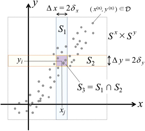
Assume a two-dimensional rectangular space $S^x\times S^y\subset {\mathbb{R}}^2$. Let us divide $S^x\times S^y$ into the grid as the direct sums of subspaces, $S^x:=\coprod _{j=0}^{m-1}{S}_j^x$ and $S^y:=\coprod _{i=0}^{n-1}{S}_i^y$, where $m,n\in \mathbb{N}$ are the number of the sections of the rows and columns. $S_j^x\times S_i^y$ expresses a small rectangular cell in the grid. $(x_0,y_0)$ and $(x_{m-1},y_{n-1})$ express the centre points of the cells at the bottom left and top right in ${\mathbb{R}}^2$. Consequently the size of each cell is $\mathrm{\Delta }x=(x_{m-1}-x_0)/(m-1)$ and $\mathrm{\Delta }y=(y_{n-1}-y_0)/(n-1)$, thus $S_j^x\times S_i^y$ is concretely expressed by $[x_j-0.5\mathrm{\Delta }x,x_j+0.5\mathrm{\Delta }x)\times [y_i-0.5\mathrm{\Delta }y,y_i+0.5\mathrm{\Delta }y)$, and the centre point is $(x_j,y_i)=(x_0+j\mathrm{\Delta }x,y_0+i\mathrm{\Delta }y)$.

Assume that data $\mathcal{D}:=\left\{\right(x^{\left(\alpha \right)},y^{\left(\alpha \right)})|\alpha =1,..,N_c\}\in S^x\times S^y$ are observed. We can calculate an index j of the range $S_j^x$ by $j=\lfloor (x^{\left(\alpha \right)}-x_{Bmin})/\mathrm{\Delta }x\rfloor$, where $x_{Bmin}:=x_0-0.5\mathrm{\Delta }x$. Since $x_{Bmin}+j\mathrm{\Delta }x\le x^{\left(\alpha \right)}<x_{Bmin}+(j+1)\mathrm{\Delta }x$, thus $j\le (x^{\left(\alpha \right)}-x_{Bmin})/\mathrm{\Delta }x<j+1$. We can also calculate $i=\lfloor (y^{\left(\alpha \right)}-y_{Bmin})/\mathrm{\Delta }y\rfloor$ for data $y^{\left(\alpha \right)}$ in the same way, where $y_{Bmin}:=y_0-0.5\mathrm{\Delta }y$.

Based on the above procedure, we count the number of the data $c_{ij}$ observed in each cell $S_j^x\times S_i^y$, which corresponds to $S_3=S_{12}$ in Figure 1. It derives a $n\times m$ matrix of non-negative integers, (11) $C:=\left(\begin{array}{ccccc}{c}_{00}& \cdots & c_{0j}& \cdots & c_{1,m-1}\\ ⋮& & ⋮& & ⋮\\ c_{i0}& \cdots & c_{ij}& \cdots & c_{i,m-1}\\ ⋮& & ⋮& & ⋮\\ c_{n-1,0}& \cdots & c_{n-1,j}& \cdots & c_{n-1,m-1}\end{array}\right),$(11) which corresponds to a $n\times m$ contingency table.

Let us adjust some matrix representations for GPU programming. Defining ${\mathbf{1}}_n$ by a n-dimensional column vector that has 1 as all of the elements, i.e. ${\mathbf{1}}_n:={}^t(1,\dots ,1)$, we obtain the relationship between the matrix C and the data size $N_c$ as the following: (12) ${}^t{\mathbf{1}}_{n}C{\mathbf{1}}_m=\sum _{i=0}^{n-1}\sum _{j=0}^{m-1}{c}_{ij}=N_c.$(12) On the other hand, defining ${\mathbf{1}}_{n\times m}$ by the $n\times m$ matrix that has 1 as all of the elements, i.e. ${\mathbf{1}}_{n\times m}:={\mathbf{1}}_n{}^t{\mathbf{1}}_m$, we obtain the following $n\times m$ matrix H: (13) $\begin{array}{rl}H& :=C{\mathbf{1}}_m{}^t{\mathbf{1}}_m+{\mathbf{1}}_n{}^t{\mathbf{1}}_{n}C-C\\ & =C{\mathbf{1}}_{m\times m}+{\mathbf{1}}_{n\times n}C-C.\end{array}$(13) The element of H, $h_{ij}$, is the denominator of the Jaccard cell ${\psi }_{ij}$, as well as $c_{ij}$ is the numerator of it, since Equation (13(13) $\begin{array}{rl}H& :=C{\mathbf{1}}_m{}^t{\mathbf{1}}_m+{\mathbf{1}}_n{}^t{\mathbf{1}}_{n}C-C\\ & =C{\mathbf{1}}_{m\times m}+{\mathbf{1}}_{n\times n}C-C.\end{array}$(13) ) derives (14) $h_{ij}=\sum _{j^{\prime }=0}^{m-1}{c}_{i{j}^{\prime }}+\sum _{i^{\prime }=0}^{n-1}{c}_{i^{\prime }j}-c_{ij}.$(14) The region to count these data corresponds to the cruciform one of $S_1\cup S_2$ in Figure 1. Equation (14(14) $h_{ij}=\sum _{j^{\prime }=0}^{m-1}{c}_{i{j}^{\prime }}+\sum _{i^{\prime }=0}^{n-1}{c}_{i^{\prime }j}-c_{ij}.$(14) ) has the other representation, i.e. (15) $h_{ij}=\sum _{j^{\prime }\ne j}{c}_{i{j}^{\prime }}+\sum _{i^{\prime }\ne i}{c}_{i^{\prime }j}+c_{ij}.$(15) For all i, j, $c_{ij}\ge 0$ thus $\sum _{j^{\prime }\ne j}{c}_{i{j}^{\prime }}+\sum _{i^{\prime }\ne i}{c}_{i^{\prime }j}\ge 0$. Therefore, $h_{ij}=0\Rightarrow c_{ij}=0\mathrm{f}\mathrm{o}\mathrm{r}\mathrm{a}\mathrm{l}\mathrm{l}i,j$. Consequently, $n\times m$ Jaccard matrix Ψ is given by an element-wise quotient of the matrices C and H as the following: (16) $\mathrm{\Psi }=C\oslash H:=(c_{ij}\oslash h_{ij})=\left({\psi }_{ij}\right),$(16) where (17) ${\psi }_{ij}:=c_{ij}\oslash h_{ij}:=\{\begin{array}{cc}{c}_{ij}/h_{ij}& (h_{ij}\ne 0),\\ 0& (h_{ij}=0).\end{array}$(17) The mean of ${\psi }_{ij}$, $\overline{\psi }$, is calculated by (18) $\overline{\psi }:=\frac{1}{N_c}\sum _{i=0}^{n-1}\sum _{j=0}^{m-1}{\psi }_{ij}=\frac{{}^t{\mathbf{1}}_n\mathrm{\Psi }{\mathbf{1}}_m}{{}^t{\mathbf{1}}_{n}C{\mathbf{1}}_m}.$(18) The variance of ${\psi }_{ij}$, $V_{\psi }$, is calculated by (19) $\begin{array}{rl}{V}_{\psi }& :=\frac{1}{N_c}\sum _{i=0}^{n-1}\sum _{j=0}^{m-1}{\psi }_{ij}^2-(\overline{\psi }{)}^2\\ & =\frac{{}^t{\mathbf{1}}_n(\mathrm{\Psi }\circ \mathrm{\Psi }){\mathbf{1}}_m}{{}^t{\mathbf{1}}_{n}C{\mathbf{1}}_m}-{\left(\frac{{}^t{\mathbf{1}}_n\mathrm{\Psi }{\mathbf{1}}_m}{{}^t{\mathbf{1}}_{n}C{\mathbf{1}}_m}\right)}^2,\end{array}$(19) where ° is Hadamard product or element-wise product defined by $A\circ B:=\left(a_{ij}{b}_{ij}\right)$.

For instance, of the concrete values of the above, we can calculate the following example: assume $S^x\times S^y:=[0,2]\times [0,3]$ and $\mathrm{\Delta }x=\mathrm{\Delta }y=1$, then we obtain six cells of the grid in the space. If observed data are given as

$\mathcal{D}=\left\{\right(0.5,0.7),(0.3,0.2),(0.4,2.1),(1.6,2.5),(1.1,1.5),(1.3,1.7),(1.8,1.2\left)\right\}$, they derive the following matrix: (20) $C=\left(\begin{array}{cc}{c}_{00}& c_{01}\\ c_{10}& c_{11}\\ c_{20}& c_{21}\end{array}\right)=\left(\begin{array}{cc}2& 0\\ 0& 3\\ 1& 1\end{array}\right),$(20) then $N_c=7$, and then $c_{11}=3$ means that we observed three data in the grid, $[1,2]\times [1,2]$. For the matrix C, we obtain the matrix H and the Jaccard matrix Ψ as the following: (21) $H=\left(\begin{array}{cc}3& 0\\ 0& 4\\ 4& 5\end{array}\right),\mathrm{\Psi }=\left(\begin{array}{cc}2/3& 0\\ 0& 3/4\\ 1/4& 1/5\end{array}\right).$(21) It is not rare that the matrix C is sparse. The above procedure is inefficient when C is a sparse matrix, although it helps the programming of GPU computing for them. Indeed, the data based on an ordinary function $f:S^x\subset \mathbb{R}\to \mathbb{R}$ can derive a sparse matrix C by sufficiently small $\mathrm{\Delta }x$. Therefore, we can use the list including only the non-zero elements of C, such as the format of COO or CSR [18, 19], for effective programming. For instance, the COO format of the matrix (20(20) $C=\left(\begin{array}{cc}{c}_{00}& c_{01}\\ c_{10}& c_{11}\\ c_{20}& c_{21}\end{array}\right)=\left(\begin{array}{cc}2& 0\\ 0& 3\\ 1& 1\end{array}\right),$(20) ) is given as the following: (22) $\begin{array}{rl}{C}_{\mathrm{C}\mathrm{O}\mathrm{O}}& =\left[\begin{array}{c}\left[\mathrm{t}\mathrm{h}\mathrm{e}\mathrm{l}\mathrm{i}\mathrm{s}\mathrm{t}\mathrm{o}\mathrm{f}\mathrm{t}\mathrm{h}\mathrm{e}\mathrm{n}\mathrm{o}\mathrm{n}-\mathrm{z}\mathrm{e}\mathrm{r}\mathrm{o}{c}_{ij}\right]\\ \left[\mathrm{t}\mathrm{h}\mathrm{e}\mathrm{l}\mathrm{i}\mathrm{s}\mathrm{t}\mathrm{o}\mathrm{f}\mathrm{t}\mathrm{h}\mathrm{e}\mathrm{r}\mathrm{o}\mathrm{w}\mathrm{i}\mathrm{n}\mathrm{d}\mathrm{i}\mathrm{c}\mathrm{e}\mathrm{s}i\right]\\ \left[\mathrm{t}\mathrm{h}\mathrm{e}\mathrm{l}\mathrm{i}\mathrm{s}\mathrm{t}\mathrm{o}\mathrm{f}\mathrm{t}\mathrm{h}\mathrm{e}\mathrm{c}\mathrm{o}\mathrm{l}\mathrm{u}\mathrm{m}\mathrm{n}\mathrm{i}\mathrm{n}\mathrm{d}\mathrm{i}\mathrm{c}\mathrm{e}\mathrm{s}j\right]\end{array}\right]\\ & =\left[\begin{array}{c}[2,3,1,1]\\ [0,1,2,2]\\ [0,1,0,1]\end{array}\right].\end{array}$(22)

4. Mathematical analyses of the Jaccard cell and Jaccard matrix

In this section, we analyse the mathematical features of the Jaccard cell derived from data on $S^x\times S^y\subset {\mathbb{R}}^2$.

4.1. Jaccard cell depending on the cell-size parameters

The value of the Jaccard cell depends on the size of the cell $(\mathrm{\Delta }x,\mathrm{\Delta }y)$. Therefore, we construct a representation of the Jaccard cell explicitly integrated with cell-size parameters, i.e. we replace the number of the data discretely counted in Equation (10(10) ${\psi }_{ij}=\frac{c_{ij}}{\sum _{j^{\prime }=0}^{m-1}{c}_{i{j}^{\prime }}+\sum _{i^{\prime }=0}^{n-1}{c}_{i^{\prime }j}-c_{ij}}.$(10) ) by the probability density function of them continuously integrated as the following: (23) $\begin{array}{rl}{P}_1\left(x\right)& :=Pr(x-{\delta }_x\le X<x+{\delta }_x)\\ & ={\int }_{x-{\delta }_x}^{x+{\delta }_x}{\int }_{-\mathrm{\infty }}^{\mathrm{\infty }}p(x,y)\mathrm{d}x\mathrm{d}y={\int }_{x-{\delta }_x}^{x+{\delta }_x}p\left(x\right)\mathrm{d}x,\end{array}$(23) (24) $\begin{array}{rl}{P}_2\left(y\right)& :=Pr(y-{\delta }_y\le Y<y+{\delta }_y)\\ & ={\int }_{-\mathrm{\infty }}^{\mathrm{\infty }}{\int }_{y-{\delta }_y}^{y+{\delta }_y}p(x,y)\mathrm{d}x\mathrm{d}y={\int }_{y-{\delta }_y}^{y+{\delta }_y}p\left(y\right)\mathrm{d}y,\end{array}$(24) (25) $\begin{array}{rl}{P}_3(x,y)& :=Pr(x-{\delta }_x\le X<x+{\delta }_x,\\ & y-{\delta }_y\le Y<y+{\delta }_y)\\ & ={\int }_{x-{\delta }_x}^{x+{\delta }_x}{\int }_{y-{\delta }_y}^{y+{\delta }_y}p(x,y)\mathrm{d}x\mathrm{d}y,\end{array}$(25) where ${\delta }_x,{\delta }_y>0$ are the cell-size parameters, and $p(x,y)$ is the probability density function of data observed in the point $(x,y)$. Let us write the regions of the integrals $P_1$,$P_2$, and $P_3$ as $S_1$,$S_2$, and $S_3$. $P_3$ means the probability of data observed in $S_3$. Figure 1 represents the regions $S_1,S_2,S_3\subset S_x\times S_y\subset {\mathbb{R}}^2$. $S_1\cup S_2$ is a local cruciform region, and $S_3=S_1\cap S_2$ is the rectangular region of the centre of the former. Using Equations (23(23) $\begin{array}{rl}{P}_1\left(x\right)& :=Pr(x-{\delta }_x\le X<x+{\delta }_x)\\ & ={\int }_{x-{\delta }_x}^{x+{\delta }_x}{\int }_{-\mathrm{\infty }}^{\mathrm{\infty }}p(x,y)\mathrm{d}x\mathrm{d}y={\int }_{x-{\delta }_x}^{x+{\delta }_x}p\left(x\right)\mathrm{d}x,\end{array}$(23) )–(25(25) $\begin{array}{rl}{P}_3(x,y)& :=Pr(x-{\delta }_x\le X<x+{\delta }_x,\\ & y-{\delta }_y\le Y<y+{\delta }_y)\\ & ={\int }_{x-{\delta }_x}^{x+{\delta }_x}{\int }_{y-{\delta }_y}^{y+{\delta }_y}p(x,y)\mathrm{d}x\mathrm{d}y,\end{array}$(25) ) and replacing the sum on $i,j\in \mathbb{N}$ with the integral on $x,y\in \mathbb{R}$, we obtain the Jaccard cell depending on the continuous variables $(x,y)$ and the cell-size parameters $({\delta }_x,{\delta }_y)$, (26) $\begin{array}{rl}\psi (x,y;{\delta }_x,{\delta }_y)& =\frac{P_3}{P_1+P_2-P_3}\\ & =\frac{{\int }_{S_1\cap S_2}p(x,y)\mathrm{d}x\mathrm{d}y}{{\int }_{S_1\cup S_2}p(x,y)\mathrm{d}x\mathrm{d}y}.\end{array}$(26) Since $S_3=(S_1\cap S_2)\subset (S_1\cup S_2)$, thus generally (27) $0\le \psi (x,y;{\delta }_x,{\delta }_y)\le 1\mathrm{f}\mathrm{o}\mathrm{r}\mathrm{a}\mathrm{l}\mathrm{l}x,y,{\delta }_x,{\delta }_y\in \mathbb{R},$(27) as well as pARIs and the Jaccard cell ${\psi }_{ij}$ in (10(10) ${\psi }_{ij}=\frac{c_{ij}}{\sum _{j^{\prime }=0}^{m-1}{c}_{i{j}^{\prime }}+\sum _{i^{\prime }=0}^{n-1}{c}_{i^{\prime }j}-c_{ij}}.$(10) ). If we divide $S^x\times S^y\subset {\mathbb{R}}^2$ into $n\times m$ rectangular cells by the procedure of the previous section, then (28) ${\psi }_{ij}=\psi (x_j,y_i;{\delta }_x,{\delta }_y),{\delta }_x=0.5\mathrm{\Delta }x,{\delta }_y=0.5\mathrm{\Delta }y,$(28) for Equations (10(10) ${\psi }_{ij}=\frac{c_{ij}}{\sum _{j^{\prime }=0}^{m-1}{c}_{i{j}^{\prime }}+\sum _{i^{\prime }=0}^{n-1}{c}_{i^{\prime }j}-c_{ij}}.$(10) ) and (26(26) $\begin{array}{rl}\psi (x,y;{\delta }_x,{\delta }_y)& =\frac{P_3}{P_1+P_2-P_3}\\ & =\frac{{\int }_{S_1\cap S_2}p(x,y)\mathrm{d}x\mathrm{d}y}{{\int }_{S_1\cup S_2}p(x,y)\mathrm{d}x\mathrm{d}y}.\end{array}$(26) ).

4.2. Jaccard cell approximated by the exponential function of MI

Correlation coefficient and MI are well-known measures for an association between two random variables. In this section, we study the mathematical relationship between the Jaccard cell (26(26) $\begin{array}{rl}\psi (x,y;{\delta }_x,{\delta }_y)& =\frac{P_3}{P_1+P_2-P_3}\\ & =\frac{{\int }_{S_1\cap S_2}p(x,y)\mathrm{d}x\mathrm{d}y}{{\int }_{S_1\cup S_2}p(x,y)\mathrm{d}x\mathrm{d}y}.\end{array}$(26) ) and these measures.

Let X and Y be the random variables following the two-dimensional normal distribution $p(x,y)$ with correlation coefficient ρ as the parameter of it: (29) $\begin{array}{rl}p(x,y)& =\frac{1}{2\pi {\sigma }_x{\sigma }_y\sqrt{1-{\rho }^2}}\exp \{-\frac{1}{2(1-{\rho }^2)}\\ & \times [\frac{(x-{\mu }_x{)}^2}{{\sigma }_x^2}-2\rho \frac{(x-{\mu }_x)(y-{\mu }_y)}{{\sigma }_x{\sigma }_y}\\ & +\frac{(y-{\mu }_y{)}^2}{{\sigma }_y^2}]\}.\end{array}$(29) Assume that the observed data for the Jaccard cell (26(26) $\begin{array}{rl}\psi (x,y;{\delta }_x,{\delta }_y)& =\frac{P_3}{P_1+P_2-P_3}\\ & =\frac{{\int }_{S_1\cap S_2}p(x,y)\mathrm{d}x\mathrm{d}y}{{\int }_{S_1\cup S_2}p(x,y)\mathrm{d}x\mathrm{d}y}.\end{array}$(26) ) follows the distribution (29(29) $\begin{array}{rl}p(x,y)& =\frac{1}{2\pi {\sigma }_x{\sigma }_y\sqrt{1-{\rho }^2}}\exp \{-\frac{1}{2(1-{\rho }^2)}\\ & \times [\frac{(x-{\mu }_x{)}^2}{{\sigma }_x^2}-2\rho \frac{(x-{\mu }_x)(y-{\mu }_y)}{{\sigma }_x{\sigma }_y}\\ & +\frac{(y-{\mu }_y{)}^2}{{\sigma }_y^2}]\}.\end{array}$(29) ) in the local cell $S_3$, and the centre of the local cell is located on the expected values $({\mu }_x,{\mu }_y)$. This assumption probabilistically expresses observed data have a linear functional structure around the local space where the Jaccard cell is defined, although the spatial pattern of the data might be nonlinear globally. The strength of the linear functional structure corresponds to the correlation coefficient, and the data are normally distributed around the linear function. By the calculation in Appendix, we obtain the approximated Jaccard cell as the following: (30) $\begin{array}{rl}\psi ({\mu }_x,{\mu }_y;{\delta }_x,{\delta }_y)& =\frac{P_3({\mu }_x,{\mu }_y)}{P_1\left({\mu }_x\right)+P_2\left({\mu }_y\right)-P_3({\mu }_x,{\mu }_y)}\\ & \approx \frac{{\delta }_x{\delta }_y}{({\delta }_x{\sigma }_y+{\delta }_y{\sigma }_x)\sqrt{\frac{\pi }{2}(1-{\rho }^2)}-{\delta }_x{\delta }_y}.\end{array}$(30) In the following two cases under different conditions, we show that the Jaccard cells are locally approximated by the exponential of MI.

Case 1: the condition of the cell-size parameters that are proportional to the standard deviations of the data distribution

Let us set a sufficiently small value of δ as (31) $0<\delta \ll 1,$(31) and set the cell-size parameters, ${\delta }_x$ and ${\delta }_y$, as (32) ${\delta }_x=\delta {\sigma }_x\ll {\sigma }_x\mathrm{a}\mathrm{n}\mathrm{d}{\delta }_y=\delta {\sigma }_y\ll {\sigma }_y.$(32) Substituting the above conditions for Equation (30(30) $\begin{array}{rl}\psi ({\mu }_x,{\mu }_y;{\delta }_x,{\delta }_y)& =\frac{P_3({\mu }_x,{\mu }_y)}{P_1\left({\mu }_x\right)+P_2\left({\mu }_y\right)-P_3({\mu }_x,{\mu }_y)}\\ & \approx \frac{{\delta }_x{\delta }_y}{({\delta }_x{\sigma }_y+{\delta }_y{\sigma }_x)\sqrt{\frac{\pi }{2}(1-{\rho }^2)}-{\delta }_x{\delta }_y}.\end{array}$(30) ), we obtain the value of the approximated Jaccard cell (AJC) as the following: (33) $\left(\mathrm{A}\mathrm{J}\mathrm{C}\right):\psi ({\mu }_x,{\mu }_y;\delta ,\delta )\approx \frac{\delta }{\sqrt{2\pi (1-{\rho }^2)}-\delta }.$(33) A MI $I(X,Y)$ of two normal random variables X and Y following (29(29) $\begin{array}{rl}p(x,y)& =\frac{1}{2\pi {\sigma }_x{\sigma }_y\sqrt{1-{\rho }^2}}\exp \{-\frac{1}{2(1-{\rho }^2)}\\ & \times [\frac{(x-{\mu }_x{)}^2}{{\sigma }_x^2}-2\rho \frac{(x-{\mu }_x)(y-{\mu }_y)}{{\sigma }_x{\sigma }_y}\\ & +\frac{(y-{\mu }_y{)}^2}{{\sigma }_y^2}]\}.\end{array}$(29) ) generally depends on only the correlation coefficient ρ of them; i.e. (34) $I(X,Y)=-\frac{1}{2}\ln (1-{\rho }^2)=\ln \frac{1}{\sqrt{1-{\rho }^2}}.$(34) Therefore, if δ is sufficiently small as $\delta \ll \sqrt{2\pi (1-{\rho }^2)}$, then we obtain the value of the approximated Jaccard cell using the mutual information (JCMI) as the following: (35) $\begin{array}{rl}& \left(\mathrm{J}\mathrm{C}\mathrm{M}\mathrm{I}\right):\psi ({\mu }_x,{\mu }_y;\delta ,\delta )\approx \frac{\delta }{\sqrt{2\pi (1-{\rho }^2)}}\\ & =\frac{\delta }{\sqrt{2\pi }}{\mathrm{e}}^{I(X,Y)}.\end{array}$(35) We compare the value of (33(33) $\left(\mathrm{A}\mathrm{J}\mathrm{C}\right):\psi ({\mu }_x,{\mu }_y;\delta ,\delta )\approx \frac{\delta }{\sqrt{2\pi (1-{\rho }^2)}-\delta }.$(33) ) with that of (35(35) $\begin{array}{rl}& \left(\mathrm{J}\mathrm{C}\mathrm{M}\mathrm{I}\right):\psi ({\mu }_x,{\mu }_y;\delta ,\delta )\approx \frac{\delta }{\sqrt{2\pi (1-{\rho }^2)}}\\ & =\frac{\delta }{\sqrt{2\pi }}{\mathrm{e}}^{I(X,Y)}.\end{array}$(35) ) numerically in Section 6.1.

Studying the mathematical features of the Jaccard cell based on the approximated equations, we should pay attention to the intrinsic constraint conditions of the parameters, δ and ρ. The Jaccard cell (26(26) $\begin{array}{rl}\psi (x,y;{\delta }_x,{\delta }_y)& =\frac{P_3}{P_1+P_2-P_3}\\ & =\frac{{\int }_{S_1\cap S_2}p(x,y)\mathrm{d}x\mathrm{d}y}{{\int }_{S_1\cup S_2}p(x,y)\mathrm{d}x\mathrm{d}y}.\end{array}$(26) ) satisfies the condition (27(27) $0\le \psi (x,y;{\delta }_x,{\delta }_y)\le 1\mathrm{f}\mathrm{o}\mathrm{r}\mathrm{a}\mathrm{l}\mathrm{l}x,y,{\delta }_x,{\delta }_y\in \mathbb{R},$(27) ) exactly, therefore we generally obtain (36) $0\le P_3\le P_1+P_2-P_3\le P_1+P_2.$(36) Substituting Equations (A5(A5) $P_1\left({\mu }_x\right)={\int }_{{\mu }_x-{\delta }_x}^{{\mu }_x+{\delta }_x}p\left(x\right)\mathrm{d}x\approx 2{\delta }_x\cdot p({\mu }_x\pm {\delta }_x)=\frac{{\delta }_x}{{\sigma }_x}\sqrt{\frac{2}{\pi }}.$(A5) ), (A6(A6) $P_2\left({\mu }_y\right)={\int }_{{\mu }_y-{\delta }_y}^{{\mu }_y+{\delta }_y}p\left(y\right)\mathrm{d}y\approx 2{\delta }_y\cdot p({\mu }_y\pm {\delta }_y)=\frac{{\delta }_y}{{\sigma }_y}\sqrt{\frac{2}{\pi }}.$(A6) ), (A8(A8) $\begin{array}{rl}{P}_3({\mu }_x,{\mu }_y)& ={\int }_{{\mu }_x-{\delta }_x}^{{\mu }_x+{\delta }_x}{\int }_{{\mu }_y-{\delta }_y}^{{\mu }_y+{\delta }_y}p(x,y)\mathrm{d}x\mathrm{d}y\\ & \approx \left(2{\delta }_x\right)\cdot \left(2{\delta }_y\right)\cdot p({\mu }_x\pm {\delta }_x,{\mu }_y\pm {\delta }_y)\\ & =\frac{2{\delta }_x{\delta }_y}{\pi {\sigma }_x{\sigma }_y\sqrt{1-{\rho }^2}}.\end{array}$(A8) ) in Appendix and the conditions (31(31) $0<\delta \ll 1,$(31) ) and (32(32) ${\delta }_x=\delta {\sigma }_x\ll {\sigma }_x\mathrm{a}\mathrm{n}\mathrm{d}{\delta }_y=\delta {\sigma }_y\ll {\sigma }_y.$(32) ) for inequation (36(36) $0\le P_3\le P_1+P_2-P_3\le P_1+P_2.$(36) ), we obtain (37) $0<\frac{2{\delta }^2}{\pi \sqrt{1-{\rho }^2}}\le \frac{2\delta \sqrt{\frac{2}{\pi }(1-{\rho }^2)}-\frac{2}{\pi }{\delta }^2}{\sqrt{1-{\rho }^2}}\le 2\delta \sqrt{\frac{2}{\pi }},$(37) and then, since $|\rho |\le 1$, (38) $0<\delta \le \sqrt{\frac{\pi }{2}(1-{\rho }^2)}\le \sqrt{\frac{\pi }{2}}.$(38)

Case 2: the condition of the two cell-size parameters that have the same small value

If we set the cell-size parameters, ${\delta }_x$ and ${\delta }_y$, as the same small value (39) ${\delta }_0={\delta }_x={\delta }_y,$(39) then, by the calculation of the Appendix, we obtain the approximated value of the Jaccard cell (26(26) $\begin{array}{rl}\psi (x,y;{\delta }_x,{\delta }_y)& =\frac{P_3}{P_1+P_2-P_3}\\ & =\frac{{\int }_{S_1\cap S_2}p(x,y)\mathrm{d}x\mathrm{d}y}{{\int }_{S_1\cup S_2}p(x,y)\mathrm{d}x\mathrm{d}y}.\end{array}$(26) ) as the following: (40) $\psi ({\mu }_x,{\mu }_y;{\delta }_0,{\delta }_0)\approx \frac{{\delta }_0}{({\sigma }_x+{\sigma }_y)\sqrt{\frac{\pi }{2}(1-{\rho }^2)}-{\delta }_0}.$(40) Assuming ${\delta }_0\ll ({\sigma }_x+{\sigma }_y)\sqrt{\frac{\pi }{2}(1-{\rho }^2)}$ (i.e. $\frac{{\delta }_0}{{\sigma }_x+{\sigma }_y}\ll \sqrt{\frac{\pi }{2}(1-{\rho }^2)}\le \sqrt{\frac{\pi }{2}}$), we obtain (41) $\begin{array}{rl}\psi ({\mu }_x,{\mu }_y;{\delta }_0,{\delta }_0)& \approx \frac{{\delta }_0}{({\sigma }_x+{\sigma }_y)\sqrt{\frac{\pi }{2}(1-{\rho }^2)}}\\ & =\frac{{\delta }_0}{{\sigma }_x+{\sigma }_y}\sqrt{\frac{2}{\pi }}{\mathrm{e}}^{I(X,Y)}.\end{array}$(41) Equation (41(41) $\begin{array}{rl}\psi ({\mu }_x,{\mu }_y;{\delta }_0,{\delta }_0)& \approx \frac{{\delta }_0}{({\sigma }_x+{\sigma }_y)\sqrt{\frac{\pi }{2}(1-{\rho }^2)}}\\ & =\frac{{\delta }_0}{{\sigma }_x+{\sigma }_y}\sqrt{\frac{2}{\pi }}{\mathrm{e}}^{I(X,Y)}.\end{array}$(41) ) derives Equation (35(35) $\begin{array}{rl}& \left(\mathrm{J}\mathrm{C}\mathrm{M}\mathrm{I}\right):\psi ({\mu }_x,{\mu }_y;\delta ,\delta )\approx \frac{\delta }{\sqrt{2\pi (1-{\rho }^2)}}\\ & =\frac{\delta }{\sqrt{2\pi }}{\mathrm{e}}^{I(X,Y)}.\end{array}$(35) ) under the condition ${\delta }_0=\delta {\sigma }_x=\delta {\sigma }_y$. We analyse a simple model of the above approximated Jaccard cell (40(40) $\psi ({\mu }_x,{\mu }_y;{\delta }_0,{\delta }_0)\approx \frac{{\delta }_0}{({\sigma }_x+{\sigma }_y)\sqrt{\frac{\pi }{2}(1-{\rho }^2)}-{\delta }_0}.$(40) ) in the following section.

5. A simple model of the approximated Jaccard cells and the cell-size parameter determined uniquely

In this section, we study a simple model of the variance of the Jaccard cells (19(19) $\begin{array}{rl}{V}_{\psi }& :=\frac{1}{N_c}\sum _{i=0}^{n-1}\sum _{j=0}^{m-1}{\psi }_{ij}^2-(\overline{\psi }{)}^2\\ & =\frac{{}^t{\mathbf{1}}_n(\mathrm{\Psi }\circ \mathrm{\Psi }){\mathbf{1}}_m}{{}^t{\mathbf{1}}_{n}C{\mathbf{1}}_m}-{\left(\frac{{}^t{\mathbf{1}}_n\mathrm{\Psi }{\mathbf{1}}_m}{{}^t{\mathbf{1}}_{n}C{\mathbf{1}}_m}\right)}^2,\end{array}$(19) ) induced from the approximated Equation (40(40) $\psi ({\mu }_x,{\mu }_y;{\delta }_0,{\delta }_0)\approx \frac{{\delta }_0}{({\sigma }_x+{\sigma }_y)\sqrt{\frac{\pi }{2}(1-{\rho }^2)}-{\delta }_0}.$(40) ). As we know in the previous section, the Jaccard cell and Jaccard matrix depend on the cell-size parameters. We select the value of the cell-size parameter derived by a computable procedure to determine the Jaccard matrix uniquely. The analysis of the model in this section supports the unique determination of the Jaccard matrix and its cell-size parameter.

5.1. A simple model of the Jaccard cell

Let $\text{β}=\text{β}\left(\sigma \right)$ be a function of σ that is a standard deviation as a scale of the noise of observed data. For instance, in Equation (40(40) $\psi ({\mu }_x,{\mu }_y;{\delta }_0,{\delta }_0)\approx \frac{{\delta }_0}{({\sigma }_x+{\sigma }_y)\sqrt{\frac{\pi }{2}(1-{\rho }^2)}-{\delta }_0}.$(40) ), (42) $\text{β}=({\sigma }_x+{\sigma }_y)\sqrt{\frac{\pi }{2}(1-{\rho }^2)},$(42) which is a part of the denominator of that. 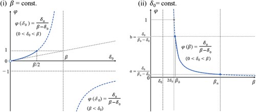In this view, we study the following equation as a model of the Jaccard cell (40(40) $\psi ({\mu }_x,{\mu }_y;{\delta }_0,{\delta }_0)\approx \frac{{\delta }_0}{({\sigma }_x+{\sigma }_y)\sqrt{\frac{\pi }{2}(1-{\rho }^2)}-{\delta }_0}.$(40) ): (43) $\phi =\frac{{\delta }_0}{\text{β}-{\delta }_0}(0<{\delta }_0\le \text{β}/2).$(43) The solid lines of (i) and (ii) in Figure 2 show sketches of the graphs of (43(43) $\phi =\frac{{\delta }_0}{\text{β}-{\delta }_0}(0<{\delta }_0\le \text{β}/2).$(43) ) in the cases that β or ${\delta }_0$ is fixed as each constant value.

Figure 2. The solid lines of (i) and (ii) show sketches of the graphs of the simple model of the Jaccard cell, Equation (43(43) $\phi =\frac{{\delta }_0}{\text{β}-{\delta }_0}(0<{\delta }_0\le \text{β}/2).$(43) ), in the cases where β or ${\delta }_0$ is fixed as each constant value.

5.2. Determination of the cell-size parameter

Assume that there are various σ for the Jaccard cells, i.e. we regard σ as a random variable for each Jaccard cell. In other words, σ of given whole data is a fixed value, but the locally divided data by the Jaccard cells have the various σ. Note that σ of the whole given data might not even be a mean of σ of the locally divided data. Moreover, assume that β is proportional to σ (i.e. β is also a random variable), where (42(42) $\text{β}=({\sigma }_x+{\sigma }_y)\sqrt{\frac{\pi }{2}(1-{\rho }^2)},$(42) ) satisfies this assumption. For simplicity, we assume β of Equation (43(43) $\phi =\frac{{\delta }_0}{\text{β}-{\delta }_0}(0<{\delta }_0\le \text{β}/2).$(43) ) is a continuous uniform random variable in ${\delta }_0<{\text{β}}_b<\text{β}<{\text{β}}_a$. We can regard Equation (43(43) $\phi =\frac{{\delta }_0}{\text{β}-{\delta }_0}(0<{\delta }_0\le \text{β}/2).$(43) ) as the inverse transformation sampling to make the random numbers of φ. Therefore, Equation (43(43) $\phi =\frac{{\delta }_0}{\text{β}-{\delta }_0}(0<{\delta }_0\le \text{β}/2).$(43) ) derives the probability density function of φ as the following: (44) $p_{\phi }=\frac{{\delta }_0(1-\phi )}{\phi }(0<a<\phi \le b\le 1).$(44) Equation (44(44) $p_{\phi }=\frac{{\delta }_0(1-\phi )}{\phi }(0<a<\phi \le b\le 1).$(44) ) is a Pareto distribution cut off by a and b. When we substitute b and ${\text{β}}_b$ for φ and β of Equation (43(43) $\phi =\frac{{\delta }_0}{\text{β}-{\delta }_0}(0<{\delta }_0\le \text{β}/2).$(43) ), we obtain $2{\delta }_0<{\text{β}}_b$. The condition of the total probability ${\int }_a^b{p}_{\phi }\mathrm{d}\phi =1$ derives the equation $\ln \left(b/a\right)=-a\left(b/a\right)+a+1/{\delta }_0$, which uniquely determines the ratio b/a, where $1<b/a<1+1/\left(a{\delta }_0\right)$. Based on the distribution (44(44) $p_{\phi }=\frac{{\delta }_0(1-\phi )}{\phi }(0<a<\phi \le b\le 1).$(44) ), we can calculate the mean of φ as $\overline{\phi }=E\left[\phi \right]={\int }_a^b{p}_{\phi }\phi \mathrm{d}\phi ={\delta }_0{Z}_E$, where $Z_E=\frac{1}{2}(b-a)(2-b-a)$, and the variance of φ as $V\left[\phi \right]={\int }_a^b{p}_{\phi }{\phi }^2\mathrm{d}\phi -{\overline{\phi }}^2={\delta }_0{Z}_V-{\delta }_0^2{Z}_E^2$, where $Z_V=\frac{1}{6}(b-a)\left\{3\right(b+a)-2(b^2+ba+a^2\left)\right\}$. Therefore, we obtain the following quadratic functions: (45) $\begin{array}{rl}V\left[\phi \right]& =V\left[\phi \right]\left({\delta }_0\right)=-Z_E^2{({\delta }_0-\frac{Z_V}{2Z_E^2})}^2+\frac{Z_V^2}{4Z_E^2}\end{array}$(45) (46) $\begin{array}{rl}& =V\left[\phi \right]\left(\overline{\phi }\right)=-{(\overline{\phi }-\frac{Z_V}{2Z_E})}^2+\frac{Z_V^2}{4Z_E^2}\end{array}$(46) and the maximum value of the variance (47) $V^{\ast }:=maxV\left[\phi \right]=\frac{Z_V^2}{4Z_E^2}.$(47) We express the values of ${\delta }_0$ and $\overline{\phi }$ in $V\left[\phi \right]=V^{\ast }$ as (48) $\begin{array}{rl}{\delta }_0^{\ast }& =\arg \underset{{\delta }_0}{max}V\left[\phi \right]\left({\delta }_0\right)\mathrm{a}\mathrm{n}\mathrm{d}\\ {\overline{\phi }}^{\ast }& =\arg \underset{\overline{\phi }}{max}V\left[\phi \right]\left(\overline{\phi }\right).\end{array}$(48) We assumed that β is a uniform random variable to express the existence of the various sigma of the Jaccard cells as the simple model. Consequently, this derived the procedure to determine the unique value of the cell-size parameter as Equation  (48(48) $\begin{array}{rl}{\delta }_0^{\ast }& =\arg \underset{{\delta }_0}{max}V\left[\phi \right]\left({\delta }_0\right)\mathrm{a}\mathrm{n}\mathrm{d}\\ {\overline{\phi }}^{\ast }& =\arg \underset{\overline{\phi }}{max}V\left[\phi \right]\left(\overline{\phi }\right).\end{array}$(48) ).

5.3. Relationship between the standard deviation of the Jaccard cells and that of the given data

Under the determined ${\delta }_0^{\ast }$ by (48(48) $\begin{array}{rl}{\delta }_0^{\ast }& =\arg \underset{{\delta }_0}{max}V\left[\phi \right]\left({\delta }_0\right)\mathrm{a}\mathrm{n}\mathrm{d}\\ {\overline{\phi }}^{\ast }& =\arg \underset{\overline{\phi }}{max}V\left[\phi \right]\left(\overline{\phi }\right).\end{array}$(48) ), we regard β as a fixed value again (i.e. σ is the value of given data). We can regard the standard deviation $S{D}^{\ast }:=\sqrt{V^{\ast }}=Z_V/2Z_E={\overline{\phi }}^{\ast }$ as the function of β, (49) $S{D}^{\ast }=\frac{{\delta }_0^{\ast }}{\text{β}-{\delta }_0^{\ast }},$(49) substituting ${\delta }_0^{\ast }$ for ${\delta }_0$ of Equation (43(43) $\phi =\frac{{\delta }_0}{\text{β}-{\delta }_0}(0<{\delta }_0\le \text{β}/2).$(43) ). Under the assumptions in which β is proportional to σ and ${\delta }_0\ll \text{β}$, Equation (49(49) $S{D}^{\ast }=\frac{{\delta }_0^{\ast }}{\text{β}-{\delta }_0^{\ast }},$(49) ) derives (50) $\log S{D}^{\ast }\propto -\log \sigma .$(50) The above relationship between the standard deviation of the Jaccard cells and that of the given data might look strange at first glance, but features of the Jaccard cell could make it available. If the Jaccard matrix also generally realizes the relationship in numerical calculations, we could use $S{D}^{\ast }$ as an index for nonlinear correlation.

6. Numerical simulation

6.1. Jaccard cell depending on the correlation coefficient

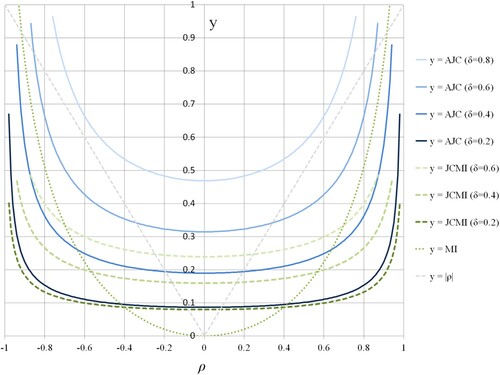
As the first of the numerical simulations, we investigate the feature of the Jaccard cell for the change of correlation coefficient ρ. Figure 3 shows the graphs of AJC (33(33) $\left(\mathrm{A}\mathrm{J}\mathrm{C}\right):\psi ({\mu }_x,{\mu }_y;\delta ,\delta )\approx \frac{\delta }{\sqrt{2\pi (1-{\rho }^2)}-\delta }.$(33) ) in $\delta =0.2,0.4,0.6,0.8$, JCMI (35(35) $\begin{array}{rl}& \left(\mathrm{J}\mathrm{C}\mathrm{M}\mathrm{I}\right):\psi ({\mu }_x,{\mu }_y;\delta ,\delta )\approx \frac{\delta }{\sqrt{2\pi (1-{\rho }^2)}}\\ & =\frac{\delta }{\sqrt{2\pi }}{\mathrm{e}}^{I(X,Y)}.\end{array}$(35) ) in $\delta =0.2,0.4,0.6$, MI (34(34) $I(X,Y)=-\frac{1}{2}\ln (1-{\rho }^2)=\ln \frac{1}{\sqrt{1-{\rho }^2}}.$(34) ), and the absolute value of the correlation coefficient $|\rho |$. By Figure 3, we can see that (33(33) $\left(\mathrm{A}\mathrm{J}\mathrm{C}\right):\psi ({\mu }_x,{\mu }_y;\delta ,\delta )\approx \frac{\delta }{\sqrt{2\pi (1-{\rho }^2)}-\delta }.$(33) ) is well-approximated by (35(35) $\begin{array}{rl}& \left(\mathrm{J}\mathrm{C}\mathrm{M}\mathrm{I}\right):\psi ({\mu }_x,{\mu }_y;\delta ,\delta )\approx \frac{\delta }{\sqrt{2\pi (1-{\rho }^2)}}\\ & =\frac{\delta }{\sqrt{2\pi }}{\mathrm{e}}^{I(X,Y)}.\end{array}$(35) ) based on MI in the small δ (i.e. $\delta =0.2$), but it is not so in $\delta =0.4$ and 0.6. Moreover, the condition (38(38) $0<\delta \le \sqrt{\frac{\pi }{2}(1-{\rho }^2)}\le \sqrt{\frac{\pi }{2}}.$(38) ) on δ constrains (33(33) $\left(\mathrm{A}\mathrm{J}\mathrm{C}\right):\psi ({\mu }_x,{\mu }_y;\delta ,\delta )\approx \frac{\delta }{\sqrt{2\pi (1-{\rho }^2)}-\delta }.$(33) ) and (35(35) $\begin{array}{rl}& \left(\mathrm{J}\mathrm{C}\mathrm{M}\mathrm{I}\right):\psi ({\mu }_x,{\mu }_y;\delta ,\delta )\approx \frac{\delta }{\sqrt{2\pi (1-{\rho }^2)}}\\ & =\frac{\delta }{\sqrt{2\pi }}{\mathrm{e}}^{I(X,Y)}.\end{array}$(35) ). Solving (38(38) $0<\delta \le \sqrt{\frac{\pi }{2}(1-{\rho }^2)}\le \sqrt{\frac{\pi }{2}}.$(38) ) for ρ, we obtain the bound of ρ for (33(33) $\left(\mathrm{A}\mathrm{J}\mathrm{C}\right):\psi ({\mu }_x,{\mu }_y;\delta ,\delta )\approx \frac{\delta }{\sqrt{2\pi (1-{\rho }^2)}-\delta }.$(33) ) and (35(35) $\begin{array}{rl}& \left(\mathrm{J}\mathrm{C}\mathrm{M}\mathrm{I}\right):\psi ({\mu }_x,{\mu }_y;\delta ,\delta )\approx \frac{\delta }{\sqrt{2\pi (1-{\rho }^2)}}\\ & =\frac{\delta }{\sqrt{2\pi }}{\mathrm{e}}^{I(X,Y)}.\end{array}$(35) ) as the following: (51) $|\rho |\le {\rho }_{\delta }:=\sqrt{1-\frac{2}{\pi }{\delta }^2}.$(51) Thus, the bounds in Figure 3 are ${\rho }_{0.2}\approx 0.987$, ${\rho }_{0.4}\approx 0.948$, ${\rho }_{0.6}\approx 0.878$, and ${\rho }_{0.8}\approx 0.770$. The values of the approximated Jaccard cells are flat in the range of the low and middle of $|\rho |$. It shows an abrupt increase in that of the high. Therefore, the Jaccard cell could strongly react to correlation locally formed in an appropriate small region.

Figure 3. The graphs of the Jaccard cells (JC) based on Equation (33(33) $\left(\mathrm{A}\mathrm{J}\mathrm{C}\right):\psi ({\mu }_x,{\mu }_y;\delta ,\delta )\approx \frac{\delta }{\sqrt{2\pi (1-{\rho }^2)}-\delta }.$(33) ) in $\delta =0.2,0.4,0.6,0.8$, the approximation by (35(35) $\begin{array}{rl}& \left(\mathrm{J}\mathrm{C}\mathrm{M}\mathrm{I}\right):\psi ({\mu }_x,{\mu }_y;\delta ,\delta )\approx \frac{\delta }{\sqrt{2\pi (1-{\rho }^2)}}\\ & =\frac{\delta }{\sqrt{2\pi }}{\mathrm{e}}^{I(X,Y)}.\end{array}$(35) ) in $\delta =0.2,0.4,0.6$, the MI (34(34) $I(X,Y)=-\frac{1}{2}\ln (1-{\rho }^2)=\ln \frac{1}{\sqrt{1-{\rho }^2}}.$(34) ), and the absolute value of the correlation coefficient $|\rho |$.

6.2. Jaccard matrix and the cell-size parameter uniquely determined by the standard deviation maximization

As the second of the numerical simulations, we investigate the mean $\overline{\psi }$, the variance $V_{\psi }$, and the standard deviation $\sqrt{V_{\psi }}$ of $n\times n$ Jaccard matrix, defined by (18(18) $\overline{\psi }:=\frac{1}{N_c}\sum _{i=0}^{n-1}\sum _{j=0}^{m-1}{\psi }_{ij}=\frac{{}^t{\mathbf{1}}_n\mathrm{\Psi }{\mathbf{1}}_m}{{}^t{\mathbf{1}}_{n}C{\mathbf{1}}_m}.$(18) ) and (19(19) $\begin{array}{rl}{V}_{\psi }& :=\frac{1}{N_c}\sum _{i=0}^{n-1}\sum _{j=0}^{m-1}{\psi }_{ij}^2-(\overline{\psi }{)}^2\\ & =\frac{{}^t{\mathbf{1}}_n(\mathrm{\Psi }\circ \mathrm{\Psi }){\mathbf{1}}_m}{{}^t{\mathbf{1}}_{n}C{\mathbf{1}}_m}-{\left(\frac{{}^t{\mathbf{1}}_n\mathrm{\Psi }{\mathbf{1}}_m}{{}^t{\mathbf{1}}_{n}C{\mathbf{1}}_m}\right)}^2,\end{array}$(19) ). We express the numerical values of them as $\mathrm{A}\mathrm{v}\mathrm{e}\left(\mathrm{\Psi }\right)$, $\mathrm{V}\left(\mathrm{\Psi }\right)$, and $\mathrm{S}\mathrm{D}\left(\mathrm{\Psi }\right)$. The input data set $\mathcal{D}=\left\{\right(x_i,y_i)|i=1,\dots ,N_c\}$ is generated by (52) $x=u\mathrm{a}\mathrm{n}\mathrm{d}y=f\left(x\right)+r,$(52) where u is a uniform random variable on an appropriately defined interval of real numbers and r is a noise defined as a normal random variable following $\mathrm{N}\mathrm{o}\mathrm{r}\mathrm{m}(0,{\sigma }_r^2)$. Table 3 expresses the instances of Equation (52(52) $x=u\mathrm{a}\mathrm{n}\mathrm{d}y=f\left(x\right)+r,$(52) ) to generate data $\mathcal{D}$. For each function f, we test the 30 data sets for the noise scales ${\sigma }_r={10}^{-a}$ ($a=0.1,0.2,\dots ,2.9,3.0$). The data size of $\mathcal{D}$ is $N_c=2\times {10}^4$.

Table 3. The instances of the function to generate test data.

Cos7x	$f\left(x\right)=\cos 7x$, $x\in [0,\pi ]$
Cos14x	$f\left(x\right)=\cos 14x$, $x\in [0,\pi ]$
Sin28x	$f\left(x\right)=\sin 28x$, $x\in [0,1]$
SinVaryingFreq	$f\left(x\right)=\sin \left\{7\pi x\right(x+1\left)\right\}$, $x\in [0,1]$
Parabola	$f\left(x\right)=x^2$, $x\in [-0.5,0.5]$
Cubic	$f\left(x\right)=x^3+x^2-4x$, $x\in [-1.3,1.1]$

Figure 4 shows the typical behaviour of $\mathrm{A}\mathrm{v}\mathrm{e}\left(\mathrm{\Psi }\right)$, $\mathrm{V}\left(\mathrm{\Psi }\right)$, and $\mathrm{S}\mathrm{D}\left(\mathrm{\Psi }\right)$ for n which defines $n\times n$ Jaccard matrix. These lines are generated by Equation (52(52) $x=u\mathrm{a}\mathrm{n}\mathrm{d}y=f\left(x\right)+r,$(52) ) using the function Cos14x in Table 3 and ${\sigma }_r={10}^{-3}$. Figure 5 shows the numerical tests for the theoretical model (46(46) $\begin{array}{rl}& =V\left[\phi \right]\left(\overline{\phi }\right)=-{(\overline{\phi }-\frac{Z_V}{2Z_E})}^2+\frac{Z_V^2}{4Z_E^2}\end{array}$(46) ) expressing the estimation of the relationship between the mean and the variance of the Jaccard cells. The plotted dots of it are generated by the function Cos14x of ${\sigma }_r={10}^{-3},{10}^{-2},{10}^{-1},{10}^{-0.1}$. The grey dashed line shows the parabolic function $\mathrm{V}\left(\mathrm{\Psi }\right)=-{\alpha }_0\left(\mathrm{A}\mathrm{v}\mathrm{e}\right(\mathrm{\Psi })-{\alpha }_1{)}^2+{\alpha }_2$, where ${\alpha }_0=0.6$, ${\alpha }_1=0.61$, and ${\alpha }_2=0.096$, to approximate the dots of ${\sigma }_r={10}^{-3}$ phenomenologically. Although the values of Figures 4 and 5 are the results of the function Cos14x, all of the instances in Table 3 show the behaviour qualitatively equivalent.

Figure 4. The typical behaviour of $\mathrm{A}\mathrm{v}\mathrm{e}\left(\mathrm{\Psi }\right)$, $\mathrm{V}\left(\mathrm{\Psi }\right)$, and $\mathrm{S}\mathrm{D}\left(\mathrm{\Psi }\right)$ for n which defines $n\times n$ Jaccard matrix. These lines are generated by Equation (52(52) $x=u\mathrm{a}\mathrm{n}\mathrm{d}y=f\left(x\right)+r,$(52) ) using the function Cos14x in Table 3 and ${\sigma }_r={10}^{-3}$.

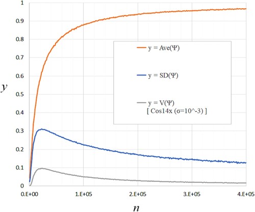
Figure 5. The numerical tests for the theoretical model (46(46) $\begin{array}{rl}& =V\left[\phi \right]\left(\overline{\phi }\right)=-{(\overline{\phi }-\frac{Z_V}{2Z_E})}^2+\frac{Z_V^2}{4Z_E^2}\end{array}$(46) ) expressing the estimation of the relationship between the mean and the variance of the Jaccard cells. The plotted dots are generated by the function Cos14x of ${\sigma }_r={10}^{-3},{10}^{-2},{10}^{-1},{10}^{-0.1}$. The grey dashed line shows the parabolic function $\mathrm{V}\left(\mathrm{\Psi }\right)=-{\alpha }_0\left(\mathrm{A}\mathrm{v}\mathrm{e}\right(\mathrm{\Psi })-{\alpha }_1{)}^2+{\alpha }_2$, where ${\alpha }_0=0.6$, ${\alpha }_1=0.61$, and ${\alpha }_2=0.096$, to approximate the dots of ${\sigma }_r={10}^{-3}$ phenomenologically.

The variances $\mathrm{V}\left(\mathrm{\Psi }\right)$ have the stationary points in the numerical simulations, like the parabolic function of the theoretical model (46(46) $\begin{array}{rl}& =V\left[\phi \right]\left(\overline{\phi }\right)=-{(\overline{\phi }-\frac{Z_V}{2Z_E})}^2+\frac{Z_V^2}{4Z_E^2}\end{array}$(46) ). Therefore, we can uniquely determine the value of the cell-size parameter and the Jaccard matrix not only in the theoretical model but also in the numerical calculation. Note that the results of simulations qualitatively correspond with that of the model but do not quantitively.

6.3. The standard deviation of the Jaccard cells as a nonlinear correlation

As the third of the numerical simulations, we investigate the relationship between the standard deviation of the Jaccard cells and that of the input data given by (52(52) $x=u\mathrm{a}\mathrm{n}\mathrm{d}y=f\left(x\right)+r,$(52) ), theoretically expressed by (50(50) $\log S{D}^{\ast }\propto -\log \sigma .$(50) ).

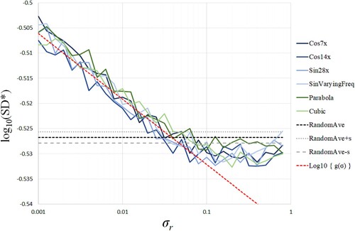
Figure 6 shows the values of ${\log }_{10}{\mathrm{S}\mathrm{D}}^{\ast }$ for the standard deviation ${\sigma }_r$ of the additional noise r of Equation (52(52) $x=u\mathrm{a}\mathrm{n}\mathrm{d}y=f\left(x\right)+r,$(52) ). Note the irregular representation of axes in Figure 6, i.e. the horizontal axis is a logarithmic one for the value of ${\sigma }_r$, and the vertical axis is a normal one for the value of ${\log }_{10}{\mathrm{S}\mathrm{D}}^{\ast }$ since the absolute value of the derivative of ${\mathrm{S}\mathrm{D}}^{\ast }$ is very small. ${\mathrm{S}\mathrm{D}}^{\ast }=\mathrm{S}\mathrm{D}\left({\mathrm{\Psi }}^{\ast }\right)$ means the stationary point of $\mathrm{S}\mathrm{D}\left(\mathrm{\Psi }\right)$ in Figure 5. All conditions of input data are the same as in the previous subsection. The horizontal dashed lines (RandomAve±s) in Figure 6 show the mean ± standard deviation values of ${\mathrm{S}\mathrm{D}}^{\ast }$ generated by 30 data sets of i.i.d. normal random numbers, $x,y\sim \mathrm{N}\mathrm{o}\mathrm{r}\mathrm{m}(0,1)$. In Figure 6, we can see the proportional trend (53) $\log {\mathrm{S}\mathrm{D}}^{\ast }\propto -\kappa \log {\sigma }_r$(53) in the range of ${10}^{-3}\le {\sigma }_r<{10}^{-1}$. The red dashed line expresses $y={\log }_{10}\left\{g\right({\sigma }_r\left)\right\}={\log }_{10}\left\{0.285{\sigma }_r^{-0.013}\right\}=-0.013{\log }_{10}{\sigma }_r+{\log }_{10}0.285$ as the approximation of $y={\log }_{10}{\mathrm{S}\mathrm{D}}^{\ast }$ in the range.

Figure 6. The values of ${\log }_{10}{\mathrm{S}\mathrm{D}}^{\ast }$ for the standard deviation ${\sigma }_r$ of the additional noise r of Equation (52(52) $x=u\mathrm{a}\mathrm{n}\mathrm{d}y=f\left(x\right)+r,$(52) ). The horizontal axis is a logarithmic one for the value of ${\sigma }_r$, and the vertical axis is a normal one for the value of ${\log }_{10}{\mathrm{S}\mathrm{D}}^{\ast }$.

The simple theoretical model (43(43) $\phi =\frac{{\delta }_0}{\text{β}-{\delta }_0}(0<{\delta }_0\le \text{β}/2).$(43) ) of the Jaccard cell predicts the relation (50(50) $\log S{D}^{\ast }\propto -\log \sigma .$(50) ) that corresponds to $\kappa =1$ in (53(53) $\log {\mathrm{S}\mathrm{D}}^{\ast }\propto -\kappa \log {\sigma }_r$(53) ), but the numerical results show $\kappa =0.013$. The trend of (53(53) $\log {\mathrm{S}\mathrm{D}}^{\ast }\propto -\kappa \log {\sigma }_r$(53) ) suggests that ${\mathrm{S}\mathrm{D}}^{\ast }$ might be used as an index of nonlinear correlation by the qualitative correspondence between the theoretical prediction and the numerical results, although it has a quantitative difference between them.

7. Discussion

In this section, we discuss the implications of the theoretical and numerical results in the previous analyses and summarize the view of our study as nonlinear filter statistics.

First, one of the informatically significant meanings of the Jaccard cell is the behaviour as the exponential function of MI, which is shown by Equations (35(35) $\begin{array}{rl}& \left(\mathrm{J}\mathrm{C}\mathrm{M}\mathrm{I}\right):\psi ({\mu }_x,{\mu }_y;\delta ,\delta )\approx \frac{\delta }{\sqrt{2\pi (1-{\rho }^2)}}\\ & =\frac{\delta }{\sqrt{2\pi }}{\mathrm{e}}^{I(X,Y)}.\end{array}$(35) ) and (41(41) $\begin{array}{rl}\psi ({\mu }_x,{\mu }_y;{\delta }_0,{\delta }_0)& \approx \frac{{\delta }_0}{({\sigma }_x+{\sigma }_y)\sqrt{\frac{\pi }{2}(1-{\rho }^2)}}\\ & =\frac{{\delta }_0}{{\sigma }_x+{\sigma }_y}\sqrt{\frac{2}{\pi }}{\mathrm{e}}^{I(X,Y)}.\end{array}$(41) ) theoretically and by Figure 3 numerically. The local correlation coefficient of the data relates the Jaccard cell to the MI. Interestingly, as a result, the indicators our method aggregates, the Jaccard cells, are related to MI, like MIC. By the effect of the exponential function, the Jaccard cell could more strongly sharpen the x−y dependence of the two-dimensional data than just the MI.

Second, the standard deviation of the data affects the value of the Jaccard cell. The approximated Jaccard cell (41(41) $\begin{array}{rl}\psi ({\mu }_x,{\mu }_y;{\delta }_0,{\delta }_0)& \approx \frac{{\delta }_0}{({\sigma }_x+{\sigma }_y)\sqrt{\frac{\pi }{2}(1-{\rho }^2)}}\\ & =\frac{{\delta }_0}{{\sigma }_x+{\sigma }_y}\sqrt{\frac{2}{\pi }}{\mathrm{e}}^{I(X,Y)}.\end{array}$(41) ) suggests elongating the data deviation to the direction of each axis decreases the value of the Jaccard cell. That means the localized data increase the value of the Jaccard cell more than the expanded data.

Third, we uniquely determine the Jaccard matrix depending on the cell-size parameters by selecting them as the stationary point of the variances $\mathrm{V}\left(\mathrm{\Psi }\right)$, although we potentially could give the values of the cell-size parameters arbitrarily. The variances $\mathrm{V}\left(\mathrm{\Psi }\right)$ have the stationary points in the numerical simulations, like the parabolic function of the theoretical model (46(46) $\begin{array}{rl}& =V\left[\phi \right]\left(\overline{\phi }\right)=-{(\overline{\phi }-\frac{Z_V}{2Z_E})}^2+\frac{Z_V^2}{4Z_E^2}\end{array}$(46) ). Note that the results of simulations qualitatively correspond with that of the model but do not quantitively. Thus, we will need to improve the model to analyse the feature of the Jaccard cell in future research.

Fourth, ${\mathrm{S}\mathrm{D}}^{\ast }$ at the stationary point determined by the above method is a decreasing function of the noise scale σ of the data under the constraint conditions. The proportionality (50(50) $\log S{D}^{\ast }\propto -\log \sigma .$(50) ) suggests it theoretically, and Figure 6 and the proportionality (53(53) $\log {\mathrm{S}\mathrm{D}}^{\ast }\propto -\kappa \log {\sigma }_r$(53) ) numerically. It means that we might be able to use ${\mathrm{S}\mathrm{D}}^{\ast }$ as an index of nonlinear correlation. MIC needs to vary the heterogeneous grid pattern on the computational procedure for each data. By contrast, the Jaccard matrix has a homogeneous rectangular grid pattern. The variance $\mathrm{V}\left(\mathrm{\Psi }\right)$ of the Jaccard matrix shows unimodality and has a stationary point as the above. Thus, it has good features for finding a solution potentially. As with the stationary point analysis of the above, the difference between theoretical and numerical values is a matter for further study.

The structure of our method is abstractly similar to that of a convolutional neural network (CNN) composed of a convolution layer and a pooling layer. CNN extracts features of input data by a convolution layer called a filter and synthesizes them by a pooling layer. The first layer of our method, making the Jaccard matrix, affects the information derived from input data as a “nonlinear filter” extracting their features, but it is not a convolution operation. The second layer of that calculates an index of nonlinear correlation. We guess that $S{D}^{\ast }$ could and should replace an alternative statistic to express nonlinear correlation better in future studies. The Jaccard matrix and the procedure of our method will have been effective yet in the case of the replaced index, since$\mathrm{V}\left(\mathrm{\Psi }\right)$ has the determining ability of the cell-size parameters by the unimodality. It is significant to characterize features of numerical data as low-dimensional measures when humans understand and judge the structure and order of the data. In this sense, each AI and statistics have roles for themselves, although they are closely related to modern statistical machine learning. We think nonlinear filters like the Jaccard matrix might work as efficient components of explainable AI and statistics.

8. Conclusion

In this article, we proposed the Jaccard matrix and the Jaccard cell as the element of that, defined them as the extended concepts of the Jaccard index, and theoretically and numerically analysed them. The data on the Euclidean plane can derive the Jaccard matrix as a sparse matrix.

The Jaccard index is well known as a classical index of similarity between two sets and is derived from the $2\times 2$ table describing two binary classes. The Jaccard matrix has $n\times n$ (generally $n\times m$) elements called the Jaccard cells. It is an extended concept of the classical Jaccard index and has the arbitrariness of the cell size to derive it from observed data on ${\mathbb{R}}^2$. We showed the Jaccard cell inherits the feature of similarity as the exponential function of MI. We theoretically and numerically confirmed that the local correlation coefficient of the data on the Euclidean plane relates the Jaccard cell to the MI.

Although one could potentially select an arbitrary cell size of the grid to make the Jaccard matrix, the knowledge we can obtain from the matrix decreases if the cell size is too big or too small to distinguish the data clusters appropriately. Therefore, the Jaccard matrix needs a computational procedure to determine the cell size within the appropriate scale. Maximizing the variance of the Jaccard cells supports determining the unique cell size, which value locates in the middle range of the parabolic function of the cell-size parameter.

Moreover, the Jaccard matrix could derive an index extracting nonlinear correlation of the data. The maximized standard deviation of the Jaccard cells as such an index is a decreasing function of the noise scale of the data under the constraint conditions. The ability to determine the homogeneous rectangular grid pattern of the Jaccard matrix might be a significant feature for finding nonlinear correlation.

The structure of our method is abstractly similar to that of a convolutional neural network. The first layer making the Jaccard matrix affects the information derived from input data as a nonlinear filter extracting their features. The second layer calculates an index of nonlinear correlation. We would summarize this study as that of a nonlinear filter working as an efficient component of explainable AI and statistics.

Acknowledgments

We are grateful to the editors and anonymous reviewers for giving valuable and dedicated comments to improve this research.

Disclosure statement

No potential conflict of interest was reported by the authors.

Additional information

Notes on contributors

Moto Kamiura

Moto Kamiura received B.Sc. in 2002 from Toho University, Japan; M.Sc. in 2004, and Ph.D. in Physics in 2007 from Kobe University, Japan. He was an assistant professor at Tokyo University of Science from 2008 to 2011; a Cooperative Researcher at the Research Institute of Electrical Communication, Tohoku University from 2010 to 2016; an assistant professor at Tokyo Denki University from 2011 to 2018; Co-Founder/Vice-President of Felixia Inc. in Japan from 2017 to the present. He is presently an associate professor at the Institute for Advanced Research and Education, Doshisha University, Japan.

Ryo Sekine

Ryo Sekine received B.Info. in 2016 and M.Info. in 2018 from Tokyo Denki University, Japan. He is presently an engineer at Japan Information Processing Service Co., Ltd., Japan.

Appendix

In the Appendix, we show the procedures to calculate the approximations of the Jaccard cell (26(26) $\begin{array}{rl}\psi (x,y;{\delta }_x,{\delta }_y)& =\frac{P_3}{P_1+P_2-P_3}\\ & =\frac{{\int }_{S_1\cap S_2}p(x,y)\mathrm{d}x\mathrm{d}y}{{\int }_{S_1\cup S_2}p(x,y)\mathrm{d}x\mathrm{d}y}.\end{array}$(26) ) under the conditions of small values for the cell-size parameters. By completing the square of the exponent of Equation (29(29) $\begin{array}{rl}p(x,y)& =\frac{1}{2\pi {\sigma }_x{\sigma }_y\sqrt{1-{\rho }^2}}\exp \{-\frac{1}{2(1-{\rho }^2)}\\ & \times [\frac{(x-{\mu }_x{)}^2}{{\sigma }_x^2}-2\rho \frac{(x-{\mu }_x)(y-{\mu }_y)}{{\sigma }_x{\sigma }_y}\\ & +\frac{(y-{\mu }_y{)}^2}{{\sigma }_y^2}]\}.\end{array}$(29) ), the two-dimensional normal distribution $p(x,y)$ with correlation coefficient ρ, we can transform it into the following: (A1) $\begin{array}{rl}p(x,y)& =\frac{1}{2\pi {\sigma }_x{\sigma }_y\sqrt{1-{\rho }^2}}\exp \{-\frac{(x-{\mu }_x{)}^2}{2{\sigma }_x^2}\}\\ & \times \exp \{-A_0{(y-h(x\left)\right)}^2\},\end{array}$(A1) where $A_0=\frac{1}{2{\sigma }_y^2(1-{\rho }^2)}$ and $h\left(x\right)=\rho \frac{{\sigma }_y}{{\sigma }_x}(x-{\mu }_x)+{\mu }_y$. Let us set the parts of Equation (A1(A1) $\begin{array}{rl}p(x,y)& =\frac{1}{2\pi {\sigma }_x{\sigma }_y\sqrt{1-{\rho }^2}}\exp \{-\frac{(x-{\mu }_x{)}^2}{2{\sigma }_x^2}\}\\ & \times \exp \{-A_0{(y-h(x\left)\right)}^2\},\end{array}$(A1) ) as (A2) $\begin{array}{rl}{A}_1& :=\frac{1}{2\pi {\sigma }_x{\sigma }_y\sqrt{1-{\rho }^2}}\mathrm{a}\mathrm{n}\mathrm{d}\\ A_2\left(x\right)& :=A_1\exp \{-\frac{(x-{\mu }_x{)}^2}{2{\sigma }_x^2}\},\end{array}$(A2) then the integral of (A1(A1) $\begin{array}{rl}p(x,y)& =\frac{1}{2\pi {\sigma }_x{\sigma }_y\sqrt{1-{\rho }^2}}\exp \{-\frac{(x-{\mu }_x{)}^2}{2{\sigma }_x^2}\}\\ & \times \exp \{-A_0{(y-h(x\left)\right)}^2\},\end{array}$(A1) ) gives the marginal probability density $p\left(x\right)$ as the following: (A3) $\begin{array}{rl}{\int }_{-\mathrm{\infty }}^{\mathrm{\infty }}p(x,y)\mathrm{d}y& =A_2\left(x\right){\int }_{-\mathrm{\infty }}^{\mathrm{\infty }}\exp \{-A_0{(y-h(x\left)\right)}^2\}\\ & =A_2\left(x\right)\sqrt{\frac{\pi }{A_0}}\\ & =\frac{1}{\sqrt{2\pi }{\sigma }_x}\exp \{-\frac{(x-{\mu }_x{)}^2}{2{\sigma }_x^2}\}=p\left(x\right).\end{array}$(A3) Assuming the cell-size parameter ${\delta }_x$ is sufficiently small (i.e. $0<{\delta }_x\ll 1$), we can obtain the following approximation of $p\left(x\right)$ around ${\mu }_x$: (A4) $p({\mu }_x\pm {\delta }_x)=\frac{1}{\sqrt{2\pi }{\sigma }_x}\exp \{-\frac{(\pm {\delta }_x{)}^2}{2{\sigma }_x^2}\}\approx \frac{1}{\sqrt{2\pi }{\sigma }_x},$(A4) therefore we obtain (A5) $P_1\left({\mu }_x\right)={\int }_{{\mu }_x-{\delta }_x}^{{\mu }_x+{\delta }_x}p\left(x\right)\mathrm{d}x\approx 2{\delta }_x\cdot p({\mu }_x\pm {\delta }_x)=\frac{{\delta }_x}{{\sigma }_x}\sqrt{\frac{2}{\pi }}.$(A5) By the same calculation based on the symmetry of x and y, assuming ${\delta }_y$ is sufficiently small (i.e. $0<{\delta }_y\ll 1$), we can obtain the following approximation of $p\left(y\right)$ around ${\mu }_y$: (A6) $P_2\left({\mu }_y\right)={\int }_{{\mu }_y-{\delta }_y}^{{\mu }_y+{\delta }_y}p\left(y\right)\mathrm{d}y\approx 2{\delta }_y\cdot p({\mu }_y\pm {\delta }_y)=\frac{{\delta }_y}{{\sigma }_y}\sqrt{\frac{2}{\pi }}.$(A6) In addition, assuming ${\delta }_x$ and ${\delta }_y$ are sufficiently small, we obtain the following approximation of $p(x,y)$ around $({\mu }_x,{\mu }_y)$: (A7) $\begin{array}{rl}& p({\mu }_x\pm {\delta }_x,{\mu }_y\pm {\delta }_y)\\ & =A_1\exp \{-\frac{1}{2(1-{\rho }^2)}[\frac{{\delta }_x^2}{{\sigma }_x^2}-2\rho \frac{(\pm {\delta }_x)(\pm {\delta }_y)}{{\sigma }_x{\sigma }_y}+\frac{{\delta }_y^2}{{\sigma }_y^2}]\}\\ & =A_1\exp \{-\frac{1\pm {\rho }^2}{1-{\rho }^2}{\delta }^2\}\approx A_1=\frac{1}{2\pi {\sigma }_x{\sigma }_y\sqrt{1-{\rho }^2}},\end{array}$(A7) therefore we obtain (A8) $\begin{array}{rl}{P}_3({\mu }_x,{\mu }_y)& ={\int }_{{\mu }_x-{\delta }_x}^{{\mu }_x+{\delta }_x}{\int }_{{\mu }_y-{\delta }_y}^{{\mu }_y+{\delta }_y}p(x,y)\mathrm{d}x\mathrm{d}y\\ & \approx \left(2{\delta }_x\right)\cdot \left(2{\delta }_y\right)\cdot p({\mu }_x\pm {\delta }_x,{\mu }_y\pm {\delta }_y)\\ & =\frac{2{\delta }_x{\delta }_y}{\pi {\sigma }_x{\sigma }_y\sqrt{1-{\rho }^2}}.\end{array}$(A8) Consequently, by Equations (A5(A5) $P_1\left({\mu }_x\right)={\int }_{{\mu }_x-{\delta }_x}^{{\mu }_x+{\delta }_x}p\left(x\right)\mathrm{d}x\approx 2{\delta }_x\cdot p({\mu }_x\pm {\delta }_x)=\frac{{\delta }_x}{{\sigma }_x}\sqrt{\frac{2}{\pi }}.$(A5) ), (A6(A6) $P_2\left({\mu }_y\right)={\int }_{{\mu }_y-{\delta }_y}^{{\mu }_y+{\delta }_y}p\left(y\right)\mathrm{d}y\approx 2{\delta }_y\cdot p({\mu }_y\pm {\delta }_y)=\frac{{\delta }_y}{{\sigma }_y}\sqrt{\frac{2}{\pi }}.$(A6) ), and (A8(A8) $\begin{array}{rl}{P}_3({\mu }_x,{\mu }_y)& ={\int }_{{\mu }_x-{\delta }_x}^{{\mu }_x+{\delta }_x}{\int }_{{\mu }_y-{\delta }_y}^{{\mu }_y+{\delta }_y}p(x,y)\mathrm{d}x\mathrm{d}y\\ & \approx \left(2{\delta }_x\right)\cdot \left(2{\delta }_y\right)\cdot p({\mu }_x\pm {\delta }_x,{\mu }_y\pm {\delta }_y)\\ & =\frac{2{\delta }_x{\delta }_y}{\pi {\sigma }_x{\sigma }_y\sqrt{1-{\rho }^2}}.\end{array}$(A8) ), we obtain the following approximation of the Jaccard cell (30(30) $\begin{array}{rl}\psi ({\mu }_x,{\mu }_y;{\delta }_x,{\delta }_y)& =\frac{P_3({\mu }_x,{\mu }_y)}{P_1\left({\mu }_x\right)+P_2\left({\mu }_y\right)-P_3({\mu }_x,{\mu }_y)}\\ & \approx \frac{{\delta }_x{\delta }_y}{({\delta }_x{\sigma }_y+{\delta }_y{\sigma }_x)\sqrt{\frac{\pi }{2}(1-{\rho }^2)}-{\delta }_x{\delta }_y}.\end{array}$(30) ).

References

- Pearson K. Notes on the history of correlation. Biometrika. 1920;13(1):25–45.
- Speed T. A correlation for the 21st century. Science. 2011;334(6062):1502–1503.
- Reshef DN, Reshef YA, Finucane HK, et al. Detecting novel associations in large data sets. Science. 2011;334(6062):1518–1524.
- Chen Y, Zeng Y, Luo F, et al. A new algorithm to optimize maximal information coefficient. PLoS ONE. 2016;11(6):e0157567.
- Zhang ZX, Hao W, Chen G, et al. An extension of MIC for multivariate correlation analysis based on interaction information. In: CSAI'18: Proceedings of the 2018 Second International Conference on Computer Science and Artificial Intelligence. 2018. p. 399–403. Shenzhen, China.
- Jaccard P. The distribution of the flora in the alpine zone. New Phytol. 1912;11(2):37–50.
- Tanimoto TT. An elementary mathematical theory of classification and prediction. IBM Internal; 1958. (Technical report).
- Tversky A. Features of similarity. Psychol Rev. 1977;84(4):327–352.
- Takahashi T, Kohno Y, Oyo K. Causal induction heuristics as proportion of assumed-tobe rare instances (pARIs). In: Proceedings of the Seventh International Conference on Cognitive Science. 2010. p. 361–362. Beijing, China.
- Kamiura M, Takahashi T. Informatics of a stochastic model for causal induction. In: Proceeding of the 27th Annual Conference of the Japanese Society for Artificial Intelligence. 2013. 1L5OS24c3 p. 1–3. Toyama, Japan.
- Takahashi T. Correlation detection with and without the theories of conditionals, in logic and uncertainty in the human mind: a tribute to David E. Over. New York, NY: Routledge; 2020. p. 207–226.
- Higuchi K, Oyo K, Takahashi T. Causal intuition in the indefinite world: meta-analysis and simulations. Biosystems. 2023;225:104842.
- Sloman SA, Lagnado D. Causality in thought. Annu Rev Psychol. 2015;66:223–247.
- Hattori M, Oaksford M. Adaptive non-interventional heuristics for covariation detection in causal induction: model comparison and rational analysis. Cogn Sci. 2007;31:765–814.
- Kamiura M. pARIX: an index for causal induction as extended pARIs/JACCARD index. In: Proceedings of the SICE Annual Conference 2014. p. 872–876. Sapporo, Japan.
- Kamiura M. Jaccard matrix supporting calculations of nonlinear correlation. In: Proceedings of the 21st International Symposium on Artificial Life and Robotics (AROB). 2016. OS14-3. Beppu, Japan.
- Murphy KP. Machine learning: a probabilistic perspective. Cambridge, Mass: MIT Press; 2012. p. 35.
- Saad Y. Iterative methods for sparse linear systems. Philadelphia, Penn: SIAM; 2003.
- Buluç A, Fineman JT, Frigo M, et al. Parallel sparse matrix-vector and matrix-transpose-vector multiplication using compressed sparse blocks. In: Proceedings of the 21st Annual Symposium on Parallelism in Algorithms and Architectures (SPAA09). 2009. p. 233–244. Calgary, Canada.