Sampled visual feedback pose estimation and regulation based on camera frame rates

ABSTRACT

This paper presents visual feedback 3D pose estimation/regulation methodologies in the sampled data setting by camera frame rates. Vision-based estimation/control problems have been studied by a number of research groups. While most works focus on the limitation of measured outputs, they conduct convergence/performance analysis under the assumption that visual measurements extracted from a camera are continuously available. However, the camera frame rates including image processing time often cannot be neglected compared with other computation time. In view of this fact, this paper newly proposes visual feedback pose estimation/regulation techniques under the situation that visual measurements are sampled due to the frame rates. The problem settings are first provided. Then, the pose estimation/regulation methods with sampled visual measurements are proposed. The convergence/performance analysis is conducted by the fusion of a Lyapunov-based approach and an event-triggered control technique. The present analysis scheme provides us guidelines for the design of estimation/control gains guaranteeing desired convergence/performance. The effectiveness of the present technique is verified via simulation and an experiment with real hardware.

KEYWORDS:

• Vision-based control
• rigid body motion
• passivity
• event-triggered control
• sampled data setting

1. Introduction

Vision sensors have been widely leveraged for situation recognition since they provide rich 2D information projected from 3D relative states [1]. Thanks to this utility, vision sensors are also utilized in robotics and control engineering communities to develop vision-based autonomous control methods [2–12]. In vision-based control, one of the main issues is how to deal with 2D visual information to estimate/control a 3D pose (position and orientation) of a target object (relative to a camera) [5,10–12]. On the other hand, compared with other computation times, the sampling time for extracting desired information from the image, i.e. a camera frame rate, might not be small enough to be neglected, especially when complex image processing algorithms are employed. Nonetheless, most of research studies, including the references above, focus only on the limitation of measured outputs for estimation/control under the premise that visual information is continuously available.

In view of this fact, this paper investigates visual feedback 3D pose estimation/regulation problems in the sampled data setting. Here, the objectives are (i) to estimate the 3D target object pose relative to the camera, and (ii) to drive the relative pose to a desired one, by using only sampled 2D visual information extracted from a monocular camera with a certain frame rate. To achieve these goals, we introduce a visual feedback 3D pose estimation mechanism, called a visual motion observer, presented by [13,14] and also utilized for some extended estimation/control objectives [15–17]. In the visual motion observer, a passivity property of rigid body motion plays a central role and estimation/control performance is analysed through a Lyapunov-based approach. However, similarly to the references above, the observer assumes continuous measurements of visual information. This assumption leads to the convergence/performance analysis allowing any large positive estimation/control gains, but high gain estimation and its control application often do not work in real experiments with sampled measurements. Therefore, this paper extends the visual motion observer to that with sampled visual measurements.

Since the observer input is formed by the visual measurements, the input is also sampled in the case of sampled measurements. For conducting convergence/performance analysis even in the sampled data setting, this paper employs an event-triggered control technique [18–20]. The merit of event-triggered control is the possibility to reduce the number of re-computing inputs and transmissions (i.e. events) while guaranteeing desired performance. Specifically, inter-event time is investigated to guarantee a monotonic decrease of Lyapunov-like functions for convergence. This technique is suited to the visual motion observer because its convergence/performance analysis is also based on non-increasing properties of Lyapunov-like functions. As a result of the event-triggered approach, we can obtain gain limitations for desired convergence/performance based on given certain camera frame rates.

In summary, the main contribution of this work is to propose a novel vision-based pose observer and its control application in the sampled data setting by camera frame rates. We first provide problem settings: a 3D relative motion model between a camera and a target object; a visual measurement model; and definitions of the estimation and control objectives. Then, we newly propose a sampled visual motion observer and give convergence analysis for the stationary target object case and tracking analysis for the moving object case. A pose regulation method based on the proposed sampled visual motion observer is next proposed, and the regulation/tracking analysis is also conducted for the stationary/moving object. Here, we provide the relationship between the frame rates and estimation/control gains to achieve desired convergence/performance. Specifically, we show that estimation and control errors are ultimately bounded by a function of the camera frame rate, estimation/control gains and target object velocity. This analysis provides us with the guidelines for gain settings. The effectiveness of the proposed methods is demonstrated via simulation and an experiment with real hardware.

The conference versions of this paper are reported in [21,22]. While [21] considers only estimation problems, this work also tackles pose regulation problems. Compared with [22], we greatly improve the conservativeness of the gain condition by modifying the control law structure, and newly carrying out an experimental demonstration with real hardware.

2. Problem settings

This section formulates 3D visual feedback pose estimation/regulation problems consisting of two rigid bodies (a camera robot and a target object robot) and visual measurements by a monocular camera.

2.1. Relative rigid body motion

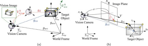
Throughout this paper, this work considers a visual feedback system shown in Figure 1. Let the world frame, camera frame, and object frame be ${\mathrm{\Sigma }}_w$, ${\mathrm{\Sigma }}_c$, and ${\mathrm{\Sigma }}_o$, respectively (see Figure 1(a)). Then, the pose of the origin of ${\mathrm{\Sigma }}_c$ relative to ${\mathrm{\Sigma }}_w$ is represented by $g_{wc}=(p_{wc},e^{{\hat{\xi }}_{wc}{\theta }_{wc}})\in SE\left(3\right)$, where $SE\left(3\right):={\mathbb{R}}^3\times SO\left(3\right)$, $SO\left(3\right):=\{R\in {\mathbb{R}}^{3\times 3}\mid R^{\mathrm{T}}R=I_3,detR=1\}$. ($I_n\in {\mathbb{R}}^{n\times n}$ is the n-dimensional identity matrix.) The orientation is represented by the exponential coordinate of the rotation matrix with the unit axis ${\xi }_{wc}\in {\mathbb{R}}^3$ $({\xi }_{wc}^{\mathrm{T}}{\xi }_{wc}=1)$ and the angle ${\theta }_{wc}\in (-\pi ,\pi ]$. The operator $\wedge :{\mathbb{R}}^3\to so\left(3\right)$, $so\left(3\right):=\{S\in {\mathbb{R}}^{3\times 3}\mid S^{\mathrm{T}}=-S\}$ provides $\hat{a}b=a\times b,a,b\in {\mathbb{R}}^3$ for the vector cross-product “×,” and $\vee :so\left(3\right)\to {\mathbb{R}}^3$ is its inverse operator. For the ease of representation, ${\xi }_{wc}{\theta }_{wc}$ is simply written by $\xi {\theta }_{wc}$ in this paper. Similarly, the pose of ${\mathrm{\Sigma }}_o$ relative to ${\mathrm{\Sigma }}_w$ is represented by $g_{wo}=(p_{wo},e^{\hat{\xi }{\theta }_{wo}})\in SE\left(3\right)$.

Figure 1. Visual feedback system. (a) Coordinate frames and (b) Perspective projection model.

Let us next introduce the body velocity of ${\mathrm{\Sigma }}_c$ relative to ${\mathrm{\Sigma }}_w$ as $V_{wc}^b=[v_{wc}^{\mathrm{T}}{\omega }_{wc}^{\mathrm{T}}{]}^{\mathrm{T}}\in {\mathbb{R}}^6$ and that of ${\mathrm{\Sigma }}_o$ as $V_{wo}^b=[v_{wo}^{\mathrm{T}}{\omega }_{wo}^{\mathrm{T}}{]}^{\mathrm{T}}\in {\mathbb{R}}^6$. Here, $v\in {\mathbb{R}}^3$ and $\omega \in {\mathbb{R}}^3$ are respectively the body translational velocity and angular one. The pose g and body velocity $V^b$ can be also written in the homogeneous representation form as follows: $\begin{array}{rl}g& =\left[\begin{array}{cc}{e}^{\hat{\xi }\theta }& p\\ O_{1\times 3}& 1\end{array}\right]\in {\mathbb{R}}^{4\times 4},\\ {\hat{V}}^b& =\left[\begin{array}{cc}\hat{\omega }& v\\ O_{1\times 3}& 0\end{array}\right]\in {\mathbb{R}}^{4\times 4}.\end{array}$($O_{m\times n}\in {\mathbb{R}}^{m\times n}$ represents the $m\times n$ zero matrix.) Notice here that another definition of “$\wedge$” is used for the 6D vector $V^b$. Then, $V_{wc}^b$ and $V_{wo}^b$ are respectively given by ${\hat{V}}_{wc}^b=g_{wc}^{-1}{\dot{g}}_{wc}$ and ${\hat{V}}_{wo}^b=g_{wo}^{-1}{\dot{g}}_{wo}$ [1].

Similarly, the pose of ${\mathrm{\Sigma }}_o$ relative to ${\mathrm{\Sigma }}_c$ and its body velocity are denoted by $g_{co}=(p_{co},e^{\hat{\xi }{\theta }_{co}})\in SE\left(3\right)$ and $V_{co}^b:=(g_{co}^{-1}{\dot{g}}_{co}{)}^{\vee }\in {\mathbb{R}}^6$, respectively. Then, $g_{co}=g_{wc}^{-1}{g}_{wo}$ holds, and thus the following relative rigid body motion is obtained from ${\hat{V}}_{co}^b=g_{co}^{-1}{\dot{g}}_{co}$: (1) ${\dot{g}}_{co}=-{\hat{V}}_{wc}^b{g}_{co}+g_{co}{\hat{V}}_{wo}^b.$(1)

2.2. Visual measurements

2D visual measurements extracted from a monocular camera are introduced as the measured outputs for 3D pose estimation/regulation laws. Although the extraction by perspective projection is only introduced in this paper, it can be easily extended to the panoramic camera case as in [15].

Consider the target object with $m(\ge 4)$ feature points. The positions of the feature points relative to the object frame ${\mathrm{\Sigma }}_o$ are represented by $p_{oi}\in {\mathbb{R}}^3,i\in \{1,\dots ,m\}$. Then, these positions relative to the camera frame ${\mathrm{\Sigma }}_c$ are given by $p_{ci}=g_{co}{p}_{oi}$ from the coordinate transformation.¹ We next denote the m feature points on the 2D image plane by $f=[f_1^{\mathrm{T}}\cdots f_m^{\mathrm{T}}{]}^{\mathrm{T}}\in {\mathbb{R}}^{2m}$. Then, the well-known perspective projection [1] yields the following relationship for each $f_i\in {\mathbb{R}}^2$ (see Figure 1(b)): (2) $f_i=\frac{\sigma }{z_{ci}}\left[\begin{array}{c}{x}_{ci}\\ y_{ci}\end{array}\right],p_{ci}=[x_{ci}{y}_{ci}{z}_{ci}{]}^{\mathrm{T}},i\in \{1,\dots ,m\}.$(2) Here, $\sigma >0$ is the focal length of the camera.

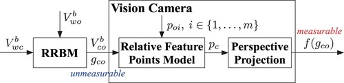
This paper considers the situation that the visual measurements f are only available for pose estimation/regulation laws, and supposes that the positions of the feature points in ${\mathrm{\Sigma }}_o$ (i.e. $p_{oi}$) are known a priori. Then, the visual measurements are given by the function only of the relative pose $g_{co}$, i.e. $f\left(g_{co}\right)$. Figure 2 illustrates the block diagram of the relative rigid body motion (1(1) ${\dot{g}}_{co}=-{\hat{V}}_{wc}^b{g}_{co}+g_{co}{\hat{V}}_{wo}^b.$(1) ) with the perspective projection (2(2) $f_i=\frac{\sigma }{z_{ci}}\left[\begin{array}{c}{x}_{ci}\\ y_{ci}\end{array}\right],p_{ci}=[x_{ci}{y}_{ci}{z}_{ci}{]}^{\mathrm{T}},i\in \{1,\dots ,m\}.$(2) ).

Figure 2. Block diagram of relative rigid body motion (RRBM) with camera model.

2.3. Research objectives

For the present visual feedback system, the objectives of this paper are

1. to propose a pose estimation mechanism of the relative pose $g_{co}$

2. to propose a pose regulation mechanism to drive $g_{co}$ to the fixed desired pose $g_d=(p_d,e^{\hat{\xi }{\theta }_d})\in SE\left(3\right)$ (see Figure 1(a))

under the situation that only the visual measurements $f\left(g_{co}\right)$ are available and the camera frame rates including the image processing time are non-negligible.

3. Sampled visual feedback pose estimation

We first propose a sampled visual feedback pose estimation mechanism taking account of camera frame rates for the objective (i).

3.1. Estimation error system

Since the 2D visual measurements (2(2) $f_i=\frac{\sigma }{z_{ci}}\left[\begin{array}{c}{x}_{ci}\\ y_{ci}\end{array}\right],p_{ci}=[x_{ci}{y}_{ci}{z}_{ci}{]}^{\mathrm{T}},i\in \{1,\dots ,m\}.$(2) ) are only available, we consider the estimation of the 3D relative pose $g_{co}$ by a nonlinear observer. The estimate of $g_{co}$ is represented by ${\overline{g}}_{co}=({\overline{p}}_{co},e^{\hat{\overline{\xi }}{\overline{\theta }}_{co}})\in SE\left(3\right)$. Similarly to the Luenberger-type observer [23], we build the copy model of the relative rigid body motion (1(1) ${\dot{g}}_{co}=-{\hat{V}}_{wc}^b{g}_{co}+g_{co}{\hat{V}}_{wo}^b.$(1) ) as follows: (3) ${\dot{\overline{g}}}_{co}=-{\hat{V}}_{wc}^b{\overline{g}}_{co}+{\overline{g}}_{co}{\hat{u}}_e.$(3) Here, $u_e=[u_{ep}^{\mathrm{T}}{u}_{eR}^{\mathrm{T}}{]}^{\mathrm{T}}\in {\mathbb{R}}^6$ is the observer input for the estimation of $g_{co}$. We note that the model (3(3) ${\dot{\overline{g}}}_{co}=-{\hat{V}}_{wc}^b{\overline{g}}_{co}+{\overline{g}}_{co}{\hat{u}}_e.$(3) ) does not include the target object velocity information $V_{wo}^b$, because it is unavailable.² Notice also that the estimated visual measurements $\overline{f}\in {\mathbb{R}}^{2m}$ can be computed by ${\overline{g}}_{co}$ and (2(2) $f_i=\frac{\sigma }{z_{ci}}\left[\begin{array}{c}{x}_{ci}\\ y_{ci}\end{array}\right],p_{ci}=[x_{ci}{y}_{ci}{z}_{ci}{]}^{\mathrm{T}},i\in \{1,\dots ,m\}.$(2) ).

Let us define the estimation error $g_{ee}=(p_{ee},e^{\hat{\xi }{\theta }_{ee}})\in SE\left(3\right)$ between $g_{co}$ and ${\overline{g}}_{co}$ and its vector form $e_e\in {\mathbb{R}}^6$ as follows: $g_{ee}:={\overline{g}}_{co}^{-1}{g}_{co},e_e:=\left[\begin{array}{c}{p}_{ee}\\ \mathrm{s}\mathrm{k}(e^{\hat{\xi }{\theta }_{ee}}{)}^{\vee }\end{array}\right].$Here, $\mathrm{s}\mathrm{k}\left(e^{\hat{\xi }\theta }\right):=\left(1/2\right)(e^{\hat{\xi }\theta }-e^{-\hat{\xi }\theta })\in so\left(3\right)$. The estimation error vector has the important property that for ${\theta }_{ee}\in (-\pi ,\pi )$, $e_e=0$ holds³ if and only if $g_{ee}=I_4$ which is equivalent to ${\overline{g}}_{co}=g_{co}$, i.e. the objective (i) is achieved. It should be also noted that $e_e$ can be approximately reconstructed by the measurement error $f_e:=f-\overline{f}\in {\mathbb{R}}^{2m}$ (refer to [13] for the details). Then, the time derivative of $g_{ee}$ along the trajectories of (1(1) ${\dot{g}}_{co}=-{\hat{V}}_{wc}^b{g}_{co}+g_{co}{\hat{V}}_{wo}^b.$(1) ) and (3(3) ${\dot{\overline{g}}}_{co}=-{\hat{V}}_{wc}^b{\overline{g}}_{co}+{\overline{g}}_{co}{\hat{u}}_e.$(3) ) yields the following estimation error system: (4) ${\dot{g}}_{ee}=-{\hat{u}}_e{g}_{ee}+g_{ee}{\hat{V}}_{wo}^b.$(4) This is also given in the vector form with the Adjoint transformation ${\mathrm{A}\mathrm{d}}_{\left(g\right)}\in {\mathbb{R}}^{6\times 6}$ as (5) $\begin{array}{rl}& V_{ee}^b:=(g_{ee}^{-1}{\dot{g}}_{ee}{)}^{\vee }=-{\mathrm{A}\mathrm{d}}_{\left(g_{ee}^{-1}\right)}{u}_e+V_{wo}^b,\\ & {\mathrm{A}\mathrm{d}}_{\left(g\right)}:=\left[\begin{array}{cc}{e}^{\hat{\xi }\theta }& \hat{p}{e}^{\hat{\xi }\theta }\\ O_{3\times 3}& e^{\hat{\xi }\theta }\end{array}\right].\end{array}$(5) Then, it is shown in [13] that if $V_{wo}^b=0$, the estimation error system (4(4) ${\dot{g}}_{ee}=-{\hat{u}}_e{g}_{ee}+g_{ee}{\hat{V}}_{wo}^b.$(4) ) has a passivity-like property from the input $u_e$ to the output $-e_e$ with the storage function $U_e\ge 0$, i.e. ${\dot{U}}_e=u_e^{\mathrm{T}}(-e_e)$ holds. Here, $\begin{array}{rl}& U_e:=\frac{1}{2}\Vert p_{ee}{\Vert }^2+\varphi \left(e^{\hat{\xi }{\theta }_{ee}}\right),\\ & \varphi \left(e^{\hat{\xi }{\theta }_{ee}}\right):=\frac{1}{4}\Vert I_3-e^{\hat{\xi }{\theta }_{ee}}{\Vert }_F^2=\frac{1}{2}\mathrm{t}\mathrm{r}(I_3-e^{\hat{\xi }{\theta }_{ee}})\ge 0,\end{array}$and notice that $U_e=0$ is equivalent to $e_e=0$, that is, the pose estimation (the objective (i)) is achieved. ($\Vert \cdot {\Vert }_F$ represents the Frobenius norm.) Based on this property, Fujita et al. [13] propose the following negative feedback law to achieve the pose estimation: $u_e=-k_e(-e_e)=k_e{e}_e,k_e>0,$where the achievement of the estimation is proved by the direct use of the storage function $U_e$ as a potential function for the Lyapunov-based energy approach. However, this observer input assumes that the visual measurements f are continuously available although general cameras have 60, 30, 15, or fewer fps when the image processing time to extract the feature points is included. Therefore, this paper tackles a new visual feedback pose estimation problem explicitly taking account of the camera frame rates.

3.2. Pose estimation mechanism

Let us first consider the case that the camera has a fixed frame rate $\tau >0$ [fps], and, for ease of representation, this includes the image processing time to extract the feature points. The variable frame rate case is handled at the end of the main results. We assume that the computation time to calculate the estimation input is small enough to be neglected compared with $1/\tau$. Then, based on the frame rate τ, we introduce the sampling time sequence $\{t_0,t_1,t_2,\dots \}$ such that $t_{i+1}-t_i=1/\tau$ holds for all $i\in {\mathbb{N}}_0$. (${\mathbb{N}}_0$ represents the union of natural numbers and $\left\{0\right\}$.) Then, the visual measurements (2(2) $f_i=\frac{\sigma }{z_{ci}}\left[\begin{array}{c}{x}_{ci}\\ y_{ci}\end{array}\right],p_{ci}=[x_{ci}{y}_{ci}{z}_{ci}{]}^{\mathrm{T}},i\in \{1,\dots ,m\}.$(2) ) are extracted at each time instant $t_i$.

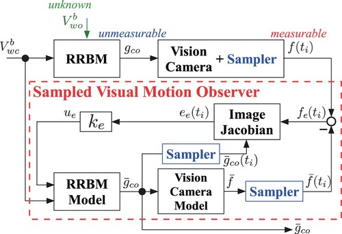
We now propose the following sampled observer input for the relative rigid body motion model (3(3) ${\dot{\overline{g}}}_{co}=-{\hat{V}}_{wc}^b{\overline{g}}_{co}+{\overline{g}}_{co}{\hat{u}}_e.$(3) ): (6) $u_e\left(t\right)=k_e{e}_e\left(t_i\right),t\in [t_i,t_{i+1}),k_e>0.$(6) Notice here that the present input remains to be constant until it is re-computed. Figure 3 illustrates the block diagram of the present estimation mechanism called the sampled visual motion observer. In the present observer since the image Jacobian consists of the estimates $\overline{f}$ and ${\overline{g}}_{co}$ as well as the visual measurements f [13], we employ the same samplers for these estimates as for the camera.

Figure 3. Block diagram of sampled visual motion observer.

4. Analysis of pose estimation

This section provides the convergence analysis for the stationary target object (i.e. $V_{wo}^b\equiv 0$ holds) and the tracking performance analysis for the moving target.

4.1. Convergence analysis

Let us define the sampling error $ϵ\left(t\right)\in {\mathbb{R}}^6$ between the actual estimation error $e_e\left(t\right)$ and the sampled one $e_e\left(t_i\right)$ as $ϵ\left(t\right):=e_e\left(t\right)-e_e\left(t_i\right),t\in [t_i,t_{i+1}){}^{\mathrm{\forall }}i\in {\mathbb{N}}_0.$Then, we obtain the following theorem:

Theorem 4.1

Suppose that the target object is static (i.e. $V_{wo}^b\equiv 0$). Then, if the camera frame rate satisfies the condition (7) $\tau \ge \frac{2k_e(1+\delta )}{\delta },\delta \in (0,1),$(7) there exist finite time $T_a\ge t_0$ and positive scalars ${\alpha }_1,{\text{β}}_1>0$ such that (8) $\Vert e_e\left(t\right)\Vert \le {\alpha }_1{e}^{-{\text{β}}_1(t-T_a)\mathrm{\forall }}t\ge T_a$(8) for the closed-loop system (4(4) ${\dot{g}}_{ee}=-{\hat{u}}_e{g}_{ee}+g_{ee}{\hat{V}}_{wo}^b.$(4) ) and (6(6) $u_e\left(t\right)=k_e{e}_e\left(t_i\right),t\in [t_i,t_{i+1}),k_e>0.$(6) ). In other words, the equilibrium point $e_e=0$ is exponentially stable after time $T_a$.

Proof.

When $V_{wo}^b=0$ holds, the time derivative of the potential function $U_e$ along the trajectories of (4(4) ${\dot{g}}_{ee}=-{\hat{u}}_e{g}_{ee}+g_{ee}{\hat{V}}_{wo}^b.$(4) ) and (6(6) $u_e\left(t\right)=k_e{e}_e\left(t_i\right),t\in [t_i,t_{i+1}),k_e>0.$(6) ) for $t\in [t_i,t_{i+1})$ yields $\begin{array}{rl}& {\dot{U}}_e=-e_e^{\mathrm{T}}{u}_e=-k_e{e}_e^{\mathrm{T}}{e}_e\left(t_i\right)=-k_e{e}_e^{\mathrm{T}}(e_e-ϵ)\\ & \le -k_e\Vert e_e{\Vert }^2+k_e\Vert e_e\Vert \Vert ϵ\Vert .\end{array}$Therefore, if the inequality (9) $\Vert ϵ\Vert \le \delta \Vert e_e\Vert ,\delta \in (0,1)$(9) is satisfied, we obtain (10) ${\dot{U}}_e\le -k_e(1-\delta )\Vert e_e{\Vert }^2\le 0$(10) for $t\in [t_i,t_{i+1})$.

We next derive the frame rate condition to guarantee the inequality (9(9) $\Vert ϵ\Vert \le \delta \Vert e_e\Vert ,\delta \in (0,1)$(9) ). Notice first that it is enough to consider each time interval $[t_i,t_{i+1})$ since ϵ becomes 0 at the next time step $t_{i+1}$. Motivated by the analysis of event-triggered control [18–20], we investigate the dynamics of $\Vert ϵ\Vert /\Vert e_e\Vert$ for $t\in [t_i,t_{i+1})$ as follows: (11) $\begin{array}{rl}\frac{\mathrm{d}}{\mathrm{d}t}\frac{\Vert ϵ\Vert }{\Vert e_e\Vert }& =\frac{{ϵ}^{\mathrm{T}}\dot{ϵ}\Vert e_e\Vert }{\Vert ϵ\Vert \Vert e_e{\Vert }^2}+\frac{\Vert ϵ\Vert e_e^{\mathrm{T}}{\dot{e}}_e}{\Vert e_e{\Vert }^3}\le \frac{\Vert {\dot{e}}_e\Vert }{\Vert e_e\Vert }\\ & +\frac{\Vert ϵ\Vert \Vert {\dot{e}}_e\Vert }{\Vert e_e{\Vert }^2}=(1+\frac{\Vert ϵ\Vert }{\Vert e_e\Vert })\frac{\Vert {\dot{e}}_e\Vert }{\Vert e_e\Vert }.\end{array}$(11) Here, we use the fact that $\dot{ϵ}={\dot{e}}_e$ for $t\in [t_i,t_{i+1})$. Let us now consider ${\dot{e}}_e$. Then, we first get the following position term from the estimation error system (4(4) ${\dot{g}}_{ee}=-{\hat{u}}_e{g}_{ee}+g_{ee}{\hat{V}}_{wo}^b.$(4) ) with $V_{wo}^b=0$: ${\dot{p}}_{ee}=-u_{ep}-{\hat{u}}_{eR}{p}_{ee}.$Before obtaining the orientation term, we note that the following equality holds for any vector $a\in {\mathbb{R}}^3$ and any matrix $A\in {\mathbb{R}}^{3\times 3}$: $\hat{a}A+A^{\mathrm{T}}\hat{a}=\left(\right(\mathrm{t}\mathrm{r}\left(A\right)I_3-A)a{)}^{\wedge }.$From this property and the estimation error system (4(4) ${\dot{g}}_{ee}=-{\hat{u}}_e{g}_{ee}+g_{ee}{\hat{V}}_{wo}^b.$(4) ) with $V_{wo}^b=0$, we get $\begin{array}{rl}& \frac{\mathrm{d}}{\mathrm{d}t}\left(\mathrm{s}\mathrm{k}\right(e^{\hat{\xi }{\theta }_{ee}}{)}^{\vee })\\ & =\frac{1}{2}({\dot{e}}^{\hat{\xi }{\theta }_{ee}}-{\dot{e}}^{-\hat{\xi }{\theta }_{ee}}{)}^{\vee }\\ & =\frac{1}{2}(e^{\hat{\xi }{\theta }_{ee}}{\hat{\omega }}_{ee}+{\hat{\omega }}_{ee}{e}^{-\hat{\xi }{\theta }_{ee}}{)}^{\vee }\\ & =\frac{1}{2}\left(\mathrm{t}\mathrm{r}\right(e^{-\hat{\xi }{\theta }_{ee}})I_3-e^{-\hat{\xi }{\theta }_{ee}}){\omega }_{ee}\\ & =-\frac{1}{2}{e}^{-\hat{\xi }{\theta }_{ee}}\left(\right(1+2\cos {\theta }_{ee})I_3-e^{-\hat{\xi }{\theta }_{ee}})u_{eR}.\end{array}$Here, we use the notation $V_{ee}^b=[v_{ee}^{\mathrm{T}}{\omega }_{ee}^{\mathrm{T}}{]}^{\mathrm{T}}$, and the representation $ϵ=[{ϵ}_p^{\mathrm{T}}{ϵ}_R^{\mathrm{T}}{]}^{\mathrm{T}}$ is also utilized hereafter. Therefore, using the properties $\Vert e^{\hat{\xi }\theta }\Vert =1$ and $\Vert \mathrm{s}\mathrm{k}\left(e^{\hat{\xi }\theta }\right)\Vert \le 1$, and the estimation input $u_e\left(t\right)=k_e\left(e_e\right(t)-ϵ(t\left)\right)$, we obtain (12) $\begin{array}{rl}& \Vert {\dot{e}}_e\Vert \\ & =\Vert \begin{array}{c}-u_{ep}-{\hat{u}}_{eR}{p}_{ee}\\ -{\displaystyle \frac{1}{2}}{e}^{-\hat{\xi }{\theta }_{ee}}\left(\right(1+2\cos {\theta }_{ee})I_3-e^{-\hat{\xi }{\theta }_{ee}})u_{eR}\end{array}\Vert \\ & \le \Vert \begin{array}{c}{k}_e(-I_3-\mathrm{s}\mathrm{k}(e^{\hat{\xi }{\theta }_{ee}\left(t_i\right)}\left)\right)p_{ee}\\ {\displaystyle \frac{k_e}{2}}{e}^{-\hat{\xi }{\theta }_{ee}}(e^{-\hat{\xi }{\theta }_{ee}}-(1+2\cos {\theta }_{ee}\left)I_3\right)\mathrm{s}\mathrm{k}(e^{\hat{\xi }{\theta }_{ee}}{)}^{\vee }\end{array}\Vert \\ & +\Vert \begin{array}{c}{k}_e{ϵ}_p\\ {\displaystyle \frac{k_e}{2}}{e}^{-\hat{\xi }{\theta }_{ee}}(e^{-\hat{\xi }{\theta }_{ee}}-(1+2\cos {\theta }_{ee}\left)I_3\right){ϵ}_R\end{array}\Vert \\ & \le 2k_e\Vert e_e\Vert +2k_e\Vert ϵ\Vert .\end{array}$(12) Substituting this inequality into (11(11) $\begin{array}{rl}\frac{\mathrm{d}}{\mathrm{d}t}\frac{\Vert ϵ\Vert }{\Vert e_e\Vert }& =\frac{{ϵ}^{\mathrm{T}}\dot{ϵ}\Vert e_e\Vert }{\Vert ϵ\Vert \Vert e_e{\Vert }^2}+\frac{\Vert ϵ\Vert e_e^{\mathrm{T}}{\dot{e}}_e}{\Vert e_e{\Vert }^3}\le \frac{\Vert {\dot{e}}_e\Vert }{\Vert e_e\Vert }\\ & +\frac{\Vert ϵ\Vert \Vert {\dot{e}}_e\Vert }{\Vert e_e{\Vert }^2}=(1+\frac{\Vert ϵ\Vert }{\Vert e_e\Vert })\frac{\Vert {\dot{e}}_e\Vert }{\Vert e_e\Vert }.\end{array}$(11) ) gives $\frac{\mathrm{d}}{\mathrm{d}t}\frac{\Vert ϵ\Vert }{\Vert e_e\Vert }\le 2k_e{(1+\frac{\Vert ϵ\Vert }{\Vert e_e\Vert })}^2.$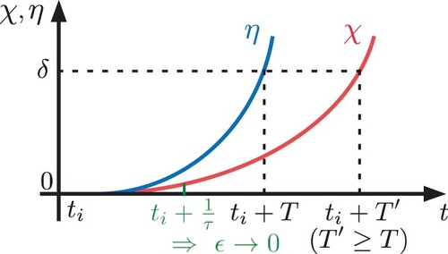Let us now denote $\Vert ϵ\Vert /\Vert e_e\Vert$ by $\chi \ge 0$, i.e. we consider $\dot{\chi }\le 2k_e(1+\chi {)}^2,\chi (t_i)=0,t\in [t_i,t_{i+1})$. Then, if $\eta \left(t\right)$ is the solution of $\dot{\eta }=2k_e(1+\eta {)}^2,\eta (t_i)=0$, we have $\chi \left(t\right)\le \eta \left(t\right)$ for all $t\in [t_i,t_{i+1})$. This means that the time it takes for χ to evolve from 0 to δ is larger than or equal to the time for η (see Figure 4). The time for η is given by $\delta /\left(2k_e\right(1+\delta \left)\right)$ which is obtained by the solution T>0 of $\eta (t_i+T)=\delta$. Therefore, if $1/\tau \le T$ holds, (9(9) $\Vert ϵ\Vert \le \delta \Vert e_e\Vert ,\delta \in (0,1)$(9) ) is guaranteed for all time because ϵ is reset to 0 before $\Vert ϵ\Vert /\Vert e_e\Vert$ reaches to δ (see Figure 4).

Figure 4. Image of time evolution of χ and η.

We finally show the exponential stability of $e_e=0$ after some time, from the Gronwall-Bellman Inequality [24]. Notice that if τ satisfies (7(7) $\tau \ge \frac{2k_e(1+\delta )}{\delta },\delta \in (0,1),$(7) ), then the inequality (10(10) ${\dot{U}}_e\le -k_e(1-\delta )\Vert e_e{\Vert }^2\le 0$(10) ) holds, i.e. ${\dot{U}}_e$ is negative definite for all time. It should be also noted that $U_e$ is continuous and positive definite. Therefore, there exists finite time $T_a>t_0$ in the time sequence $t_i,i\in {\mathbb{N}}_0$ satisfying $U_e\left(t\right)<1{}^{\mathrm{\forall }}t\ge T_a$. Then, $\varphi \left(e^{\hat{\xi }{\theta }_{ee}}\right)<1$ holds for all $t\ge T_a$ from the definition of $U_e$. The property $\varphi \left(e^{\hat{\xi }\theta }\right)\le \Vert \mathrm{s}\mathrm{k}(e^{\hat{\xi }\theta }{)}^{\vee }{\Vert }^2$ also holds for $\varphi \left(e^{\hat{\xi }\theta }\right)<1$.⁴ In summary, (10(10) ${\dot{U}}_e\le -k_e(1-\delta )\Vert e_e{\Vert }^2\le 0$(10) ) provides the following inequality for every interval $t\in [t_i,t_{i+1}),t_i\ge T_a$: ${\dot{U}}_e\left(t\right)\le -k_e(1-\delta )U_e\left(t\right).$Then, from the Gronwall-Bellman Inequality, we obtain (13) $U_e\left(t\right)\le U_e\left(t_i\right)e^{-k_e(1-\delta )(t-t_i)},t\in [t_i,t_{i+1}).$(13) We next consider $t_{i+1}=t_i+1/\tau$. Similarly to the above discussion, we obtain $U_e\left(t\right)\le U_e\left(t_{i+1}\right)e^{-k_e(1-\delta )(t-t_i-1/\tau )},t\in [t_{i+1},t_{i+2}).$Then, since $U_e\left(t_{i+1}\right)\le U_e\left(t_i\right)e^{-k_e(1-\delta )/\tau }$ holds from (13(13) $U_e\left(t\right)\le U_e\left(t_i\right)e^{-k_e(1-\delta )(t-t_i)},t\in [t_i,t_{i+1}).$(13) ) and the continuity of $U_e$, we get $U_e\left(t\right)\le U_e\left(t_i\right)e^{-k_e(1-\delta )(t-t_i)},t\in [t_{i+1},t_{i+2}).$Furthermore, the induction from time $T_a$ gives (14) $U_e\left(t\right)\le U_e\left(T_a\right)e^{-k_e(1-\delta )(t-T_a)\mathrm{\forall }}t\ge T_a.$(14) Finally, we derive the inequality (8(8) $\Vert e_e\left(t\right)\Vert \le {\alpha }_1{e}^{-{\text{β}}_1(t-T_a)\mathrm{\forall }}t\ge T_a$(8) ) from (14(14) $U_e\left(t\right)\le U_e\left(T_a\right)e^{-k_e(1-\delta )(t-T_a)\mathrm{\forall }}t\ge T_a.$(14) ). Remember that $\left(1/2\right)\Vert e_e{\Vert }^2\le U_e\le \Vert e_e{\Vert }^2$ holds after time $T_a$. Then, substituting these inequalities into (14(14) $U_e\left(t\right)\le U_e\left(T_a\right)e^{-k_e(1-\delta )(t-T_a)\mathrm{\forall }}t\ge T_a.$(14) ) yields $\frac{1}{2}\Vert e_e\left(t\right){\Vert }^2\le \Vert e_e\left(T_a\right){\Vert }^2{e}^{-k_e(1-\delta )(t-T_a)\mathrm{\forall }}t\ge T_a.$Therefore, by taking the square root for both sides of this inequality and defining ${\alpha }_1,{\text{β}}_1>0$ as ${\alpha }_1:=\sqrt{2}\Vert e_e\left(T_a\right)\Vert$ and ${\text{β}}_1:=k_e(1-\delta )/2$, we obtain (8(8) $\Vert e_e\left(t\right)\Vert \le {\alpha }_1{e}^{-{\text{β}}_1(t-T_a)\mathrm{\forall }}t\ge T_a$(8) ).

Remark 4.1

The condition (7(7) $\tau \ge \frac{2k_e(1+\delta )}{\delta },\delta \in (0,1),$(7) ) implies that the choice of a large feedback gain $k_e$ requires fast frame rates τ (small sampling intervals). This property is intuitive because large gains increase the influence of the sampling error ϵ, which might be a poor impact on the estimation. In other words, after choosing a camera with a certain frame rate, it is not free to make the gain large. Although the condition (7(7) $\tau \ge \frac{2k_e(1+\delta )}{\delta },\delta \in (0,1),$(7) ) is only sufficient, this analysis provides the significant insight that camera frame rates or image processing time is not negligible for pose estimation.

4.2. Tracking performance analysis

We next analyse the tracking performance for the moving target. Suppose that $\Vert V_{wo}^b\left(t\right)\Vert \le \kappa {}^{\mathrm{\forall }}t\ge t_0$ holds for a positive scalar $\kappa >0$, i.e. the target velocity is bounded. We also assume that the value of κ is known a prior, e.g. simply as prior information or due to hardware limitations of the target vehicle. Then, the time derivative of the potential function $U_e$ along the trajectories of (4(4) ${\dot{g}}_{ee}=-{\hat{u}}_e{g}_{ee}+g_{ee}{\hat{V}}_{wo}^b.$(4) ) and (6(6) $u_e\left(t\right)=k_e{e}_e\left(t_i\right),t\in [t_i,t_{i+1}),k_e>0.$(6) ) yields $\begin{array}{rl}{\dot{U}}_e& =e_e^{\mathrm{T}}{u}_e+e_e^{\mathrm{T}}{\mathrm{A}\mathrm{d}}_{\left(e^{\hat{\xi }{\theta }_{ee}}\right)}{V}_{wo}^b\\ & \le -k_e{e}_e^{\mathrm{T}}{e}_e\left(t_i\right)+\Vert e_e\Vert \Vert V_{wo}^b\Vert \\ & \le -k_e\Vert e_e{\Vert }^2+k_e\Vert e_e\Vert \Vert ϵ\Vert +\kappa \Vert e_e\Vert .\end{array}$Here, for ease of representation, we employ the following notation, differently from ${\mathrm{A}\mathrm{d}}_{\left(g\right)}$ in (5(5) $\begin{array}{rl}& V_{ee}^b:=(g_{ee}^{-1}{\dot{g}}_{ee}{)}^{\vee }=-{\mathrm{A}\mathrm{d}}_{\left(g_{ee}^{-1}\right)}{u}_e+V_{wo}^b,\\ & {\mathrm{A}\mathrm{d}}_{\left(g\right)}:=\left[\begin{array}{cc}{e}^{\hat{\xi }\theta }& \hat{p}{e}^{\hat{\xi }\theta }\\ O_{3\times 3}& e^{\hat{\xi }\theta }\end{array}\right].\end{array}$(5) ): ${\mathrm{A}\mathrm{d}}_{\left(e^{\hat{\xi }\theta }\right)}:=\left[\begin{array}{cc}{e}^{\hat{\xi }\theta }& O_{3\times 3}\\ O_{3\times 3}& e^{\hat{\xi }\theta }\end{array}\right]\in {\mathbb{R}}^{6\times 6}.$ Let us now introduce a performance indicator $\gamma >0$ to evaluate the sampling error ϵ. Then, if $\Vert ϵ\Vert \le \gamma$ is satisfied, we get (15) ${\dot{U}}_e\le -k_e\Vert e_e{\Vert }^2+(k_e\gamma +\kappa )\Vert e_e\Vert .$(15) Since the right-hand side of (15(15) ${\dot{U}}_e\le -k_e\Vert e_e{\Vert }^2+(k_e\gamma +\kappa )\Vert e_e\Vert .$(15) ) consists only of $\Vert e_e\Vert$, we get the following theorem by employing ultimate boundedness analysis [24]:

Theorem 4.2

Suppose that the norm of the target object velocity $V_{wo}^b$ is upper bounded by κ. Then, for every initial estimation error $e_e\left(t_0\right)$, there exists $T_b\ge t_0$ such that the solution $e_e\left(t\right)$ of the closed-loop system (4(4) ${\dot{g}}_{ee}=-{\hat{u}}_e{g}_{ee}+g_{ee}{\hat{V}}_{wo}^b.$(4) ) and (6(6) $u_e\left(t\right)=k_e{e}_e\left(t_i\right),t\in [t_i,t_{i+1}),k_e>0.$(6) ) satisfies (16) $\Vert e_e\left(t\right)\Vert \le \frac{\sqrt{2}(k_e\gamma +\kappa )}{k_e\delta }{}^{\mathrm{\forall }}t\ge T_b$(16) if $|{\theta }_{ee}|\le \pi /2$ and the following frame rate condition hold:

(17) $\tau \ge \{\begin{array}{l}{\displaystyle \frac{k_e}{\ln (1+\frac{k_e\gamma }{2\kappa +2k_e\sqrt{2U_e\left(t_0\right)}})}}\mathrm{i}\mathrm{f}\Vert e_e\left(t_0\right)\Vert \ge {\displaystyle \frac{k_e\gamma +\kappa }{k_e\delta }}\\ {\displaystyle \frac{k_e}{\ln (1+\frac{k_e\gamma \delta }{2\kappa \delta +2\sqrt{2}(k_e\gamma +\kappa )})}}\mathrm{o}\mathrm{t}\mathrm{h}\mathrm{e}\mathrm{r}\mathrm{w}\mathrm{i}\mathrm{s}\mathrm{e}\end{array}.$(17)

Proof.

If $\Vert ϵ\Vert \le \gamma$ is satisfied for all time, we get the following inequality for $\delta \in (0,1)$ from (15(15) ${\dot{U}}_e\le -k_e\Vert e_e{\Vert }^2+(k_e\gamma +\kappa )\Vert e_e\Vert .$(15) ): (18) $\begin{array}{rl}{\dot{U}}_e& \le -k_e(1-\delta )\Vert e_e{\Vert }^2-k_e\delta \Vert e_e{\Vert }^2+(k_e\gamma +\kappa )\Vert e_e\Vert \\ & \le -k_e(1-\delta )\Vert e_e{\Vert }^2{}^{\mathrm{\forall }}\Vert e_e\Vert \ge \frac{k_e\gamma +\kappa }{k_e\delta }.\end{array}$(18) Therefore, from Theorem 4.18 of [24] and the property that $\left(1/2\right)\Vert e_e{\Vert }^2\le U_e\le \Vert e_e{\Vert }^2$ holds for $|{\theta }_{ee}|<\pi /2$, we can conclude that for every $e_e\left(t_0\right)$, there exists $T_b\ge t_0$ such that $e_e\left(t\right)$ satisfies (16(16) $\Vert e_e\left(t\right)\Vert \le \frac{\sqrt{2}(k_e\gamma +\kappa )}{k_e\delta }{}^{\mathrm{\forall }}t\ge T_b$(16) ).

We next derive the frame rate condition to guarantee the inequality $\Vert ϵ\Vert \le \gamma$. Similarly to the proof of Theorem 4.1, we investigate the dynamics of $\Vert ϵ\Vert$ in $t\in [t_i,t_{i+1})$ as follows: (19) $\frac{\mathrm{d}}{\mathrm{d}t}\Vert ϵ\Vert \le \Vert \dot{ϵ}\Vert =\Vert {\dot{e}}_e\Vert \le 2k_e\Vert e_e\left(t_i\right)\Vert +k_e\Vert ϵ\Vert +2\kappa .$(19) The differences from (12(12) $\begin{array}{rl}& \Vert {\dot{e}}_e\Vert \\ & =\Vert \begin{array}{c}-u_{ep}-{\hat{u}}_{eR}{p}_{ee}\\ -{\displaystyle \frac{1}{2}}{e}^{-\hat{\xi }{\theta }_{ee}}\left(\right(1+2\cos {\theta }_{ee})I_3-e^{-\hat{\xi }{\theta }_{ee}})u_{eR}\end{array}\Vert \\ & \le \Vert \begin{array}{c}{k}_e(-I_3-\mathrm{s}\mathrm{k}(e^{\hat{\xi }{\theta }_{ee}\left(t_i\right)}\left)\right)p_{ee}\\ {\displaystyle \frac{k_e}{2}}{e}^{-\hat{\xi }{\theta }_{ee}}(e^{-\hat{\xi }{\theta }_{ee}}-(1+2\cos {\theta }_{ee}\left)I_3\right)\mathrm{s}\mathrm{k}(e^{\hat{\xi }{\theta }_{ee}}{)}^{\vee }\end{array}\Vert \\ & +\Vert \begin{array}{c}{k}_e{ϵ}_p\\ {\displaystyle \frac{k_e}{2}}{e}^{-\hat{\xi }{\theta }_{ee}}(e^{-\hat{\xi }{\theta }_{ee}}-(1+2\cos {\theta }_{ee}\left)I_3\right){ϵ}_R\end{array}\Vert \\ & \le 2k_e\Vert e_e\Vert +2k_e\Vert ϵ\Vert .\end{array}$(12) ) are to handle $V_{wo}^b$ which appears in (4(4) ${\dot{g}}_{ee}=-{\hat{u}}_e{g}_{ee}+g_{ee}{\hat{V}}_{wo}^b.$(4) ) and to consider not $e_e\left(t\right)$ but $e_e\left(t_i\right)$ to reduce the conservativeness. Let us now derive the upper bound of $\Vert e_e\left(t_i\right)\Vert$. We first consider the case that $\Vert e_e\left(t_0\right)\Vert \ge (k_e\gamma +\kappa )/\left(k_e\delta \right)$. Then, the following inequality holds from $\left(1/2\right)\Vert e_e{\Vert }^2\le U_e$ and (18(18) $\begin{array}{rl}{\dot{U}}_e& \le -k_e(1-\delta )\Vert e_e{\Vert }^2-k_e\delta \Vert e_e{\Vert }^2+(k_e\gamma +\kappa )\Vert e_e\Vert \\ & \le -k_e(1-\delta )\Vert e_e{\Vert }^2{}^{\mathrm{\forall }}\Vert e_e\Vert \ge \frac{k_e\gamma +\kappa }{k_e\delta }.\end{array}$(18) ): $\Vert e_e\left(t\right)\Vert \le \sqrt{2U_e\left(t\right)}\le \sqrt{2U_e\left(t_0\right)}{}^{\mathrm{\forall }}t\ge t_0,$which also means $\Vert e_e\left(t_i\right)\Vert \le \sqrt{2U_e\left(t_0\right)}{}^{\mathrm{\forall }}i\in {\mathbb{N}}_0$. We thus obtain $\frac{\mathrm{d}}{\mathrm{d}t}\Vert ϵ\Vert \le k_e\Vert ϵ\Vert +2\kappa +2k_e\sqrt{2U_e\left(t_0\right)}$from (19(19) $\frac{\mathrm{d}}{\mathrm{d}t}\Vert ϵ\Vert \le \Vert \dot{ϵ}\Vert =\Vert {\dot{e}}_e\Vert \le 2k_e\Vert e_e\left(t_i\right)\Vert +k_e\Vert ϵ\Vert +2\kappa .$(19) ) and the first frame rate condition in (17(17) $\tau \ge \{\begin{array}{l}{\displaystyle \frac{k_e}{\ln (1+\frac{k_e\gamma }{2\kappa +2k_e\sqrt{2U_e\left(t_0\right)}})}}\mathrm{i}\mathrm{f}\Vert e_e\left(t_0\right)\Vert \ge {\displaystyle \frac{k_e\gamma +\kappa }{k_e\delta }}\\ {\displaystyle \frac{k_e}{\ln (1+\frac{k_e\gamma \delta }{2\kappa \delta +2\sqrt{2}(k_e\gamma +\kappa )})}}\mathrm{o}\mathrm{t}\mathrm{h}\mathrm{e}\mathrm{r}\mathrm{w}\mathrm{i}\mathrm{s}\mathrm{e}\end{array}.$(17) ) via the same analysis as in Theorem 4.1.

On the other hand, when the initial estimation error satisfies $\Vert e_e\left(t_0\right)\Vert <(k_e\gamma +\kappa )/\left(k_e\delta \right)$, $U_e\left(t\right)$ might increase and become larger than $U_e\left(t_0\right)$. However, since (18(18) $\begin{array}{rl}{\dot{U}}_e& \le -k_e(1-\delta )\Vert e_e{\Vert }^2-k_e\delta \Vert e_e{\Vert }^2+(k_e\gamma +\kappa )\Vert e_e\Vert \\ & \le -k_e(1-\delta )\Vert e_e{\Vert }^2{}^{\mathrm{\forall }}\Vert e_e\Vert \ge \frac{k_e\gamma +\kappa }{k_e\delta }.\end{array}$(18) ) holds, $U_e\left(t\right)$ never goes beyond the value associated with $\Vert e_e\Vert =(k_e\gamma +\kappa )/\left(k_e\delta \right)$, denoted by $U_e^{\ast }$. Then, this fact provides $\Vert e_e\left(t\right)\Vert \le \sqrt{2U_e\left(t\right)}\le \sqrt{2U_e^{\ast }}\le \frac{\sqrt{2}(k_e\gamma +\kappa )}{k_e\delta }{}^{\mathrm{\forall }}t\ge t_0$for $|{\theta }_{ee}|<\pi /2$. Therefore, we obtain $\frac{\mathrm{d}}{\mathrm{d}t}\Vert ϵ\Vert \le k_e\Vert ϵ\Vert +2\kappa +\frac{2\sqrt{2}(k_e\gamma +\kappa )}{\delta }$from (19(19) $\frac{\mathrm{d}}{\mathrm{d}t}\Vert ϵ\Vert \le \Vert \dot{ϵ}\Vert =\Vert {\dot{e}}_e\Vert \le 2k_e\Vert e_e\left(t_i\right)\Vert +k_e\Vert ϵ\Vert +2\kappa .$(19) ) and the second frame rate condition in (17(17) $\tau \ge \{\begin{array}{l}{\displaystyle \frac{k_e}{\ln (1+\frac{k_e\gamma }{2\kappa +2k_e\sqrt{2U_e\left(t_0\right)}})}}\mathrm{i}\mathrm{f}\Vert e_e\left(t_0\right)\Vert \ge {\displaystyle \frac{k_e\gamma +\kappa }{k_e\delta }}\\ {\displaystyle \frac{k_e}{\ln (1+\frac{k_e\gamma \delta }{2\kappa \delta +2\sqrt{2}(k_e\gamma +\kappa )})}}\mathrm{o}\mathrm{t}\mathrm{h}\mathrm{e}\mathrm{r}\mathrm{w}\mathrm{i}\mathrm{s}\mathrm{e}\end{array}.$(17) ).

Remark 4.2

The performance evaluation (16(16) $\Vert e_e\left(t\right)\Vert \le \frac{\sqrt{2}(k_e\gamma +\kappa )}{k_e\delta }{}^{\mathrm{\forall }}t\ge T_b$(16) ) can be rewritten as follows: $\Vert e_e\left(t\right)\Vert \le \frac{\sqrt{2}\gamma }{\delta }+\frac{\sqrt{2}\kappa }{k_e\delta }{}^{\mathrm{\forall }}t\ge T_b.$This means that smaller γ and larger $k_e$ achieve better performance. However, both of them require fast frame rates because the right-hand sides of (17(17) $\tau \ge \{\begin{array}{l}{\displaystyle \frac{k_e}{\ln (1+\frac{k_e\gamma }{2\kappa +2k_e\sqrt{2U_e\left(t_0\right)}})}}\mathrm{i}\mathrm{f}\Vert e_e\left(t_0\right)\Vert \ge {\displaystyle \frac{k_e\gamma +\kappa }{k_e\delta }}\\ {\displaystyle \frac{k_e}{\ln (1+\frac{k_e\gamma \delta }{2\kappa \delta +2\sqrt{2}(k_e\gamma +\kappa )})}}\mathrm{o}\mathrm{t}\mathrm{h}\mathrm{e}\mathrm{r}\mathrm{w}\mathrm{i}\mathrm{s}\mathrm{e}\end{array}.$(17) ) are monotonically decreasing for γ and monotonically increasing for $k_e$. Therefore, as we expected, γ can be considered as the indicator of the tracking performance and the (sufficiently) allowable gains for a designer. For example, choosing a camera with a certain rate enables us to design $k_e$ for desired performance related to γ from (16(16) $\Vert e_e\left(t\right)\Vert \le \frac{\sqrt{2}(k_e\gamma +\kappa )}{k_e\delta }{}^{\mathrm{\forall }}t\ge T_b$(16) ) and (17(17) $\tau \ge \{\begin{array}{l}{\displaystyle \frac{k_e}{\ln (1+\frac{k_e\gamma }{2\kappa +2k_e\sqrt{2U_e\left(t_0\right)}})}}\mathrm{i}\mathrm{f}\Vert e_e\left(t_0\right)\Vert \ge {\displaystyle \frac{k_e\gamma +\kappa }{k_e\delta }}\\ {\displaystyle \frac{k_e}{\ln (1+\frac{k_e\gamma \delta }{2\kappa \delta +2\sqrt{2}(k_e\gamma +\kappa )})}}\mathrm{o}\mathrm{t}\mathrm{h}\mathrm{e}\mathrm{r}\mathrm{w}\mathrm{i}\mathrm{s}\mathrm{e}\end{array}.$(17) ). A design example is provided in Section 7.

Remark 4.3

Theorem 4.2 provides two frame rate conditions depending on the initial estimation error. However, if we first run the present estimation law (6(6) $u_e\left(t\right)=k_e{e}_e\left(t_i\right),t\in [t_i,t_{i+1}),k_e>0.$(6) ) before the target moves, we can consider only the second condition.

5. Sampled visual feedback pose regulation

We next propose a sampled visual feedback pose regulation mechanism based on the present sampled visual motion observer for the objective (ii).

5.1. Control error system

Similarly to the estimation error system (4(4) ${\dot{g}}_{ee}=-{\hat{u}}_e{g}_{ee}+g_{ee}{\hat{V}}_{wo}^b.$(4) ) presented in Section 3.1, we build the control error system. The control error $g_{ce}=(p_{ce},e^{\hat{\xi }{\theta }_{ce}})\in SE\left(3\right)$, and its vector form $e_c\in {\mathbb{R}}^6$ are defined as follows: $g_{ce}:=g_d^{-1}{\overline{g}}_{co},e_c:=\left[\begin{array}{c}{p}_{ce}\\ \mathrm{s}\mathrm{k}(e^{\hat{\xi }{\theta }_{ce}}{)}^{\vee }\end{array}\right].$Notice that for ${\theta }_{ce}\in (-\pi ,\pi )$, $e_c=0$ holds if and only if $g_{ce}=I_4$, i.e. ${\overline{g}}_{co}=g_d$. Then, the time derivative of $g_{ce}$ along the trajectories of (3(3) ${\dot{\overline{g}}}_{co}=-{\hat{V}}_{wc}^b{\overline{g}}_{co}+{\overline{g}}_{co}{\hat{u}}_e.$(3) ) provides the following control error system: (20) ${\dot{g}}_{ce}=-g_d^{-1}{\hat{V}}_{wc}^b{g}_d{g}_{ce}+g_{ce}{\hat{u}}_e.$(20) This is also written in the vector form as $V_{ce}^b:=(g_{ce}^{-1}{\dot{g}}_{ce}{)}^{\vee }=-{\mathrm{A}\mathrm{d}}_{\left(g_{ce}^{-1}\right)}{\mathrm{A}\mathrm{d}}_{\left(g_d^{-1}\right)}{V}_{wc}^b+u_e.$Combining the estimation error system (4(4) ${\dot{g}}_{ee}=-{\hat{u}}_e{g}_{ee}+g_{ee}{\hat{V}}_{wo}^b.$(4) ) with the control error system (20(20) ${\dot{g}}_{ce}=-g_d^{-1}{\hat{V}}_{wc}^b{g}_d{g}_{ce}+g_{ce}{\hat{u}}_e.$(20) ) yields the following total error system in the vector form: (21) $\begin{array}{rl}& \left[\begin{array}{c}{V}_{ce}^b\\ V_{ee}^b\end{array}\right]=-\left[\begin{array}{cc}{\mathrm{A}\mathrm{d}}_{\left(g_{ce}^{-1}\right)}& -I_6\\ O_{6\times 6}& {\mathrm{A}\mathrm{d}}_{\left(g_{ee}^{-1}\right)}\end{array}\right]u_{ce}+\left[\begin{array}{c}0\\ V_{wo}^b\end{array}\right],\\ & u_{ce}:=\left[\begin{array}{c}{\mathrm{A}\mathrm{d}}_{\left(g_d^{-1}\right)}{V}_{wc}^b\\ u_e\end{array}\right]\in {\mathbb{R}}^{12}.\end{array}$(21) It is shown in [13] that if $V_{wo}^b=0$, the total error system (21(21) $\begin{array}{rl}& \left[\begin{array}{c}{V}_{ce}^b\\ V_{ee}^b\end{array}\right]=-\left[\begin{array}{cc}{\mathrm{A}\mathrm{d}}_{\left(g_{ce}^{-1}\right)}& -I_6\\ O_{6\times 6}& {\mathrm{A}\mathrm{d}}_{\left(g_{ee}^{-1}\right)}\end{array}\right]u_{ce}+\left[\begin{array}{c}0\\ V_{wo}^b\end{array}\right],\\ & u_{ce}:=\left[\begin{array}{c}{\mathrm{A}\mathrm{d}}_{\left(g_d^{-1}\right)}{V}_{wc}^b\\ u_e\end{array}\right]\in {\mathbb{R}}^{12}.\end{array}$(21) ) also has a passivity-like property from the input $u_{ce}$ to the output ${\nu }_{ce}\in {\mathbb{R}}^{12}$ defined as $\begin{array}{rl}& {\nu }_{ce}:=N{e}_{ce},N:=\left[\begin{array}{cc}-I_6& O_{6\times 6}\\ {\mathrm{A}\mathrm{d}}_{\left(e^{-\hat{\xi }{\theta }_{ce}}\right)}& -I_6\end{array}\right]\in {\mathbb{R}}^{12\times 12},\\ & e_{ce}:=\left[\begin{array}{c}{e}_c\\ e_e\end{array}\right]\in {\mathbb{R}}^{12}.\end{array}$Here, $e_{ce}$ is the total control and estimation error vector, and the corresponding storage function $U\ge 0$ is defined as $U:=\frac{1}{2}\Vert p_{ce}{\Vert }^2+\varphi \left(e^{\hat{\xi }{\theta }_{ce}}\right)+\frac{1}{2}\Vert p_{ee}{\Vert }^2+\varphi \left(e^{\hat{\xi }{\theta }_{ee}}\right),$which yields $\dot{U}=u_{ce}^{\mathrm{T}}{\nu }_{ce}$, i.e. a passivity-like property from the input $u_{ce}$ to the output ${\nu }_{ce}$ [13]. We note that U=0 is equivalent to $e_{ce}=0$ for ${\theta }_{ce},{\theta }_{ee}\in (-\pi ,\pi )$, and $e_{ce}=0$ means $g_{co}=g_d$, that is, the pose regulation (the objective (ii)) is achieved.

Based on the passivity-like property, Fujita et al. [13] propose the following negative feedback law to achieve the pose regulation as in Figure 1(a): $u_{ce}=-K{\nu }_{ce},K>0.$Here, $K\in {\mathbb{R}}^{12\times 12}$ is a positive definite gain matrix, and the achievement of the regulation is proved by the direct use of the storage function U as a potential function for the Lyapunov-based energy approach. However, this technique also assumes the continuous availability of the visual measurements f, which allows any positive definite matrix K.

5.2. Pose regulation mechanism

Consider the same settings as in Section 3, i.e. the fixed frame rate τ and the sampling time sequence $t_i,i\in {\mathbb{N}}_0$. Then, motivated by the passivity-like property of the total error system (21(21) $\begin{array}{rl}& \left[\begin{array}{c}{V}_{ce}^b\\ V_{ee}^b\end{array}\right]=-\left[\begin{array}{cc}{\mathrm{A}\mathrm{d}}_{\left(g_{ce}^{-1}\right)}& -I_6\\ O_{6\times 6}& {\mathrm{A}\mathrm{d}}_{\left(g_{ee}^{-1}\right)}\end{array}\right]u_{ce}+\left[\begin{array}{c}0\\ V_{wo}^b\end{array}\right],\\ & u_{ce}:=\left[\begin{array}{c}{\mathrm{A}\mathrm{d}}_{\left(g_d^{-1}\right)}{V}_{wc}^b\\ u_e\end{array}\right]\in {\mathbb{R}}^{12}.\end{array}$(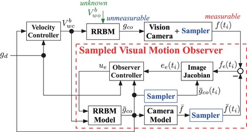21) ), we propose the following visual feedback pose regulation input based on the sampled visual motion observer: (22) $\begin{array}{rl}{u}_{ce}\left(t\right)& =K\left[\begin{array}{c}{e}_c\left(t\right)\\ e_e\left(t_i\right)-{\mathrm{A}\mathrm{d}}_{\left(e^{-\hat{\xi }{\theta }_{ce}}\right)}{e}_c\left(t\right)\end{array}\right],t\in [t_i,t_{i+1}),\\ K& :=\left[\begin{array}{cc}{k}_c{I}_6& O_{6\times 6}\\ O_{6\times 6}& k_e{I}_6\end{array}\right]\in {\mathbb{R}}^{12\times 12},k_c,k_e>0.\end{array}$(22) Notice here that only the estimation error $e_e\left(t_i\right)$ is constant until the next sampling time since we consider the case that the computation time to obtain the estimate ${\overline{g}}_{co}$ is small enough to be neglected. This structure enables us to greatly reduce the conservativeness of the frame rate condition provided by the conference version of this paper [22]. In [22], ${\overline{g}}_{co}$ is also sampled, i.e. instead of $e_c\left(t\right)$ and $e^{-\hat{\xi }{\theta }_{ce}\left(t\right)}$, $e_c\left(t_i\right)$ and $e^{-\hat{\xi }{\theta }_{ce}\left(t_i\right)}$ are used in the regulation input (22(22) $\begin{array}{rl}{u}_{ce}\left(t\right)& =K\left[\begin{array}{c}{e}_c\left(t\right)\\ e_e\left(t_i\right)-{\mathrm{A}\mathrm{d}}_{\left(e^{-\hat{\xi }{\theta }_{ce}}\right)}{e}_c\left(t\right)\end{array}\right],t\in [t_i,t_{i+1}),\\ K& :=\left[\begin{array}{cc}{k}_c{I}_6& O_{6\times 6}\\ O_{6\times 6}& k_e{I}_6\end{array}\right]\in {\mathbb{R}}^{12\times 12},k_c,k_e>0.\end{array}$(22) ).

This paper assumes $k_e\le k_c$ for better performance in the subsequent discussion. The reason to employ this gain relationship is that only the observer input for the estimation is sampled, and as a result, a large gain $k_e$ increases the influence of the sampling error $ϵ\left(t\right)=e_e\left(t\right)-e_e\left(t_i\right)$, which results in bad control performance. The block diagram of the present sampled visual feedback system is illustrated in Figure 5.

Figure 5. Block diagram of sampled visual feedback system.

6. Analysis of pose regulation

Similarly to Section 4, this section provides the convergence analysis for the stationary target object and the tracking performance analysis for the moving target.

6.1. Convergence analysis

Using the same definition of the sampling error $ϵ\left(t\right)=e_e\left(t\right)-e_e\left(t_i\right),t\in [t_i,t_{i+1}){}^{\mathrm{\forall }}i\in {\mathbb{N}}_0$ as in Section 4, we have the following theorem:

Theorem 6.1

Suppose that the target object is static (i.e. $V_{wo}^b\equiv 0$). Then, if the camera frame rate satisfies the condition

(23) $\begin{array}{rl}& \tau \ge \frac{\sqrt{(k_c+4k_e+\sqrt{k_c^2+4k_e^2}{)}^2-16\sqrt{5}{k}_e^2}}{\ln \left(\frac{\begin{array}{c}8\sqrt{5}{k}_e+(3-\sqrt{5})\delta (k_c+4k_e+\sqrt{k_c^2+4k_e^2})\\ +\sqrt{(k_c+4k_e+\sqrt{k_c^2+4k_e^2}{)}^2-16\sqrt{5}{k}_e^2}\end{array}}{\begin{array}{c}8\sqrt{5}{k}_e+(3-\sqrt{5})\delta (k_c+4k_e+\sqrt{k_c^2+4k_e^2})\\ -\sqrt{(k_c+4k_e+\sqrt{k_c^2+4k_e^2}{)}^2-16\sqrt{5}{k}_e^2}\end{array}}\right)},\\ & \delta \in (0,1),\end{array}$(23) there exist finite time $T_c\ge t_0$ and positive scalars ${\alpha }_2,{\text{β}}_2>0$ such that $\Vert e_{ce}\left(t\right)\Vert \le {\alpha }_2{e}^{-{\text{β}}_2(t-T_c)\mathrm{\forall }}t\ge T_c$for the closed-loop system (21(21) $\begin{array}{rl}& \left[\begin{array}{c}{V}_{ce}^b\\ V_{ee}^b\end{array}\right]=-\left[\begin{array}{cc}{\mathrm{A}\mathrm{d}}_{\left(g_{ce}^{-1}\right)}& -I_6\\ O_{6\times 6}& {\mathrm{A}\mathrm{d}}_{\left(g_{ee}^{-1}\right)}\end{array}\right]u_{ce}+\left[\begin{array}{c}0\\ V_{wo}^b\end{array}\right],\\ & u_{ce}:=\left[\begin{array}{c}{\mathrm{A}\mathrm{d}}_{\left(g_d^{-1}\right)}{V}_{wc}^b\\ u_e\end{array}\right]\in {\mathbb{R}}^{12}.\end{array}$(21) ) and (22(22) $\begin{array}{rl}{u}_{ce}\left(t\right)& =K\left[\begin{array}{c}{e}_c\left(t\right)\\ e_e\left(t_i\right)-{\mathrm{A}\mathrm{d}}_{\left(e^{-\hat{\xi }{\theta }_{ce}}\right)}{e}_c\left(t\right)\end{array}\right],t\in [t_i,t_{i+1}),\\ K& :=\left[\begin{array}{cc}{k}_c{I}_6& O_{6\times 6}\\ O_{6\times 6}& k_e{I}_6\end{array}\right]\in {\mathbb{R}}^{12\times 12},k_c,k_e>0.\end{array}$(22) ).

Proof.

When $V_{wo}^b=0$ holds, the time derivative of the potential function U along the trajectories of (21(21) $\begin{array}{rl}& \left[\begin{array}{c}{V}_{ce}^b\\ V_{ee}^b\end{array}\right]=-\left[\begin{array}{cc}{\mathrm{A}\mathrm{d}}_{\left(g_{ce}^{-1}\right)}& -I_6\\ O_{6\times 6}& {\mathrm{A}\mathrm{d}}_{\left(g_{ee}^{-1}\right)}\end{array}\right]u_{ce}+\left[\begin{array}{c}0\\ V_{wo}^b\end{array}\right],\\ & u_{ce}:=\left[\begin{array}{c}{\mathrm{A}\mathrm{d}}_{\left(g_d^{-1}\right)}{V}_{wc}^b\\ u_e\end{array}\right]\in {\mathbb{R}}^{12}.\end{array}$(21) ) and (22(22) $\begin{array}{rl}{u}_{ce}\left(t\right)& =K\left[\begin{array}{c}{e}_c\left(t\right)\\ e_e\left(t_i\right)-{\mathrm{A}\mathrm{d}}_{\left(e^{-\hat{\xi }{\theta }_{ce}}\right)}{e}_c\left(t\right)\end{array}\right],t\in [t_i,t_{i+1}),\\ K& :=\left[\begin{array}{cc}{k}_c{I}_6& O_{6\times 6}\\ O_{6\times 6}& k_e{I}_6\end{array}\right]\in {\mathbb{R}}^{12\times 12},k_c,k_e>0.\end{array}$(22) ) for $t\in [t_i,t_{i+1})$ yields $\begin{array}{rl}\dot{U}& =e_{ce}^{\mathrm{T}}{N}^{\mathrm{T}}{u}_{ce}\\ & =-e_{ce}^{\mathrm{T}}{N}^{\mathrm{T}}KN{e}_{ce}+k_e(e_c^{\mathrm{T}}-e_c^{\mathrm{T}}{\mathrm{A}\mathrm{d}}_{\left(e^{\hat{\xi }{\theta }_{ce}}\right)})ϵ\\ & \le -\frac{3-\sqrt{5}}{2}{k}_e\Vert e_{ce}{\Vert }^2+\sqrt{2}{k}_e\Vert e_{ce}\Vert \Vert ϵ\Vert .\end{array}$Here, we use the property $e_{ce}^{\mathrm{T}}{N}^{\mathrm{T}}KN{e}_{ce}\ge {\lambda }_{min}\left(N^{\mathrm{T}}KN\right)\Vert e_{ce}{\Vert }^2=(3-\sqrt{5})k_e\Vert e_{ce}{\Vert }^2/2$. (${\lambda }_{min}\left(A\right)\in \mathbb{R}$ is the smallest eigenvalue for any symmetric matrix $A\in {\mathbb{R}}^{n\times n}$.) Therefore, if the inequality $\Vert ϵ\Vert \le \frac{(3-\sqrt{5})}{2\sqrt{2}}\delta \Vert e_{ce}\Vert$is satisfied, we obtain $\dot{U}\le -\frac{3-\sqrt{5}}{2}{k}_e(1-\delta )\Vert e_{ce}{\Vert }^2$for $t\in [t_i,t_{i+1})$.

Then, by the same techniques as in the proof of Theorem 4.1, we get (24) $\frac{\mathrm{d}}{\mathrm{d}t}\frac{\Vert ϵ\Vert }{\Vert e_{ce}\Vert }\le \frac{\Vert {\dot{e}}_e\Vert }{\Vert e_{ce}\Vert }+\frac{\Vert ϵ\Vert }{\Vert e_{ce}{\Vert }^2}\Vert {\dot{e}}_{ce}\Vert$(24) and (25) $\begin{array}{rl}& \Vert {\dot{e}}_e\Vert \le \sqrt{10}{k}_e\Vert e_{ce}\Vert +2k_e\Vert ϵ\Vert ,\\ & \Vert {\dot{e}}_{ce}\Vert \le (k_c+2k_e+\sqrt{k_c^2+4k_e^2})\Vert e_{ce}\Vert +2\sqrt{2}{k}_e\Vert ϵ\Vert .\end{array}$(25) Substituting (25(25) $\begin{array}{rl}& \Vert {\dot{e}}_e\Vert \le \sqrt{10}{k}_e\Vert e_{ce}\Vert +2k_e\Vert ϵ\Vert ,\\ & \Vert {\dot{e}}_{ce}\Vert \le (k_c+2k_e+\sqrt{k_c^2+4k_e^2})\Vert e_{ce}\Vert +2\sqrt{2}{k}_e\Vert ϵ\Vert .\end{array}$(25) ) into (24(24) $\frac{\mathrm{d}}{\mathrm{d}t}\frac{\Vert ϵ\Vert }{\Vert e_{ce}\Vert }\le \frac{\Vert {\dot{e}}_e\Vert }{\Vert e_{ce}\Vert }+\frac{\Vert ϵ\Vert }{\Vert e_{ce}{\Vert }^2}\Vert {\dot{e}}_{ce}\Vert$(24) ) provides $\begin{array}{rl}\frac{\mathrm{d}}{\mathrm{d}t}\frac{\Vert ϵ\Vert }{\Vert e_{ce}\Vert }& \le 2\sqrt{2}{k}_e{\left(\frac{\Vert ϵ\Vert }{\Vert e_{ce}\Vert }\right)}^2\\ & +(k_c+4k_e+\sqrt{k_c^2+4k_e^2})\frac{\Vert ϵ\Vert }{\Vert e_{ce}\Vert }+\sqrt{10}{k}_e.\end{array}$The remaining analysis to obtain the frame rate condition (23(23) $\begin{array}{rl}& \tau \ge \frac{\sqrt{(k_c+4k_e+\sqrt{k_c^2+4k_e^2}{)}^2-16\sqrt{5}{k}_e^2}}{\ln \left(\frac{\begin{array}{c}8\sqrt{5}{k}_e+(3-\sqrt{5})\delta (k_c+4k_e+\sqrt{k_c^2+4k_e^2})\\ +\sqrt{(k_c+4k_e+\sqrt{k_c^2+4k_e^2}{)}^2-16\sqrt{5}{k}_e^2}\end{array}}{\begin{array}{c}8\sqrt{5}{k}_e+(3-\sqrt{5})\delta (k_c+4k_e+\sqrt{k_c^2+4k_e^2})\\ -\sqrt{(k_c+4k_e+\sqrt{k_c^2+4k_e^2}{)}^2-16\sqrt{5}{k}_e^2}\end{array}}\right)},\\ & \delta \in (0,1),\end{array}$(23) ) is the same as in the proof of Theorem 4.1

The condition (23(23) $\begin{array}{rl}& \tau \ge \frac{\sqrt{(k_c+4k_e+\sqrt{k_c^2+4k_e^2}{)}^2-16\sqrt{5}{k}_e^2}}{\ln \left(\frac{\begin{array}{c}8\sqrt{5}{k}_e+(3-\sqrt{5})\delta (k_c+4k_e+\sqrt{k_c^2+4k_e^2})\\ +\sqrt{(k_c+4k_e+\sqrt{k_c^2+4k_e^2}{)}^2-16\sqrt{5}{k}_e^2}\end{array}}{\begin{array}{c}8\sqrt{5}{k}_e+(3-\sqrt{5})\delta (k_c+4k_e+\sqrt{k_c^2+4k_e^2})\\ -\sqrt{(k_c+4k_e+\sqrt{k_c^2+4k_e^2}{)}^2-16\sqrt{5}{k}_e^2}\end{array}}\right)},\\ & \delta \in (0,1),\end{array}$(23) ) also implies that large feedback gains $k_c$ and $k_e$ require fast camera frame rates τ.

6.2. Tracking performance analysis

By using the same assumption $\Vert V_{wo}^b\Vert \le \kappa {}^{\mathrm{\forall }}t\ge t_0$ as in Section 4.2, the time derivative of the potential function U along the trajectories of (21(21) $\begin{array}{rl}& \left[\begin{array}{c}{V}_{ce}^b\\ V_{ee}^b\end{array}\right]=-\left[\begin{array}{cc}{\mathrm{A}\mathrm{d}}_{\left(g_{ce}^{-1}\right)}& -I_6\\ O_{6\times 6}& {\mathrm{A}\mathrm{d}}_{\left(g_{ee}^{-1}\right)}\end{array}\right]u_{ce}+\left[\begin{array}{c}0\\ V_{wo}^b\end{array}\right],\\ & u_{ce}:=\left[\begin{array}{c}{\mathrm{A}\mathrm{d}}_{\left(g_d^{-1}\right)}{V}_{wc}^b\\ u_e\end{array}\right]\in {\mathbb{R}}^{12}.\end{array}$(21) ) and (22(22) $\begin{array}{rl}{u}_{ce}\left(t\right)& =K\left[\begin{array}{c}{e}_c\left(t\right)\\ e_e\left(t_i\right)-{\mathrm{A}\mathrm{d}}_{\left(e^{-\hat{\xi }{\theta }_{ce}}\right)}{e}_c\left(t\right)\end{array}\right],t\in [t_i,t_{i+1}),\\ K& :=\left[\begin{array}{cc}{k}_c{I}_6& O_{6\times 6}\\ O_{6\times 6}& k_e{I}_6\end{array}\right]\in {\mathbb{R}}^{12\times 12},k_c,k_e>0.\end{array}$(22) ) is given as follows: $\begin{array}{rl}\dot{U}& =e_{ce}^{\mathrm{T}}{N}^{\mathrm{T}}{u}_{ce}+e_e^{\mathrm{T}}{\mathrm{A}\mathrm{d}}_{\left(e^{\hat{\xi }{\theta }_{ee}}\right)}{V}_{wo}^b\\ & \le -\frac{3-\sqrt{5}}{2}{k}_e\Vert e_{ce}{\Vert }^2+\sqrt{2}{k}_e\Vert e_{ce}\Vert \Vert ϵ\Vert +\kappa \Vert e_{ce}\Vert .\end{array}$Here, we note that $V_{wo}^b$ appears only in the estimation part for the total error system (21(21) $\begin{array}{rl}& \left[\begin{array}{c}{V}_{ce}^b\\ V_{ee}^b\end{array}\right]=-\left[\begin{array}{cc}{\mathrm{A}\mathrm{d}}_{\left(g_{ce}^{-1}\right)}& -I_6\\ O_{6\times 6}& {\mathrm{A}\mathrm{d}}_{\left(g_{ee}^{-1}\right)}\end{array}\right]u_{ce}+\left[\begin{array}{c}0\\ V_{wo}^b\end{array}\right],\\ & u_{ce}:=\left[\begin{array}{c}{\mathrm{A}\mathrm{d}}_{\left(g_d^{-1}\right)}{V}_{wc}^b\\ u_e\end{array}\right]\in {\mathbb{R}}^{12}.\end{array}$(21) ). Therefore, if $\Vert ϵ\Vert \le \gamma$ is satisfied for a certain performance indicator $\gamma >0$, we get (26) $\dot{U}\le -\frac{3-\sqrt{5}}{2}{k}_e\Vert e_{ce}{\Vert }^2+(\sqrt{2}{k}_e\gamma +\kappa )\Vert e_{ce}\Vert .$(26) Then, we have the following theorem similar to Theorem 4.2:

Theorem 6.2

Suppose that the norm of the target object velocity $V_{wo}^b$ is upper bounded by κ. Then, for every initial control and estimation error $e_{ce}\left(t_0\right)$, there exists $T_d\ge t_0$ such that the solution $e_{ce}\left(t\right)$ of the closed-loop system (21(21) $\begin{array}{rl}& \left[\begin{array}{c}{V}_{ce}^b\\ V_{ee}^b\end{array}\right]=-\left[\begin{array}{cc}{\mathrm{A}\mathrm{d}}_{\left(g_{ce}^{-1}\right)}& -I_6\\ O_{6\times 6}& {\mathrm{A}\mathrm{d}}_{\left(g_{ee}^{-1}\right)}\end{array}\right]u_{ce}+\left[\begin{array}{c}0\\ V_{wo}^b\end{array}\right],\\ & u_{ce}:=\left[\begin{array}{c}{\mathrm{A}\mathrm{d}}_{\left(g_d^{-1}\right)}{V}_{wc}^b\\ u_e\end{array}\right]\in {\mathbb{R}}^{12}.\end{array}$(21) ) and (22(22) $\begin{array}{rl}{u}_{ce}\left(t\right)& =K\left[\begin{array}{c}{e}_c\left(t\right)\\ e_e\left(t_i\right)-{\mathrm{A}\mathrm{d}}_{\left(e^{-\hat{\xi }{\theta }_{ce}}\right)}{e}_c\left(t\right)\end{array}\right],t\in [t_i,t_{i+1}),\\ K& :=\left[\begin{array}{cc}{k}_c{I}_6& O_{6\times 6}\\ O_{6\times 6}& k_e{I}_6\end{array}\right]\in {\mathbb{R}}^{12\times 12},k_c,k_e>0.\end{array}$(22) ) satisfies (27) $\Vert e_{ce}\left(t\right)\Vert \le \frac{4k_e\gamma +2\sqrt{2}\kappa }{(3-\sqrt{5})k_e\delta }{}^{\mathrm{\forall }}t\ge T_d$(27) if $|{\theta }_{ee}|,|{\theta }_{ce}|\le \pi /2$ and the following frame rate condition hold:

(28) $\tau \ge \{\begin{array}{l}{\displaystyle \frac{2k_e}{\ln (1+\frac{k_e\gamma }{\kappa +k_e\sqrt{5U\left(t_0\right)}})}}\mathrm{i}\mathrm{f}\Vert e_{ce}\left(t_0\right)\Vert \ge {\displaystyle \frac{2(\sqrt{2}{k}_e\gamma +\kappa )}{(3-\sqrt{5})k_e\delta }}\\ {\displaystyle \frac{2k_e}{\ln (1+\frac{(6-2\sqrt{5})k_e\gamma \delta }{(6-2\sqrt{5})\kappa \delta +4\sqrt{5}(\sqrt{2}{k}_e\gamma +\kappa )})}}\mathrm{o}\mathrm{t}\mathrm{h}\mathrm{e}\mathrm{r}\mathrm{w}\mathrm{i}\mathrm{s}\mathrm{e}\end{array}.$(28)

Proof.

If $\Vert ϵ\Vert \le \gamma$ is satisfied for all time, the following inequality is obtained from (26(26) $\dot{U}\le -\frac{3-\sqrt{5}}{2}{k}_e\Vert e_{ce}{\Vert }^2+(\sqrt{2}{k}_e\gamma +\kappa )\Vert e_{ce}\Vert .$(26) ): $\begin{array}{rl}\dot{U}& \le -\frac{3-\sqrt{5}}{2}{k}_e(1-\delta )\Vert e_{ce}{\Vert }^2\mathrm{\forall }\Vert e_{ce}\Vert \\ & \ge \frac{2(\sqrt{2}{k}_e\gamma +\kappa )}{(3-\sqrt{5})k_e\delta },\delta \in (0,1).\end{array}$Therefore, from Theorem 4.18 of [24] and the property that $\left(1/2\right)\Vert e_{ce}{\Vert }^2\le U\le \Vert e_{ce}{\Vert }^2$ holds for $|{\theta }_{ee}|,|{\theta }_{ce}|<\pi /2$, we can conclude that for every $e_{ce}\left(t_0\right)$, there exists $T_d\ge t_0$ such that $e_{ce}\left(t\right)$ satisfies (27(27) $\Vert e_{ce}\left(t\right)\Vert \le \frac{4k_e\gamma +2\sqrt{2}\kappa }{(3-\sqrt{5})k_e\delta }{}^{\mathrm{\forall }}t\ge T_d$(27) ).

We next derive the frame rate condition to guarantee the inequality $\Vert ϵ\Vert \le \gamma$. We get the following dynamics of $\Vert ϵ\Vert$ from (21(21) $\begin{array}{rl}& \left[\begin{array}{c}{V}_{ce}^b\\ V_{ee}^b\end{array}\right]=-\left[\begin{array}{cc}{\mathrm{A}\mathrm{d}}_{\left(g_{ce}^{-1}\right)}& -I_6\\ O_{6\times 6}& {\mathrm{A}\mathrm{d}}_{\left(g_{ee}^{-1}\right)}\end{array}\right]u_{ce}+\left[\begin{array}{c}0\\ V_{wo}^b\end{array}\right],\\ & u_{ce}:=\left[\begin{array}{c}{\mathrm{A}\mathrm{d}}_{\left(g_d^{-1}\right)}{V}_{wc}^b\\ u_e\end{array}\right]\in {\mathbb{R}}^{12}.\end{array}$(21) ) and (25(25) $\begin{array}{rl}& \Vert {\dot{e}}_e\Vert \le \sqrt{10}{k}_e\Vert e_{ce}\Vert +2k_e\Vert ϵ\Vert ,\\ & \Vert {\dot{e}}_{ce}\Vert \le (k_c+2k_e+\sqrt{k_c^2+4k_e^2})\Vert e_{ce}\Vert +2\sqrt{2}{k}_e\Vert ϵ\Vert .\end{array}$(25) ): $\frac{\mathrm{d}}{\mathrm{d}t}\Vert ϵ\Vert \le \Vert \dot{ϵ}\Vert =\Vert {\dot{e}}_e\Vert \le \sqrt{10}{k}_e\Vert e_{ce}\Vert +2k_e\Vert ϵ\Vert +2\kappa .$Then, by the same approach as in the proof of Theorem 4.2, we get the frame rate condition (28(28) $\tau \ge \{\begin{array}{l}{\displaystyle \frac{2k_e}{\ln (1+\frac{k_e\gamma }{\kappa +k_e\sqrt{5U\left(t_0\right)}})}}\mathrm{i}\mathrm{f}\Vert e_{ce}\left(t_0\right)\Vert \ge {\displaystyle \frac{2(\sqrt{2}{k}_e\gamma +\kappa )}{(3-\sqrt{5})k_e\delta }}\\ {\displaystyle \frac{2k_e}{\ln (1+\frac{(6-2\sqrt{5})k_e\gamma \delta }{(6-2\sqrt{5})\kappa \delta +4\sqrt{5}(\sqrt{2}{k}_e\gamma +\kappa )})}}\mathrm{o}\mathrm{t}\mathrm{h}\mathrm{e}\mathrm{r}\mathrm{w}\mathrm{i}\mathrm{s}\mathrm{e}\end{array}.$(28) ).

The condition (28(28) $\tau \ge \{\begin{array}{l}{\displaystyle \frac{2k_e}{\ln (1+\frac{k_e\gamma }{\kappa +k_e\sqrt{5U\left(t_0\right)}})}}\mathrm{i}\mathrm{f}\Vert e_{ce}\left(t_0\right)\Vert \ge {\displaystyle \frac{2(\sqrt{2}{k}_e\gamma +\kappa )}{(3-\sqrt{5})k_e\delta }}\\ {\displaystyle \frac{2k_e}{\ln (1+\frac{(6-2\sqrt{5})k_e\gamma \delta }{(6-2\sqrt{5})\kappa \delta +4\sqrt{5}(\sqrt{2}{k}_e\gamma +\kappa )})}}\mathrm{o}\mathrm{t}\mathrm{h}\mathrm{e}\mathrm{r}\mathrm{w}\mathrm{i}\mathrm{s}\mathrm{e}\end{array}.$(28) ) also implies that smaller γ and larger $k_e$ require fast frame rates. Here, larger $k_e$ also requires larger $k_c$ from the gain relationship $k_c\ge k_e$.

6.3. Variable camera frame rate case

So far, we have considered the situation that the visual measurements (2(2) $f_i=\frac{\sigma }{z_{ci}}\left[\begin{array}{c}{x}_{ci}\\ y_{ci}\end{array}\right],p_{ci}=[x_{ci}{y}_{ci}{z}_{ci}{]}^{\mathrm{T}},i\in \{1,\dots ,m\}.$(2) ) can be extracted at every fixed sampling time $1/\tau$. However, actual sampling time for frame rates including image processing time is variable. To deal with this issue, we consider the worst case (i.e. the maximum sampling time).

Suppose that the visual measurements (2(2) $f_i=\frac{\sigma }{z_{ci}}\left[\begin{array}{c}{x}_{ci}\\ y_{ci}\end{array}\right],p_{ci}=[x_{ci}{y}_{ci}{z}_{ci}{]}^{\mathrm{T}},i\in \{1,\dots ,m\}.$(2) ) are extracted at time instants $\{t_0,t_1,t_2,\dots \}$, where $t_{i+1}-t_i=1/{\tau }_i,{\tau }_i>0,i\in {\mathbb{N}}_0$. Instead of the fixed camera frame rate case, we now suppose that the worst frame rate, denoted by ${\tau }_{min}>0$, is known a priori via pre-experiments of image processing. Then, by simply replacing τ with ${\tau }_{min}$ in the conditions (7(7) $\tau \ge \frac{2k_e(1+\delta )}{\delta },\delta \in (0,1),$(7) ), (17(17) $\tau \ge \{\begin{array}{l}{\displaystyle \frac{k_e}{\ln (1+\frac{k_e\gamma }{2\kappa +2k_e\sqrt{2U_e\left(t_0\right)}})}}\mathrm{i}\mathrm{f}\Vert e_e\left(t_0\right)\Vert \ge {\displaystyle \frac{k_e\gamma +\kappa }{k_e\delta }}\\ {\displaystyle \frac{k_e}{\ln (1+\frac{k_e\gamma \delta }{2\kappa \delta +2\sqrt{2}(k_e\gamma +\kappa )})}}\mathrm{o}\mathrm{t}\mathrm{h}\mathrm{e}\mathrm{r}\mathrm{w}\mathrm{i}\mathrm{s}\mathrm{e}\end{array}.$(17) ), (23(23) $\begin{array}{rl}& \tau \ge \frac{\sqrt{(k_c+4k_e+\sqrt{k_c^2+4k_e^2}{)}^2-16\sqrt{5}{k}_e^2}}{\ln \left(\frac{\begin{array}{c}8\sqrt{5}{k}_e+(3-\sqrt{5})\delta (k_c+4k_e+\sqrt{k_c^2+4k_e^2})\\ +\sqrt{(k_c+4k_e+\sqrt{k_c^2+4k_e^2}{)}^2-16\sqrt{5}{k}_e^2}\end{array}}{\begin{array}{c}8\sqrt{5}{k}_e+(3-\sqrt{5})\delta (k_c+4k_e+\sqrt{k_c^2+4k_e^2})\\ -\sqrt{(k_c+4k_e+\sqrt{k_c^2+4k_e^2}{)}^2-16\sqrt{5}{k}_e^2}\end{array}}\right)},\\ & \delta \in (0,1),\end{array}$(23) ), and (28(28) $\tau \ge \{\begin{array}{l}{\displaystyle \frac{2k_e}{\ln (1+\frac{k_e\gamma }{\kappa +k_e\sqrt{5U\left(t_0\right)}})}}\mathrm{i}\mathrm{f}\Vert e_{ce}\left(t_0\right)\Vert \ge {\displaystyle \frac{2(\sqrt{2}{k}_e\gamma +\kappa )}{(3-\sqrt{5})k_e\delta }}\\ {\displaystyle \frac{2k_e}{\ln (1+\frac{(6-2\sqrt{5})k_e\gamma \delta }{(6-2\sqrt{5})\kappa \delta +4\sqrt{5}(\sqrt{2}{k}_e\gamma +\kappa )})}}\mathrm{o}\mathrm{t}\mathrm{h}\mathrm{e}\mathrm{r}\mathrm{w}\mathrm{i}\mathrm{s}\mathrm{e}\end{array}.$(28) ), the non-increasing properties of $U_e$ and U are always guaranteed. We thus have the following corollary:

Corollary 6.3

Suppose that ${\tau }_i\ge {\tau }_{min}$ is satisfied for all $i\in {\mathbb{N}}_0$. Then, the same statements as in Theorems 4.1, 4.2, 6.1, and 6.2 hold by replacing τ with ${\tau }_{min}$.

7. Verification

This section demonstrates the effectiveness of the present sampled visual feedback pose regulation mechanism (22(22) $\begin{array}{rl}{u}_{ce}\left(t\right)& =K\left[\begin{array}{c}{e}_c\left(t\right)\\ e_e\left(t_i\right)-{\mathrm{A}\mathrm{d}}_{\left(e^{-\hat{\xi }{\theta }_{ce}}\right)}{e}_c\left(t\right)\end{array}\right],t\in [t_i,t_{i+1}),\\ K& :=\left[\begin{array}{cc}{k}_c{I}_6& O_{6\times 6}\\ O_{6\times 6}& k_e{I}_6\end{array}\right]\in {\mathbb{R}}^{12\times 12},k_c,k_e>0.\end{array}$(22) ) via simulation and an experiment. The verification only of the estimation is omitted because it has been already shown in our previous work [21].

7.1. Simulation

Consider a pinhole camera pointing in the z-axis direction of ${\mathrm{\Sigma }}_c$ with the focal length $\sigma =0.003$ [m], and suppose that its frame rate is variable with the minimum rate ${\tau }_{min}=60$ [fps]. The initial relative pose of the target object to the camera is set as $p_{co}\left(0\right)=[357{]}^{\mathrm{T}}$ [m] and $\xi {\theta }_{co}\left(0\right)=[0\pi /40{]}^{\mathrm{T}}$ [rad], where we set $t_0=0$. The positions of four feature points in ${\mathrm{\Sigma }}_o$ are given by $p_{o1}=[0.50.50.5{]}^{\mathrm{T}}$, $p_{o2}=[0.5-0.50.5{]}^{\mathrm{T}}$, $p_{o3}=[-0.50.50.5{]}^{\mathrm{T}}$, and $p_{o4}=[-0.5-0.50.5{]}^{\mathrm{T}}$ [m]. The target object velocity is set as follows:

$\begin{array}{r}{V}_{wo}^b=\{\begin{array}{ll}[00\sqrt{2}000{]}^{\mathrm{T}}& t\in [0,30)\\ [0.501-0.5\sin \left(2t\right)00.5\cos \left(t\right){]}^{\mathrm{T}}& t\in [30,40)\\ [0\cos (t)00\sin (0.5t)0{]}^{\mathrm{T}}& t\in [40,50)\\ 0& t\in [50,60)\end{array},\end{array}$where the units of $v_{wo}$ and ${\omega }_{wo}$ are [m/s] and [rad/s], respectively. We artificially set the velocity to 0 after 50s. This setting enables us to verify both of tracking (until 50s) and convergence (after 50s) in a single demonstration.

The present sampled visual feedback pose regulation mechanism (22(22) $\begin{array}{rl}{u}_{ce}\left(t\right)& =K\left[\begin{array}{c}{e}_c\left(t\right)\\ e_e\left(t_i\right)-{\mathrm{A}\mathrm{d}}_{\left(e^{-\hat{\xi }{\theta }_{ce}}\right)}{e}_c\left(t\right)\end{array}\right],t\in [t_i,t_{i+1}),\\ K& :=\left[\begin{array}{cc}{k}_c{I}_6& O_{6\times 6}\\ O_{6\times 6}& k_e{I}_6\end{array}\right]\in {\mathbb{R}}^{12\times 12},k_c,k_e>0.\end{array}$(22) ) with $k_c=6.5$, $k_e=1.7$, $\delta =0.95$, $\gamma =0.83$, ${\overline{p}}_{co}\left(0\right)=[001{]}^{\mathrm{T}}$ [m], and $\overline{\xi }{\overline{\theta }}_{co}\left(0\right)=0$ [rad] is applied to the camera to achieve the desired relative pose $p_d=[000.5{]}^{\mathrm{T}}$ [m] and $\xi {\theta }_d=0$ [rad], which yields $\Vert e_{ce}\left(0\right)\Vert =8.4$. In this setting, the frame rate condition (23(23) $\begin{array}{rl}& \tau \ge \frac{\sqrt{(k_c+4k_e+\sqrt{k_c^2+4k_e^2}{)}^2-16\sqrt{5}{k}_e^2}}{\ln \left(\frac{\begin{array}{c}8\sqrt{5}{k}_e+(3-\sqrt{5})\delta (k_c+4k_e+\sqrt{k_c^2+4k_e^2})\\ +\sqrt{(k_c+4k_e+\sqrt{k_c^2+4k_e^2}{)}^2-16\sqrt{5}{k}_e^2}\end{array}}{\begin{array}{c}8\sqrt{5}{k}_e+(3-\sqrt{5})\delta (k_c+4k_e+\sqrt{k_c^2+4k_e^2})\\ -\sqrt{(k_c+4k_e+\sqrt{k_c^2+4k_e^2}{)}^2-16\sqrt{5}{k}_e^2}\end{array}}\right)},\\ & \delta \in (0,1),\end{array}$(23) ) for convergence is $\tau \ge 30.4$ and (28(28) $\tau \ge \{\begin{array}{l}{\displaystyle \frac{2k_e}{\ln (1+\frac{k_e\gamma }{\kappa +k_e\sqrt{5U\left(t_0\right)}})}}\mathrm{i}\mathrm{f}\Vert e_{ce}\left(t_0\right)\Vert \ge {\displaystyle \frac{2(\sqrt{2}{k}_e\gamma +\kappa )}{(3-\sqrt{5})k_e\delta }}\\ {\displaystyle \frac{2k_e}{\ln (1+\frac{(6-2\sqrt{5})k_e\gamma \delta }{(6-2\sqrt{5})\kappa \delta +4\sqrt{5}(\sqrt{2}{k}_e\gamma +\kappa )})}}\mathrm{o}\mathrm{t}\mathrm{h}\mathrm{e}\mathrm{r}\mathrm{w}\mathrm{i}\mathrm{s}\mathrm{e}\end{array}.$(28) ) for tracking becomes $\tau \ge 59.6$, that is, both frame rate conditions are satisfied. As a result, Corollary 6.3 (according to Theorem 6.2) provides the tracking performance that there exists $T_d\ge 0$ such that $\Vert e_{ce}\left(t\right)\Vert \le 7.8{}^{\mathrm{\forall }}t\ge T_d$.

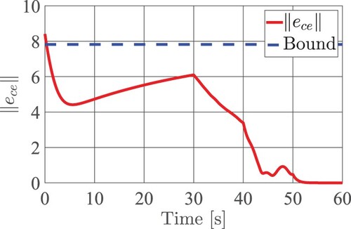
The simulation results are depicted in Figures 6 and 7. Figure 6 shows the time response of the potential function U, and that of the norm of the total control and estimation error $\Vert e_{ce}\Vert$ is depicted in Figure 7. The exponential stability of $\Vert e_{ce}\Vert =0$ is seen from the behaviour after 50s. We also see good tracking performance from the behaviour until 50s, where the potential function U sometimes increases due to the non-zero target object velocity $V_{wo}^b$, but it occurs within the bound as shown in the present analysis. In summary, the present sampled visual feedback pose regulation mechanism works successfully.

Figure 6. Potential function (simulation).

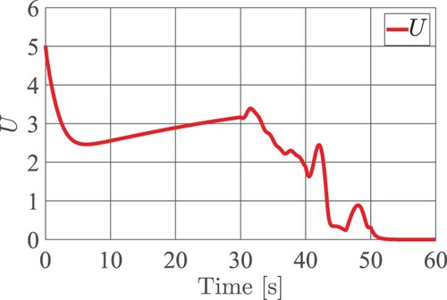
Figure 7. Norm of total error (simulation).

7.2. Experiment

We next show the validity of the present sampled visual feedback pose regulation mechanism (22(22) $\begin{array}{rl}{u}_{ce}\left(t\right)& =K\left[\begin{array}{c}{e}_c\left(t\right)\\ e_e\left(t_i\right)-{\mathrm{A}\mathrm{d}}_{\left(e^{-\hat{\xi }{\theta }_{ce}}\right)}{e}_c\left(t\right)\end{array}\right],t\in [t_i,t_{i+1}),\\ K& :=\left[\begin{array}{cc}{k}_c{I}_6& O_{6\times 6}\\ O_{6\times 6}& k_e{I}_6\end{array}\right]\in {\mathbb{R}}^{12\times 12},k_c,k_e>0.\end{array}$(22) ) via an experiment. Here, two self-developed 2D omnidirectional robots are employed as the camera robot and the target object robot (see Figure 8). In this experiment, the pose estimation is conducted in three-dimensional space, but the pose regulation is demonstrated on two-dimensional plane (x–z plane) with the projection from 6D translational/angular velocity inputs onto 3D ones (i.e. $V_{wc}^b=[v_{wc,x}{v}_{wc,z}{\omega }_{wc,y}{]}^{\mathrm{T}}\in {\mathbb{R}}^3$).

Figure 8. Experimental testbed.

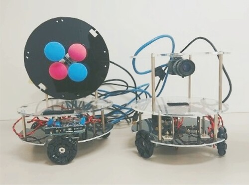
Each omnidirectional robot mainly consists of three motors (RA250100–58Y91 from Daisen Electronics Industrial, Co., Ltd.) with omnidirectional wheels (4571398310089 from Vstone, Co., Ltd.) and a single camera (FL3–U3–13S2C–CS from FLIR Systems, Inc.). The focal length of the camera is tuned as $\sigma =0.0193$ [m], and the camera originally has 120fps. However, when we explicitly consider the image processing time to extract the four feature points attached to the target object robot (see Figure 8), the actual minimum frame rate becomes 18fps in this experiment. We also introduce a motion capture camera system (with OptiTrack Flex13 from NaturalPoint, Inc.) to obtain actual experimental data for the evaluation of the convergence/tracking, but this information is not used for the control inputs of the camera robot.

The present sampled visual feedback pose regulation mechanism (22(22) $\begin{array}{rl}{u}_{ce}\left(t\right)& =K\left[\begin{array}{c}{e}_c\left(t\right)\\ e_e\left(t_i\right)-{\mathrm{A}\mathrm{d}}_{\left(e^{-\hat{\xi }{\theta }_{ce}}\right)}{e}_c\left(t\right)\end{array}\right],t\in [t_i,t_{i+1}),\\ K& :=\left[\begin{array}{cc}{k}_c{I}_6& O_{6\times 6}\\ O_{6\times 6}& k_e{I}_6\end{array}\right]\in {\mathbb{R}}^{12\times 12},k_c,k_e>0.\end{array}$(22) ) with $k_c=2$, $k_e=1.4$, $\delta =0.9$, ${\overline{p}}_{co}=[000.4{]}^{\mathrm{T}}$ [m], and $\overline{\xi }{\overline{\theta }}_{co}=0$ [rad] is applied to the camera robot to achieve the desired relative pose $p_d=[000.33{]}^{\mathrm{T}}$ [m] and $\xi {\theta }_d=0$ [rad]. Here, the initial relative pose is set as $p_{co}\left(0\right)\approx \left[000.37\right]$ [m] and $\xi {\theta }_{co}\left(0\right)\approx 0$ [rad], and the feature points are attached at $p_{o1}\approx [0.020.120.10{]}^{\mathrm{T}}$, $p_{o2}\approx [-0.02-0.080.10{]}^{\mathrm{T}}$, $p_{o3}\approx [0.020.080.14{]}^{\mathrm{T}}$, and $p_{o4}\approx [-0.020.120.14{]}^{\mathrm{T}}$ [m] in ${\mathrm{\Sigma }}_o$. The reference body velocity commands of the target robot are given as follows: $\begin{array}{rl}& \left[\begin{array}{c}{v}_{wo,x}\\ v_{wo,z}\\ {\omega }_{wo,y}\end{array}\right]=\\ & \{\begin{array}{ll}0& t\in [0,10)\\ [\begin{array}{c}-0.025\sin \left({\displaystyle \frac{(t-10)\pi }{10}}\right)\end{array}\\ {\begin{array}{c}0.07\sin \left({\displaystyle \frac{(t-10)\pi }{10}}\right)0\end{array}]}^{\mathrm{T}}& t\in [10,20)\\ {[000.4\sin \left({\displaystyle \frac{(t-20)\pi }{5}}\right)]}^{\mathrm{T}}& t\in [20,25)\\ 0& t\in [25,40)\end{array}.\end{array}$Here, we artificially set the velocity to 0 until 10s and after 25s to verify tracking and convergence in a single demonstration. We also confirmed that the sampling rate of the observer was about 270Hz, which was small enough to be neglected compared with the camera frame rate 18fps.

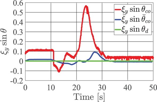
The experimental results are shown in Figures 9–13. Figures 9 and 10 respectively depict the time responses of the potential function U and the norm of the total control and estimation error $\Vert e_{ce}\Vert$. On the other hand, Figures 11–13 show each input/state behaviour focussed on the pose regulation on the 2D experimental field. We see from these figures that the present visual feedback pose regulation mechanism successfully achieves the tracking to the moving target, and the convergence to the desired relative pose to the stationary target is almost achieved. The convergence errors and the tracking delay are due to the physical elements such as the actual dynamics of the robots, the friction between the wheel and the field, and the distortion of the camera image.

Figure 9. Potential function (experiment).

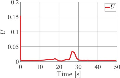
Figure 10. Norm of total error (experiment).

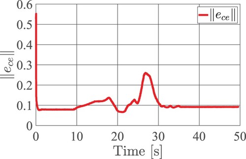
Figure 11. Velocity input command (experiment).

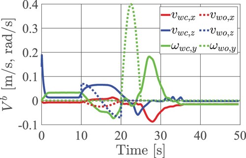
Figure 12. Relative position (experiment).

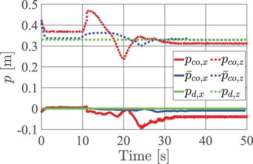
Figure 13. Relative orientation (experiment).

8. Conclusion

This paper presented a vision-based pose observer and its control technique in the sampled data setting by camera frame rates. In the convergence/tracking analysis for the proposed methodologies, we provided the relationship between the frame rates and estimation/control gains. Specifically, we showed that the estimation and control errors are ultimately bounded by a function of the camera frame rate, estimation/control gains, and target object velocity, which provides us with the guidelines for gain settings. The utility of the proposed technique is demonstrated via simulation and an experiment with real hardware.

One of our future directions is to consider robot dynamics. In this regard, previous works [13,16] have already presented passivity-based visual feedback pose regulation mechanisms also for rigid body dynamics in the Euler-Lagrange equation form and the Newton-Euler one. We thus extend the current results with the assistance of these techniques.

Disclosure statement

No potential conflict of interest was reported by the author(s).

Additional information

Funding

This work is supported by the Japan Society for the Promotion of Science (JSPS) KAKENHI [grant number 21K04113].

Notes on contributors

Tatsuya Ibuki

Tatsuya Ibuki received his B.Eng., M.Eng., and Ph.D. degrees in mechanical and control engineering from Tokyo Institute of Technology in 2008, 2010, and 2013, respectively. He was a research fellow with the Japan Society for the Promotion of Science from 2012 to 2013, an assistant professor with the Department of Systems and Control Engineering, Tokyo Institute of Technology from 2013 to 2020, and a visiting scholar with the School of Electrical and Computer Engineering, Georgia Institute of Technology in 2019. Since 2020, he has been a senior assistant professor with the Department of Electronics and Bioinformatics, Meiji University. His research interests include cooperative control of robotic networks, fusion of control theory and machine learning, and vision-based estimation and control.

Satoshi Nakano

Satoshi Nakano received a B.Eng. degree from Nagoya Institute of Technology, Japan, in 2013 and the M.Eng. and Ph.D. degrees in mechanical and control engineering from Tokyo Institute of Technology, Japan, in 2015 and 2019, respectively. Since 2019, he has been an assistant professor in the department of engineering, Nagoya Institute of Technology, Japan. His research interests include nonlinear control, constrained control, and vision-based estimation and control.

Shunsuke Shigaki

Shunsuke Shigaki received his B. Eng., M. Eng., and Ph.D. degrees in mechanical and control system engineering from Tokyo Institute of Technology, Tokyo, Japan in 2013, 2015, and 2018, respectively. He was a JSPS Research Fellowship for Young Scientist (DC1) from 2015 to March 2018, an assistant professor in the division of systems research, Yokohama National University from 2018 to 2019, an assistant professor in the department of system innovation, Osaka University from 2019 to 2023, and a visiting scientist with Max Planck Institute for Chemical Ecology in 2022. He is currently an assistant professor in the principles of informatics research division, National Institute of Informatics, Japan since 2023. His research interests include bio-inspired robotics and algorithms, soft robotics, machine learning, and neuroethology.

Takeshi Hatanaka

Takeshi Hatanaka received a Ph.D. degree in applied mathematics and physics from Kyoto University in 2007. He then held faculty positions at Tokyo Institute of Technology and Osaka University. Since April 2020, he has been an associate professor at Tokyo Institute of Technology. He is the coauthor of “Passivity-Based Control and Estimation in Networked Robotics” (Springer, 2015) and the coeditor of “Economically-enabled Energy Management: Interplay between Control Engineering and Economics” (Springer Nature, 2020). His research interests include cyber-physical-human systems and networked robotics. He received the Kimura Award (2017), Pioneer Award (2014), Outstanding Book Award (2016), Control Division Conference Award (2018), Takeda Prize (2020), and Outstanding Paper Awards (2009, 2015, 2020, 2021, and 2023) all from SICE. He also received 3rd IFAC CPHS Best Research Paper Award (2020) and 10th Asian Control Conference Best Paper Prize Award (2015). He is serving/served as an AE for IEEE TSCT, Advanced Robotics, and SICE JCMSI, and is a member of the Conference Editorial Board of IEEE CSS. He is a senior member of IEEE.

Notes

1 In this equality, we use the homogeneous representation $[p_{ci}^{\mathrm{T}}1{]}^{\mathrm{T}},[p_{oi}^{\mathrm{T}}1{]}^{\mathrm{T}}\in {\mathbb{R}}^4$.

2 Pose estimation/regulation problems with the target object velocity estimation have been tackled in [16].

3 For ease of representation, we often simply use ‘0’ to denote zero vectors with appropriate dimensions.

4 This is easily shown by the properties that $\varphi \left(e^{\hat{\xi }\theta }\right)$ and $\mathrm{s}\mathrm{k}(e^{\hat{\xi }\theta }{)}^{\vee }$ can be respectively rewritten by $1-\cos \theta$ and $\xi \sin \theta$, and thus $\varphi \left(e^{\hat{\xi }\theta }\right)<1$ means $|\theta |<\pi /2$. In this case, $\left(1/2\right)\Vert e_e{\Vert }^2\le U_e\le \Vert e_e{\Vert }^2$ also holds.

References

- Ma Y, Soatto S, Košecká J. An invitation to 3-D vision: from images to geometric models. New York (NY): Springer; 2004.
- Hutchinson S, Hager GD, Corke PI. A tutorial on visual servo control. IEEE Trans Robot Autom. 1996 Oct;12(5):651–670. doi: 10.1109/70.538972
- Chaumette F, Hutchinson S. Visual servo control, part I: basic approaches. IEEE Robot Autom Mag. 2006 Dec;13(4):82–90. doi: 10.1109/MRA.2006.250573
- Chaumette F, Hutchinson S. Visual servo control, part II: advanced approaches. IEEE Robot Autom Mag. 2007 Mar;14(1):109–118. doi: 10.1109/MRA.2007.339609
- AlBeladi A, Ripperger E, Hutchinson S, et al. Hybrid eye-in-hand/eye-to-hand image based visual servoing for soft continuum arms. IEEE Robot Autom Lett. 2022 Oct;7(4):11298–11305. doi: 10.1109/LRA.2022.3194690
- Niu G, Yang Q, Gao Y, et al. Vision-based autonomous landing for unmanned aerial and ground vehicles cooperative systems. IEEE Robot Autom Lett. 2022 Jul;7(3):6234–6241. doi: 10.1109/LRA.2021.3101882
- Zhou S, Miao Z, Zhao H, et al. Vision-based control of an industrial vehicle in unstructured environments. IEEE Trans Control Syst Technol. 2022 Mar;30(2):598–610. doi: 10.1109/TCST.2021.3073003
- Guo D, Jin X, Shao D, et al. Image-based regulation of mobile robots without pose measurements. IEEE Control Syst Lett. 2022 Jan;6:2156–2161. doi: 10.1109/LCSYS.2021.3139288
- Rotithor G, Trombetta D, Kamalapurkar R, et al. Full- and reduced-order observers for image-based depth estimation using concurrent learning. IEEE Trans Control Syst Technol. 2021 Nov;29(6):2647–2653. doi: 10.1109/TCST.2020.3036369
- Bell ZI, Deptula P, Doucette EA, et al. Simultaneous estimation of Euclidean distances to a stationary object's features and the Euclidean trajectory of a monocular camera. IEEE Trans Autom Control. 2021 Sep;66(9):4252–4258. doi: 10.1109/TAC.2020.3035597
- Li Y, Wang H, Xie Y, et al. Adaptive image-space regulation for robotic systems. IEEE Trans Control Syst Technol. 2021 Mar;29(2):850–857. doi: 10.1109/TCST.87
- Keenan P, Janabi-Sharifi F, Assa A. Vision-based robotic traversal of textureless smooth surfaces. IEEE Trans Robot. 2020 Aug;36(4):1287–1306. doi: 10.1109/TRO.8860
- Fujita M, Kawai H, Spong MW. Passivity-based dynamic visual feedback control for three dimensional target tracking: stability and L2-gain performance analysis. IEEE Trans Control Syst Technol. 2007 Jan;15(1):40–52. doi: 10.1109/TCST.2006.883236
- Kawai H, Murao T, Fujita M. Passivity-based visual motion observer with panoramic camera for pose control. J Int Robot Syst. 2011 May;64(3–4):561–583. doi: 10.1007/s10846-011-9557-5
- Ibuki T, Hatanaka T, Fujita M. Visual feedback pose synchronization with a generalized camera model. In: 50th IEEE Conference on Decision and Control and European Control Conference. Orlando, IEEE; 2011. p. 4999–5004.
- Ibuki T, Hatanaka T, Fujita M. Passivity-based visual feedback pose regulation integrating a target motion model in three dimensions. SICE J Control Meas Syst Integr. 2013 Sep;6(5):322–330. doi: 10.9746/jcmsi.6.322
- Yamauchi J, Saito M, Omainska M, et al. Cooperative visual pursuit control with learning of target motion via distributed Gaussian processes under varying visibility. SICE J Control Meas Syst Integr. 2022 Dec;15(2):228–240. doi: 10.1080/18824889.2022.2155454
- Tabuada P. Event-triggered real-time scheduling of stabilizing control tasks. IEEE Trans Autom Control. 2007 Sep;52(9):1680–1685. doi: 10.1109/TAC.2007.904277
- Bemporad A, Heemels M, Johansson M. Networked control systems. London: Springer; 2010.
- Garcia E, Antsaklis PJ. Model-based event-triggered control for systems with quantization and time-varying network delays. IEEE Trans Autom Control. 2013 Feb;58(2):422–434. doi: 10.1109/TAC.2012.2211411
- Ibuki T, Namba Y, Hatanaka T, et al. Passivity-based discrete visual motion observer taking account of camera frame rates. In: 52nd IEEE Conference on Decision and Control. Florence, IEEE; 2013. p. 7660–7665.
- Ibuki T, Walter JR, Hatanaka T, et al. Frame rate-based discrete visual feedback pose regulation: a passivity approach. IFAC Proc Volumes. 2014;47(3):11171–11176. doi: 10.3182/20140824-6-ZA-1003.02768
- Luenberger DG. An introduction to observers. IEEE Trans Autom Control. 1971 Dec;AC–16(6):596–602. doi: 10.1109/TAC.1971.1099826
- Khalil HK. Nonlinear systems. 3rd ed. Upper Saddle River (NJ): Prentice Hall; 2002.