Influences of aerodynamic parameter uncertainties for UFSC based flight trajectory generation

Abstract

This paper discusses the model identification of a biplane which has superior lift generation capability and the influences of identification errors on trajectory generation using updating final-state control (UFSC). Aerodynamic parameters are identified using a combination of wind tunnel tests and computational fluid dynamics (CFD) analysis. The influences of parameter errors on approach trajectory generation are also investigated using Monte Carlo simulations. The simulations clearly demonstrate the relationship between the parameter errors and the trajectory accuracies. In addition, the acceptable range of parameter errors is investigated.

KEYWORDS:

• Fixed-wing UAV
• flight control
• mid-air retrieval
• Monte Carlo simulation
• parameter uncertainty
• UFSC

1. Introduction

Parachutes are widely used in the aerospace field, mainly for mid-air deceleration. For example, a high-altitude balloon for meteorological observation deploys a parachute and descends at a low speed after observations in the sky [1]. The asteroid particles brought back by Hayabusa (JAXA) re-entered the Earth’s atmosphere with a sample capsule and deployed a parachute to mitigate the impact before landing [2]. Furthermore, a parachute shock absorber has been proposed in case the drone breaks down [3].

However, the parachute only reduces the falling speed by increasing the air resistance, and it cannot control the drop point. Therefore, it may cause severe damage if it drops in a residential area or on a busy road. Furthermore, a parachute with a large diameter is required to sufficiently reduce the fall speed, and it may be impossible to achieve a satisfactory deceleration depending on the constraints.

Attempts have been made to conduct mid-air retrievals of objects falling at a planned point using a manned helicopter [4,5]. However, fixed-wing aircraft, which has an excellent cruising range and cruising speed, is preferable over a helicopter to prevent unpredictable accidents. The objective of this study is to achieve mid-air retrieval of a low-speed-descent object using a fixed-wing unmanned aerial vehicle (UAV).

In previous studies by our affiliated research group [6–9], the control law of a fixed-wing UAV was developed for mid-air retrieval of low-speed-descent objects. The control behaviour for approach trajectory generation and impact response control was investigated, and its numerical simulations were conducted. As a partial verification with an experimental aircraft, the trajectory generated by updating final-state control (UFSC) of the feedforward control law generated on the simulation was followed by waypoints. However, flights via UFSC have not yet been achieved because the aircraft used in the experimental system was small, insufficient power was applied for the payload, and the relationship between the microcomputer input and aerodynamic force owing to the control surface was not identified.

In this study, a biplane was adopted as a new airframe that can easily generate sufficient lifts even in the low-speed range to solve these problems and achieve flight by UFSC with an actual aircraft. Next, the aerodynamic parameters required for feedforward control were identified using the fabricated wind tunnel test equipment and computational fluid dynamics (CFD) analysis. In addition, the relationship between UFSC and model predict control (MPC) will be confirmed.

Furthermore, although the identified aerodynamic parameters contain unignorable errors, their influence on the control behaviour has not yet been investigated. In aircraft development, pre-flight evaluations are very important because flight tests in real-world conditions are not easy. As a solution of these issues, Monte Carlo simulations are effective [10]. Probabilistic robustness from Monte Carlo simulations indicates “How likely is the closed-loop system to fail, given limits of parameter uncertainty.” This method can be easily implemented using modern computational and graphical tools [11].

In this paper, we conducted Monte Carlo simulations, assuming that the identified aerodynamic parameters contain errors, and evaluated how the parameter uncertainties would affect approach trajectory generation for low-speed-descent objects. In addition, we adopted a cumulative distribution function to compensate for the lack of computational resources for Monte Carlo simulations. Then, based on the results, we analyzed the permissible error.

The contents in this paper have already been reported in the authors’ position conference paper [12]. This paper presents its journal paper edition including consideration of simulation accuracy from the corresponding symposium paper.

2. Fixed-wing UAV model

2.1. Dynamical system

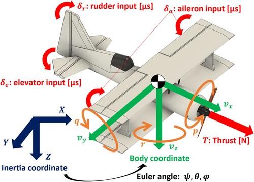
In this section, we define the motion model of the airframe. In a previous study [7], the state equation of a fixed-wing aircraft consisted of a 12-dimensional state vector $\mathit{x}\left(t\right)$ and four-dimensional input vector $\mathit{u}\left(t\right)$. For functions of time $t$, the $\left(t\right)$ notation is henceforth omitted except in special cases. $\mathit{x}$ and $\mathit{u}$ are defined as follows: (1) $\begin{array}{rl}\mathit{x}& ={\left[v_x,v_y,v_z,p,q,r,\psi ,\theta ,\phi ,X,\tilde{Y},\tilde{Z}\right]}^{\text{T}},\\ \mathit{u}& ={\left[{\delta }_a,{\delta }_e,{\delta }_r,T\right]}^{\text{T}},\end{array}$(1) where $v_x,v_y,v_z$ are the velocities in each axial direction of the airframe, $p,q,r$ are the angular velocities around each axis of the airframe, $\psi ,\theta ,\phi$ are the Euler angles, $X$ is the displacement in the forward direction of the airframe in the initial state of the airframe, and $\tilde{Y},\tilde{Z}$ are the reference displacements for approaching the descent object at an arbitrary entry angle. The definition of Euler angle is a rotation matrix that rotates $\psi$ [rad] around the $Z$-axis, then $\theta$ [rad] around the $Y$-axis, and $\phi$ [rad] around the $X$-axis. $\psi ,\theta$ and $\phi$ are called heading angle, pitch angle, and bank angle, respectively [13]. Figure 1 shows a model of the airframe.

Figure 1. Fixed wing UAV model.

It is desirable to be able to approach the aircraft at arbitrary entry angle $\left({\theta }_e,{\psi }_e\right)$ to reflect various conditions. In order to incorporate the parameters $\left({\theta }_e,{\psi }_e\right)$ into the control law, it is necessary to transform the $\left(Y,Z\right)$ coordinates. Figure 2 shows an aircraft approach to a target point at an arbitrary entry angle $\left({\theta }_e,{\psi }_e\right)$. In a previous study [6], the desired trajectory could be generated by introducing the reference displacements $\left(\tilde{Y},\tilde{Z}\right)$. The trajectory indicated by the grey dashed line in Figure 2 is the trajectory without $\left(Y,Z\right)$ coordinate transformation. The dashed grey trajectory is always along the $X$-axis at the terminal time. On the other hand, the black trajectory adopting the reference trajectory $\left(\tilde{Y},\tilde{Z}\right)$ allows entry at the desired entry angle $\left({\theta }_e,{\psi }_e\right)$. The definition of the reference displacement is explained below.

Figure 2. Reference trajectory.

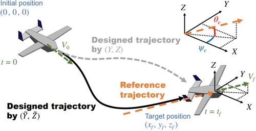
First, a reference trajectory in the direction of the desired reference velocity vector, $V_f$, is determined, as shown in Figure 2. Setting this reference trajectory facilitates the realization of the target approach angle if the aircraft approaches the target point along this trajectory. The reference trajectory has entry angles $\left({\theta }_e,{\psi }_e\right)$ in the horizontal and vertical directions from the $X$-axis, as shown in the upper right part of Figure 2. Equation (2) shows the coordinate transformation from $\left(Y,Z\right)$ to $\left(\tilde{Y},\tilde{Z}\right)$. If the target position coordinates of each axis observed from the current aircraft position are set as $\mathrm{\Delta }X,\mathrm{\Delta }Y,\mathrm{\Delta }Z$, then $\tilde{Y},\tilde{Z}$ can be defined by Equation (2). (2) $\begin{array}{rl}\tilde{Y}& =\mathrm{\Delta }Y\cos {\psi }_e-\mathrm{\Delta }X\sin {\psi }_e\\ \tilde{Z}& =\mathrm{\Delta }Z\cos {\theta }_e-\mathrm{\Delta }X\sin {\theta }_e\end{array}$(2)

2.2. Linear state equation

Although the equation of motion of the aircraft exhibits nonlinear characteristics, the aim of this study is to achieve flight on the control side linearized around the equilibrium point. Therefore, linearization is conducted using the Jacobian matrix around the equilibrium point to analyze it with a linear control law. Linearizing the system expressed using Equation (3) around an arbitrary equilibrium point $\left({\mathit{x}}_{eq},{\mathit{u}}_{eq},{\mathit{y}}_{eq}\right)$ yields a Jacobian matrix as expressed by Equation (4). (3) $\begin{array}{rl}\dot{\mathit{x}}& =f\left(\mathit{x},\mathit{u}\right)\\ \mathit{y}& =h\left(\mathit{x},\mathit{u}\right)\end{array}$(3) (4) $\begin{array}{rl}\mathit{A}& ={\frac{\mathrm{\partial }f\left(\mathit{x},\mathit{u}\right)}{\mathrm{\partial }x}|}_{\left(\mathit{x},\mathit{u}\right)=\left({\mathit{x}}_{eq},{\mathit{u}}_{eq}\right)}\\ \mathit{B}& ={\frac{\mathrm{\partial }f\left(\mathit{x},\mathit{u}\right)}{\mathrm{\partial }u}|}_{\left(\mathit{x},\mathit{u}\right)=\left({\mathit{x}}_{eq},{\mathit{u}}_{eq}\right)}\\ \mathit{C}& ={\frac{\mathrm{\partial }h\left(\mathit{x},\mathit{u}\right)}{\mathrm{\partial }x}|}_{\left(\mathit{x},\mathit{u}\right)=\left({\mathit{x}}_{eq},{\mathit{u}}_{eq}\right)}\\ \mathit{D}& ={\frac{\mathrm{\partial }h\left(\mathit{x},\mathit{u}\right)}{\mathrm{\partial }u}|}_{\left(\mathit{x},\mathit{u}\right)=\left({\mathit{x}}_{eq},{\mathit{u}}_{eq}\right)}\end{array}$(4)

Here in this paper, we assumed that sensing is complete and $\mathit{D}$ is zero matrix. If the difference $\left(\tilde{\mathit{x}},\stackrel{\mathbf{~}}{\mathit{u}},\stackrel{\mathbf{~}}{\mathit{y}}\right)$ between each variable and the equilibrium point is defined by Equation (5), then the system of Equation (3) near the equilibrium point can be linearly approximated as expressed by Equation (6). (5) $\begin{array}{rl}\left(\tilde{\mathit{x}},\stackrel{\mathbf{~}}{\mathit{u}},\stackrel{\mathbf{~}}{\mathit{y}}\right)& =\left(\mathit{x}-{\mathit{x}}_{eq},\mathit{u}-{\mathit{u}}_{eq},\mathit{y}-{\mathit{y}}_{eq}\right)\end{array}$(5) (6) $\begin{array}{rl}\dot{\tilde{\mathit{x}}}& =\mathit{A}\stackrel{\mathbf{~}}{\mathit{x}}+\mathit{B}\stackrel{\mathbf{~}}{\mathit{u}}\\ \tilde{\mathit{y}}& =\mathit{C}\stackrel{\mathbf{~}}{\mathit{x}}\end{array}$(6)

An equilibrium point exists for the airframe, depending on the air speed. The equilibrium point was determined in the wind tunnel test described in the next section.

2.3. Aerodynamic parameter identification

This paper deals with fixed-wing UAVs. The motion of a fixed-wing aircraft is described by an aerodynamic force that is proportional to the dynamic pressure. One of the parameter of aerodynamic force is the aerodynamic dimensionless coefficient [14,15]. The aerodynamic dimensionless coefficients are linear parameters that represent the rate of change of forces and moments with respect to changes in the attitude and input of the aircraft. Each parameter has the following meaning: (7) $C_{A_B}=\frac{\mathrm{\partial }{C}_A}{\mathrm{\partial }B},$(7) where B is a parameter that varies and A is an axis of force or moment that varies in proportion to B.

In a previous study [8], an experimental system was constructed using the monoplane Savanna (Atorie_m_m), and aerodynamic dimensionless coefficients were identified through CFD analysis. However, Savanna is a small and light aircraft, and it was unsuitable for collecting objects or carrying a large payload. Therefore, the airframe used for the experimental system in this study was changed to MAMBA10 (Flex Innovation) [16], and the experimental system was reconstructed.

In this study, we aimed to develop an approach to descent objects through feedforward control. Feedforward control requires a known airframe model, and the aerodynamic performance of an actual aircraft varies significantly depending on the effects of the propeller slipstream and the surface shape of the airframe. In order to improve the accuracy of the model under control as much as possible, the identification was based on the results of wind tunnel tests whenever possible. However, it was difficult to identify $C_{m_q},C_{l_p},C_{l_r},C_{n_p},C_{n_r}$ which are related to the change in angular velocity. Therefore, we adopted CFD as an alternative method to identify $C_{m_q},C_{l_p},C_{l_r},C_{n_p},C_{n_r}$, referring to a previous report [8].

We manufactured a wind tunnel test device before conducting the wind tunnel tests. The manufactured test device could freely change the angle of attack using a servomotor. The forces and moments generated in the airframe were measured by connecting the device to the upper part of the load cell. Wind tunnel tests were conducted using this test device and blowout wind tunnel. Figure 3 shows a photograph of the overall view during the wind tunnel tests.

Figure 3. Photograph of wind tunnel test setup.

The wind tunnel tests were conducted at a blow velocity of 15 m/s, and the equilibrium point at that time was identified while varying the thrust and the angle of attack. We obtained the aerodynamic dimensionless coefficients by changing the state of the airframe around the identified equilibrium point. However, it was difficult to apply the wind tunnel test to obtain the aerodynamic dimensionless coefficients of the aerodynamic force caused by the change in angular velocity; hence, we used XFLR5 to perform the CFD analysis [17].

XFLR5 was used to identify the aerodynamic dimensionless coefficients in Savanna [8]. This tool was adopted because analysis in the low-Reynolds region was expected, and a biplane model existed. XFLR5 has design and analysis functions for 3D wing models based on the lifting-line theory, vortex lattice method, and 3D panel method. The equilibrium point and aerodynamic dimensionless coefficients can be analyzed by blowing a uniform flow at regular intervals on a model established on XFLR5. Figure 4 shows the model used for the analysis with XFLR5. The airfoil shapes of the main wing, vertical stabilizer, and horizontal stabilizer were estimated from their geometrical shapes; they are denoted NACA23012, NACA0008, and NACA0012, respectively. Table 1 lists each identified parameter of MAMBA 10. We used the values obtained via CFD analysis with XFLR5 for $C_{m_q},C_{l_p},C_{l_r},C_{n_p},C_{n_r}$, which are aerodynamic dimensionless coefficients in Table 1. Furthermore, $C_{m_u}$ was assumed to be zero because the cruising speed was low.

Figure 4. Model used for CFD analysis.

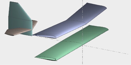
Table 1. Airframe parameters of MAMBA 10.

Parameter	Value	Parameter	Value
$C_{L_0}$[-]	0.158	$M$[kg]	2.00
$C_{D_0}$[-]	0.111	$S$[m^2]	0.446
$C_{L_{\alpha }}$[1/rad]	1.59	$b$[m]	1.03
$C_{D_{\alpha }}$[1/rad]	1.31	$\overline{c}$ [m]	0.216
$C_{m_0}$[-]	0.0595	$I_x$[kg-m^2]	0.0470
$C_{m_u}$[-]	0.0	$I_y$[kg-m^2]	0.0862
$C_{m_{\alpha }}$[1/rad]	−1.85	$I_z$[kg-m^2]	0.107
$C_{m_q}$[-]	−6.13	$v_{x_{eq}}$[m/s]	14.4
$C_{m_{{\delta }_e}}$[1/$\mu \text{s}$]	−0.00061	$v_{z_{eq}}$[m/s]	1.51
$C_{l_{\text{β}}}$[1/rad]	−0.0963	${\theta }_{eq}$[rad]	0.105
$C_{l_p}$[-]	−0.323	${\delta }_{a_{eq}}$[$\mu \text{s}$]	1500
$C_{l_r}$[-]	0.0925	${\delta }_{a_{min}}$[$\mu \text{s}$]	1000
$C_{l_{{\delta }_a}}$[1/$\mu \text{s}$]	0.000418	${\delta }_{a_{max}}$[$\mu \text{s}$]	2000
$C_{l_{{\delta }_r}}$[1/$\mu \text{s}$]	−0.00016	${\delta }_{e_{eq}}$[$\mu \text{s}$]	1280
$C_{n_{\text{β}}}$[1/rad]	0.0676	${\delta }_{e_{min}}$[$\mu \text{s}$]	1000
$C_{n_p}$[-]	−0.147	${\delta }_{e_{max}}$[$\mu \text{s}$]	2000
$C_{n_r}$[-]	−0.230	${\delta }_{r_{eq}}$[$\mu \text{s}$]	1500
$C_{n_{{\delta }_a}}$[1/$\mu \text{s}$]	−0.000074	${\delta }_{r_{min}}$[$\mu \text{s}$]	1000
$C_{n_{{\delta }_r}}$[1/$\mu \text{s}$]	−0.00014	${\delta }_{r_{max}}$[$\mu \text{s}$]	2000
$C_{y_{\text{β}}}$[1/rad]	−0.373	$T_{eq}$[N]	14.0
$C_{y_{{\delta }_r}}$[1/$\mu \text{s}$]	0.000174	$T_V$[N/V]	1.78
		$T_{min}$[N]	0.0
		$T_{max}$[N]	20.0 (at 21.5 V)

For inputs ${\delta }_a,{\delta }_e,{\delta }_r$, the input signal to the servomotor that derives the control surface was adopted instead of the angle of the aileron, elevator and rudder. The servo motor uses the pulse width of the PWM signal as the input signal [18]. This eliminates the need to identify the relationship between the arm of the servomotor and the change in the steering angle. Although ESC (Electric Speed Controller) that powers the brushless motor also uses the pulse width of the PWM signal, thrust $T$ is expressed in [N]. This is because the relationship between the battery voltage $V$ and the PWM signal sent to the ESC was identified by wind tunnel test.

3. Control method

Retrieval of a descent object requires the precise arrival of the airframe at a specified place and time. To achieve this condition, we adopted UFSC as an optimal control problem of the fixed terminal state and fixed terminal time for approach trajectory design in this study. This control law compensates for errors caused by linearization and disturbances by recalculating the final-state control (FSC), an optimal control problem with a fixed terminal state and fixed terminal time, at every arbitrary control step.

First, because FSC deals with linear discrete time, Equation (6) must be transformed into a controllable n-dimensional m-input linear discrete-time system as expressed by Equation (8): (8) $\begin{array}{rl}\mathit{x}\left[k+1\right]& ={\mathit{A}}_d\mathit{x}\left[k\right]+{\mathit{B}}_d\mathit{u}\left[k\right],\\ \mathit{y}\left[k\right]& ={\mathit{C}}_d\mathit{x}\left[k\right],\end{array}$(8) where $k$ is the number of control steps. Let $N$ be the number of control steps up to the target, and assume transition from the initial state $\mathit{x}\left[0\right]$ to the final state $\mathit{x}\left[N\right]$.

Next, the feedforward input matrix $\mathit{U}$ and evaluation function $J$ are defined as follows: (9) $\begin{array}{rl}\mathit{U}& =\left[{\mathit{u}}^{\text{T}}\left[N-1\right]\dots {\mathit{u}}^{\text{T}}\left[1\right]{\mathit{u}}^{\text{T}}\left[0\right]\right],\end{array}$(9) (10) $\begin{array}{rl}J& ={\mathit{U}}^{\text{T}}\stackrel{\mathbf{~}}{\mathit{R}}\mathit{U},\end{array}$(10) where $\tilde{\mathit{R}}$ is an $mN\times mN$ positive definite-weight matrix. The feedforward input matrix, $\mathit{U}$, that minimizes the evaluation function, $J$, in Equation (10) is the control input group via FSC. If $\mathit{\Sigma }$ is defined as given by Equation (11), then $\mathit{U}$ is uniquely determined using Equation (12). (11) $\begin{array}{rl}\mathit{\Sigma }& =\left[{\mathit{B}}_d{\mathit{A}}_d{\mathit{B}}_d\dots {{\mathit{A}}_d}^{N-2}{\mathit{B}}_d{{\mathit{A}}_d}^{N-1}{\mathit{B}}_d\right]\end{array}$(11) (12) $\begin{array}{rl}\mathit{U}& ={\tilde{\mathit{R}}}^{-1}{\mathit{\Sigma }}^{\text{T}}(\mathit{\Sigma }{\tilde{\mathit{R}}}^{-1}{\mathit{\Sigma }}^{\text{T}}{)}^{-1}\left\{\mathit{x}\left[N\right]-{\mathit{A}}_d^N\mathit{x}\left[0\right]\right\}\end{array}$(12)

The ${\tilde{\mathit{R}}}^{-1}{\mathit{\Sigma }}^{\text{T}}(\mathit{\Sigma }{\tilde{\mathit{R}}}^{-1}{\mathit{\Sigma }}^{\text{T}}{)}^{-1}$ part, which is the left portion on the right-hand side of Equation (12), is uniquely obtained regardless of the airframe state. Therefore, only the $\left\{\mathit{x}\left[N\right]-{\mathit{A}}_d^N\mathit{x}\left[0\right]\right\}$ part, which is the right portion on the right-hand side, is calculated during the flight of an actual aircraft.

However, the actual motion is nonlinear, and errors attributed to linear approximation always occur. In addition, disturbances such as wind may change the airframe coordinates and the target position, and equivalent disturbances might occur owing to errors in the identified airframe parameters. Therefore, UFSC, which updates the terminal state $\mathit{x}\left[N\right]$ for every arbitrary control step and recalculates the feedforward input matrix, $\mathit{U}$, was adopted instead of FSC for the approach trajectory generation to solve these problems.

Here, we also consider the relationship between MPC and UFSC. MPC is a commonly used approach trajectory generation method, and it has been shown that MPC and UFSC have the same control law under certain conditions by the authors’ group in [6]. However, the problem in this paper does not satisfy the conditions. This paper especially focuses on the final state of the aircraft and deal with a positioning control problem. UFSC is considered to be advantageous in such a problem setting because it is less computationally than standard MPC. On the other hand, MPC can also be taken account of some constrained conditions such as the maximum control input. However, the addition of constraint conditions dramatically increases the computation load and makes it difficult to implement on actual equipment [6]. Therefore, this paper focuses on the application of UFSC.

4. Simulation

4.1. Simulation method

In the previous section, UFSC was adopted to eliminate the effects of errors. However, the evaluation of the influence of the error of the airframe parameters has not yet been conducted. The study conducted by our research group to date has been based on the assumption that all parameters are obtained under ideal conditions. However, the airframe parameters analyzed in this study are expected to contain errors. In particular, aerodynamic dimensionless coefficients include measurement errors and variations attributed to the mounting of sensors on the airframe surface and scratches.

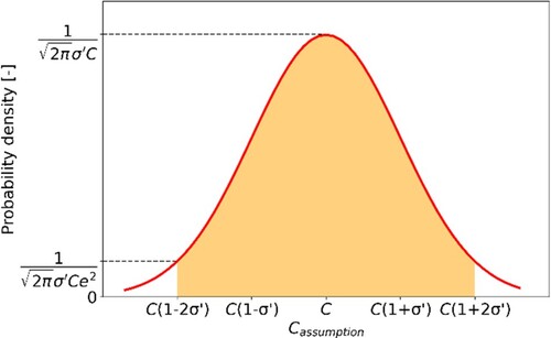
Therefore, it is necessary to investigate the influence of parameter uncertainty in advance and determine the acceptable error. In this study, we focused on the aerodynamic dimensionless coefficients, assumed to have a relatively significant identification error. We assumed that the value obtained by adding the error to the identified aerodynamic dimensionless coefficients is the true value $C_{assumption}$, and we conducted numerical simulations to evaluate the effect of the error. $C_{assumption}$ is defined for every parameter listed on the right-hand side of Table 1.

First, $C_{assumption}$ was defined. $C_{assumption}$ should not deviate significantly from the identified parameters. Furthermore, all parameter errors should not be manipulated arbitrarily. Therefore, we assumed that $C_{assumption}$ exists according to the existence probability of normal distribution for dimensionless aerodynamic parameters with reference to the literature [19]. Moreover, the average $E\left(C_{assumption}\right)$ and the standard deviation $\sigma$ of each $C_{assumption}$ was determined using Equation (13): (13) $\begin{array}{rl}& E\left(C_{assumption}\right)=C,\\ & \sigma ={\sigma }^{\mathrm{\prime }}C,\end{array}$(13) where ${\sigma }^{\mathrm{\prime }}$ is a coefficient, and $C$ is an arbitrary aerodynamic dimensionless coefficient. $C_{assumption}$ was assumed to exist within the range shown in Figure 5 to prevent a sudden occurrence of a significantly large error. Therefore, the range of $C_{assumption}$ is expressed by Equation (14). (14) $C\left(1-2{\sigma }^{\mathrm{\prime }}\right)\le C_{assumption}\le C\left(1+2{\sigma }^{\mathrm{\prime }}\right)$(14)

Figure 5. Range over which true values exist.

Simulations were conducted by numerical integration using the fourth-order Runge–Kutta method. The values listed in Table 1 were used to calculate the control input, and the values on the left-hand side of Table 1 and $C_{truth}$ were used to calculate the motion of the airframe.

UFSC tends to diverge when the number of remaining steps is small. Based on the authors’ previous report [20], the UFSC method applied in this paper stops updating the control input by recalculation when horizon is less than 10 steps. This suppressed the divergence of the control inputs without increasing the computation time.

The Monte Carlo method was used to perform error evaluation. The Monte Carlo method was adopted because it has the following advantages [21].

1. Direct evaluation of nonlinear systems is possible.

2. The effects of multiple uncertain parameters are visible in the results.

3. Computation load is independent of the number of uncertain parameters because it is a sample study.

Table 2 lists the simulation conditions. We redefined $C_{assumption}$ for each trial and conducted numerical simulations. We carried out 100 trials for each of the four conditions (${\sigma }^{\mathrm{\prime }}=0.05,0.1,0,2,0.3$), and the statistics of the deviation from the target coordinates at the target time were obtained. The number of trials for each condition was set to 100, due to the computational resources of the research group's PCs. This number of trials was chosen as a condition that can be computed in a few days in the authors’ computing environment. Then, the expected value of the error and retrievable probability were determined, and the magnitude of the allowable error was investigated.

Table 2. Simulation conditions.

Simulation conditions	Value
${\sigma }^{\mathrm{\prime }}$	0.05, 0.1, 0.2, 0.3
Weight matrix	$\text{Diag}\left(1,{10}^5,1,{10}^3\right)$ $\otimes {\mathit{I}}_{100}$
Initial coordinate [m]	(0, 0, 0)
Initial state	Equilibrium point
Target coordinate [m]	(140, 30, −5)
Entering angle [rad]	(0, 0)
Approach time [s]	10
Discrete time in 1 step [s]	0.1
UFSC updating time [s]	0.5
Number of trials	100 × 4

4.2. Simulation results

Figure 6 shows the simulation results. The upper two graphs in Figure 6 show the trajectories on the $X$-$Y$ and $X$-$Z$ planes, and the lower four graphs show the time variations in the aileron input, elevator input, rudder input, and thrust. The black line in Figure 6 indicates the trajectory and input when no parameter error occurs, and the purple line indicates the input value at the target coordinates and equilibrium point. For comparison, Figure 7 shows the results of a simulation controlled by FSC under the conditions in Table 2.

Figure 6. UFSC simulation results.

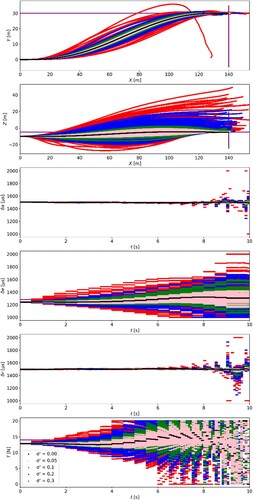
Figure 7. FSC simulation results.

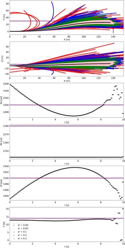
The trajectory and control inputs diverge from the ideal conditions as the parameter error increases (Figure 6). Comparing the inputs in Figures 6 and 7, the control inputs for FSC is the same under all conditions. On the other hand, UFSC shows that the larger the parameter errors, the larger the value of the inputs changes. Furthermore, unlike FSC, UFSC trajectory tends to converge to the target coordinates as the target time approaches. Hence, the UFSC works as a pseudo-feedback for parameter errors.

Figure 8 shows the histogram of the errors in the straight-line distance from the target coordinates at the target time for each condition. Note that cases where the error in the straight-line distance is 5 m or more are collectively displayed. The accuracy of the approach trajectory generation decreases as the parameter error increases (Figure 8). Similarly, Table 3 shows the correlation between parameters and approach trajectory errors.

Figure 8. Histogram of errors.

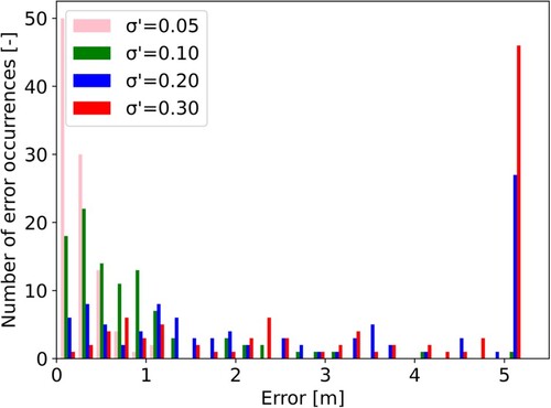
Table 3. Result of the Monte Carlo simulation.

$\sigma {}^{\mathrm{\prime }}$	Probability of error within 1 metre [%]
0.05	98
0.1	77
0.2	25
0.3	15

In order to eliminate the effect of errors due to width of the bins, we adopted the cumulative distribution function for approximation. The approach trajectory errors are assumed to be exponentially distributed, and we consider an approximation with the exponential distribution. First, the exponential distribution $f\left(x\right)$ is generally represented by Equation (15): (15) $f\left(x\right)=\lambda e^{-\lambda x}\left(x\ge 0\right),$(15) where $\lambda$ is a positive constant. The expected value, $E$, and variance, $V$, of the exponential distribution are expressed by Equation (16). (16) $\begin{array}{rl}E& =\frac{1}{\lambda }\\ V& =\frac{1}{{\lambda }^2}\end{array}$(16)

The cumulative distribution function $F\left(x\right)$ is used to obtain a more accurate approximation. The cumulative distribution function is the integral of $f\left(x\right)$, and the cumulative distribution function of the exponential distribution is expressed as follows. (17) $F\left(x\right)=1-e^{-\lambda x}\left(x\ge 0\right)$(17) The cumulative distribution obtained by the simulation is approximated to Equation (17) using the least-squares method. We discuss the possibility of retrieval from the parameters obtained using this equation. Figure 9 shows the cumulative distribution and approximation curve of the simulation results.

Figure 9. Cumulative distribution of errors.

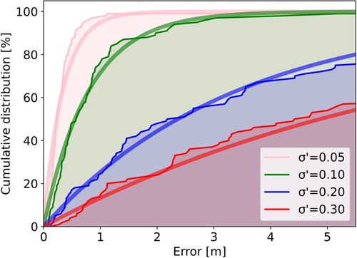
Each approximation curve can approximate the exponential distribution with high accuracy (Figure 9). Moreover, the error range is within approximately 1 m when ${\sigma }^{\mathrm{\prime }}=0.05$ and approximately 3 m when ${\sigma }^{\mathrm{\prime }}=0.10$. In contrast, in the case of ${\sigma }^{\mathrm{\prime }}=0.20,0.30$, there is a possibility of a relatively large error generation. Table 4 presents the relationship between parameter error and approach trajectory accuracy using an approximated graph.

Table 4. Influences of parameter error on approach trajectory.

$\sigma {}^{\mathrm{\prime }}$	$\lambda$[1/m]	$E$[m]	$V$[m^2]	Probability of error within 1 metre [%]
0.05	2.96	0.337	0.114	94.8
0.1	1.26	0.795	0.632	71.6
0.2	0.293	3.41	11.6	25.4
0.3	0.142	7.03	49.4	13.3

In the simulations, retrieval was considered successful when the error with the target coordinates at the target time was within 1 m or less. Based on the parameters identified in this study, retrieval was possible with a high probability if ${\sigma }^{\mathrm{\prime }}=0.05$. Therefore, the error of the aerodynamic dimensionless coefficients should be controlled within $\pm 10\mathrm{\%}$. With an increase to ${\sigma }^{\mathrm{\prime }}=0.10$, the retrieval success probability decreases to approximately 70%. For realistic retrieval, the identification error of aerodynamic dimensionless coefficients must be limited to approximately $\pm 20\mathrm{\%}$.

5. Conclusion

In this study, we investigated the model identification of the experimental aircraft and the influence of the model error on approach trajectory generation. In a previous study [7], partial verification was conducted using an experimental aircraft. However, it was challenging to achieve mid-air retrieval of a low-speed-descent object owing to aspects such as the mounting capacity of the airframe. Therefore, we adopted a biplane that easily generated lift and used it as an experimental aircraft. Furthermore, the aerodynamic dimensionless coefficients were identified using wind tunnel tests and CFD analysis because the airframe parameters must be known for a UFSC flight.

Because these aerodynamic dimensionless coefficients were expected to contain identification errors, we investigated the impact of parameter errors on approach trajectory generation. Monte Carlo simulation was used as the investigation method, and the retrieval accuracy and success probability were obtained for each size of the identification error. In addition, the role of pseudo-feedback from UFSC recalculations was confirmed. Furthermore, the allowable error range of the parameters was determined based on the simulation results. Moreover, feedforward control of unmodelled factors such as disturbances is discussed.

One of the future issues is the need to make the more accurate model for CFD analysis. The model of the aircraft used in the CFD analysis did not include the propeller, and did not consider the effect of the propeller and its slipstream. This point needs to be resolved, and the numerical consistency between the two identification methods needs to be investigated by fully matching the conditions with the wind tunnel test.

The Monte Carlo simulation method also has future issues. First, aerodynamic parameters interactions such as the relationship between $C_L$ and $C_D$ need to be considered in the simulations. In this study, each aerodynamic dimensionless coefficients error was independent each other, but consideration should be given to including correlations in the aerodynamic parameters. In addition, the number of trials was not sufficient due to limited computer resources. Therefore, after a sufficient computing environment is established, the level of significance should be defined and the simulation should be performed to satisfy the level of significance.

Future investigations include conducting a flight test of the airframe with the identified parameters and investigating the reliability of the identified parameters from the logs of the state quantities of the airframe in the trim state. Additionally, we will investigate whether the parameter identification is enough accurate for flight control by UFSC. If aerodynamic dimensionless coefficients can be identified with sufficient accuracy, then experimental autonomous flight tests will be conducted using UFSC.

Disclosure statement

No potential conflict of interest was reported by the author(s).

Additional information

Funding

This work was supported by The Takahashi Industrial and Economic Research Foundation: [Grant Number 12-001-39].

Notes on contributors

Fumiaki Hirahara

Fumiaki Hirahara He received the B.S. and M.S degrees in engineering from Nagoya University, Nagoya, Japan, in 2021 and 2023 respectively.

Kandai Uchida

Kandai Uchida He received the B.S. degrees in engineering from Nagoya University, Nagoya, Japan, in 2022 respectively.

Susumu Hara

Susumu Hara He received the B.S., M.S., and Ph.D. degrees in engineering from Keio University, Tokyo, Japan, in 1992, 1994, and 1996, respectively. In 2008, he joined the Faculty of Nagoya University, Nagoya, where he is currently a Professor with the Department of Aerospace Engineering, Graduate School of Engineering. His current research interests include motion and vibration control of mechanical structures, nonstationary control methods, control problems of man-machine systems, and aerospace equipment.

References

- High-level weather observation by radiosonde [Internet]. Japan: Meteorological Agency; [cited 2023 Mar 31]. Available from: https://www.jma.go.jp/jma/kishou/know/upper/kaisetsu.html.
- Bringing HAYABUSA Back to Earth [Internet]. Japan: JAXA; [cited 2023 Mar 31]. Available from: https://global.jaxa.jp/article/special/hayabusareturn/kawaguchi01_e.html.
- Ichihara K. Technologies and applications in the drone industry. J Japan Inst Electron Pack. 2016;19(6):408–415.
- Lo ML, Williams BG, Bollman WE, et al. Genesis mission design. J Astronaut. 2001;49(1):169–184.
- Darley M, Beck P. Return To sender: lessons learned from rocket lab’s first recovery mission. Proceedings of the Small Satellite Conference; 2021 Aug 7–12; Logan, Utah (UT):2021.
- Hara S, Yokoo R, Miyata K. Understanding the final-state control from the standpoint of the model predictive control and its application to a three-dimensional trajectory control problem. Microsyst. Technolo. 2020;26(1):49–57. doi:10.1007/s00542-019-04397-0
- Nakamura S, Takeuchi S, Hara S, et al. Toward the realization of mid-air retrieval of low-speed-descent objects by means of fixed-wing UAVs). Proceedings of the JSME 2020 Conference on Robotics and Mechatronics; 2020 May 27–30; Kanazawa, Japan.
- Takeuchi S, Nakamura S, Hara S, et al. Updating final-state control methods taking input constraints at final time into account (adaptive flight trajectory design of fixed-wing UAVs). J Adv Mech Des Syst Manuf. 2020;14(7):JAMDSM0106–JAMDSM0106. doi:10.1299/jamdsm.2020jamdsm0106
- Hirai M, Hirahara F, Hara S, et al. Mid-Air retrieval control for low-speed-decent objects by switching from updating final state control to adaptive nonstationary control. Proceedings of the 59th Aircraft Symposium; 2021 Nov 30–Dec 2; Tokushima, Japan.
- Motoda T. Stochastic system evaluation by Monte Carlo simulation. Japan: JAXA; 2007; (JAXA Research and Development Report; JAXA-RR-07-005).
- Stengel RF, Ryan LE. Stochastic robustness of linear time-invariant control systems. IEEE Trans. Automat. 1991;36(1):82–87. doi:10.1109/9.62270
- Hirahara F, Uchida K, Hara S. Influences of parameter uncertainties for UFSC based flight trajectory generation of a biplane model. Proceedings of the SICE International Symposium on Control Systems 2023; 2023 Mar 9–11; Shiga, Japan.
- Duke EL, Antoniewicz RF, Krambeer KD. Derivation and definition of a linear aircraft model. USA: NASA; 1988; (NASA Reference Publication 1207).
- Lykins R, Riley R, Garcia G, et al. Modal analysis of 1/3-scale yak-54 aircraft through simulation and flight testing. AIAA Atmospheric Flight Mechanics Conference; 2011 Aug 8–11; Portland, Oregon (OR):2011.
- Jung D, Tsiotras P. Modeling and hardware-in-the-loop simulation for a small unmanned aerial vehicle. AIAA Infotech @ Aerospace Conference and Exhibit; 2007 May 7–10; Rohnert Park, California (CA):2007.
- MAMBA 10 G2 SUPER PNP [Internet]. Florida (FL): Flex Innovations; [cited 2023 Mar 31]. Available from: https://www.flexinnovations.com/product/mamba-10-g2-super-pnp/.
- xflr5 [Internet]. place unknown: publisher unknown; [cited 2023 Mar 31]. Available from: http://www.xflr5.tech/xflr5.htm.
- Hadi GS, Varianto R, Trilaksono BR, et al. Autonomous UAV system development for payload dropping mission. J Instrum Autom Syst. 2014;1(2):72–77. doi:10.21535/jias.v1i2.158
- Stengel RF. Some effects of parameter variations on the lateral-directional stability of aircraft. J Guid. Control Dyn. 1980;3(2):124–131. doi:10.2514/3.55959
- Hirahara F, Hirai M, Hara S, et al. Investigation and simulation of an actual system for aerial retrievals of low-speed falling objects. Proceedings of the JSME 2022 Conference on Robotics and Mechatronics; 2022 Jun 1–4; Sapporo, Japan.
- Motoda T. Detection of influential uncertain parameters in Monte Carlo evaluation. J Jpn Soc Aeronaut Space Sci. 2007;55(638):117–124.