
 ?Mathematical formulae have been encoded as MathML and are displayed in this HTML version using MathJax in order to improve their display. Uncheck the box to turn MathJax off. This feature requires Javascript. Click on a formula to zoom.
ABSTRACT
This paper discusses ‘strong-form’ frequentist testing as a useful complement to null hypothesis testing in communication science. In a ‘strong-form’ set-up a researcher defines a hypothetical effect size of (minimal) theoretical interest and assesses to what extent her findings falsify or corroborate that particular hypothesis. We argue that the idea of ‘strong-form’ testing aligns closely with the ideals of the movements for scientific reform, discuss its technical application within the context of the General Linear Model, and show how the relevant P-value-like quantities can be calculated and interpreted. We also provide examples and a simulation to illustrate how a strong-form set-up requires more nuanced reflections about research findings. In addition, we discuss some pitfalls that might still hold back strong-form tests from widespread adoption.
Concerns about the validity of research findings have been at the forefront of scientific debate over the past decade. This is also true in communication science, where movements for reform have recently been gaining more and more traction (Dienlin et al., Citation2020). Philosophically speaking, many arguments of such movements are falsificationist in spirit (Lakatos, Citation1978; Mayo, Citation2018; Popper, Citation1963; see also, Derksen, Citation2019): they stress that scientific claims should be considered viable only to the extent that they passed heavy scrutiny and stringent testing. To this end, policy surrounding the transparency of research methods, pre-registration of research hypotheses, and replication of results are being advocated and implemented. However, there is yet another way in which communication science, much like other behavioral sciences, could gear itself toward falsificationist ideals: by rethinking statistical practice. Traditionally, communication scientists have relied disproportionally on a statistical routine known as null hypothesis significance testing, also referred to as NHST (Levine, Weber, Hullet, Park, & Lindsey, Citation2008; Vermeulen et al., Citation2015). In NHST, a substantive research hypothesis (e.g., 'violent video game play influences aggressive cognitions') is evaluated on the basis of a -value associated with a test of the statistical nil-null hypothesis ('there is no relationship between video game play and aggressive cognitions'). Whenever the
-value lies below a conventional threshold denoted by α – usually,
– the finding is said to be statistically significant, which is taken to mean that there is an ‘effect’ or ‘difference’ (e.g., 'violent video game play significantly influences aggression'). In all other cases, the result is considered not statistically significant, which is interpreted as absence of evidence for, or evidence against, an effect or difference (e.g., “violent video game play did not significantly influence aggression”).
There are two well-known issues with this approach – both of which hamper its value as a means for stringent hypothesis testing. First, NHST leaves much of the actual statistical logic to conventional decision rules and the behavior of software. Researchers choose a statistical model for the data at hand and report the results as expected by APA-standards, but they rarely confront the inferential meaning of their results. They stick to a binary conclusion of a finding being ‘significant’ or not, which ignores more fundamental reflections about the strength of a finding or its theoretical relevance. As a consequence, the evidence gleaned from NHST – in particular, the -value – is known to be often misrepresented and overblown (e.g., Greenland, Senn, Rothman, Carlin, Poole, Goodman, & Altman, Citation2016; Nickerson, Citation2000; Vermeulen et al., Citation2015). A second, and even more fundamental, problem with NHST is that it is generally unable to say anything useful about hypotheses of substantive interest. This is true even when the
-values derived from the test are, technically speaking, correctly interpreted: the nil hypothesis is set up as a straw man (i.e., the claim that not the tiniest effect or relation exists between the variables of interest), and its rejection (or lack thereof) tells us little about the types of substantive hypotheses researchers are typically interested in (e.g., De Groot, Citation1956/2014; Meehl, Citation1967, Citation1990). Indeed, when pressed, communication researchers would probably not claim to be interested in infinitesimally small effects. Much of communication science is conducted within an aura of social relevance. Time and money is spent on investigating the impact of communication styles and technology because it is believed that there might, in fact, be substantial and replicable effects that require regulation and/or intervention.
-values derived from NHST seem of little help in such a scenario.
In light of these issues, many voices have been calling for statistical reforms that move away from NHST, the use of -values, and even frequentist statistics in general (for an overview, see the special issue in the American Statistician: Wasserstein et al., Citation2019). In this paper, we will not take such a fundamental stance. Rather, we will try to familiarize communication scientists with one line of thought within the reform movement that remains close to the familiar
-value concept but aligns it with the falsificationist ideal of stringent hypothesis testing. After Meehl (Citation1967), Meehl (Citation1990), we label this approach ‘strong-form’frequentist testing' – although its core principles reside under different names as well (e.g., ‘severe testing’: Mayo, Citation2018; Mayo & Spanos, Citation2006; ‘minimal effect testing’: Murphy & Myors, Citation1999; ‘(non-)equivalency testing’: Weber & Popova, Citation2012; Wellek, Citation2010). The basic idea of strong-form testing is straightforward: instead of testing a nil-null-hypothesis we simply set up a test for a statistical hypothesis of (minimal) theoretical interest. This provides us with a different kind of
-value – which, in this paper, we choose to denote by
– that may be more directly interpreted as a measure of falsifying or corroborating evidence (see also, Greenland, Citation2019; Haig, Citation2020): it provides information on how much evidence the data offer to refute (or corroborate) the hypothesized effect size of (minimal) interest.
In what follows, we first provide a refresher of key concepts within the frequentist hypothesis testing framework – in particular, sampling distributions, test statistics, -values, and statistical power. Readers who are knowledgeable of frequentist inference will find the information in this section familiar and may decide to skip it entirely; the value in this part mainly lies in (1) gradually introducing the logic and terminology of frequentist statistics (which seems useful for non-expert audiences), (2) clarifying some terminological choices made in the paper, and (3) showing that the ‘strong-form’ construal flows naturally from a properly conceptualized frequentist logic. In the second part of the paper we formulate general guidelines for the application of strong-form testing within the context of the General Linear Model: we show how
can be calculated, discuss some important considerations when interpreting
, and we illustrate its behavior through a simulation. In the last part of the paper, we consider some technical challenges for strong-form testing in more complicated use-cases, and we suggest pathways for future developments.
The meaning of P
While the -value lies at the heart of statistical inference in communication science, the concept is notoriously misunderstood (Vermeulen et al., Citation2015). Some widespread misconceptions are, for instance, that
-values represent the probability that the null hypothesis is true, that they reflect the probability of results being replicable, or that small
-values imply practically important effects (e.g., Greenland et al., Citation2016; Nickerson, Citation2000). If we want to understand what
-values represent, we first need to be familiar with two key concepts from frequentist statistics: sampling distributions and test statistics. Sampling distributions form the building blocks of frequentism; they represent the theoretical distributions of sample statistics (e.g., means, regression coefficients, correlation coefficients, …) that would, hypothetically, arise from drawing infinitely many random samples of size
from a given population characterized by a population parameter
(e.g., a population mean or regression coefficient). To illustrate what this means, assume we are investigating video game play among teenagers and randomly sample, say, 1000 10- to 19-year-olds and find that mean daily game play is 42.545 minutes. Of course, we know that this estimate only represents the mean in our particular sample, and if we would have drawn a different sample we would have most likely gotten a different estimate – for instance, 43.123 minutes. Thus, if we would randomly draw 1000 10- to 19-year olds from the population an infinite number of times, we would end up with a continuous distribution representing all possible values for the sample mean; this distribution is called the sampling distribution. It can be shown that the sampling distribution of a mean can be expressed mathematically by the curve – called the probability density function – of a normal distribution, centered around the true value of the population mean. This result is, known as the Central Limit Theorem, plays a crucial role in frequentist statistics. The reason for this is that it can be referenced to derive the sampling distributions of various other types of statistics; examples of this are differences between means (normal), regression coefficients (normal), variances (scaled chi-square), and all of their related test statistics. Test statistics are standardized summaries of data, constructed as a ratio of a statistic and its (estimated) variance or ‘error.’ In traditional frequentist applications, we will often be working with sampling distributions of these test statistics, and not those of the ‘raw’ statistics on which the test statistics were initially based.
Once we have a proper understanding of test statistics and sampling distributions, we naturally arrive at the set-up of a frequentist hypothesis test. That is, if we can derive that test statistics follow a mathematically defined sampling distribution parametrized by a given population parameter (denoted by ), then we may (1) hypothesize a value
for that population parameter (e.g., the mean standardized difference in aggression scores between the violent and nonviolent video game group is
of, say, 0 or 0.30), (2) derive the sampling distribution of test statistics if
, and (3) evaluate where the observed test statistic (
) lies within that sampling distribution. The position of the observed test statistic t within the sampling distribution is typically expressed through the probability of observing an even more extreme test statistic than the one observed, assuming that the tested hypothesis were true. This quantity is known as the
-value. Symbolically, then, a typical (right-sided)
-value can be written asFootnote1
where is read as 'the probability (
)Footnote2 of randomly drawing a test statistic
larger than observed test statistic
assuming that the population parameter
is equal to
'. If the observed test statistic is relatively extreme within the sampling distribution under
,
will be small. This can be interpreted as
being evidence against the hypothesis that
. If the observed test statistic is not extreme within the sampling distribution under
,
will be large. In this case, we may not consider
as evidence against the hypothesis that
.
Notice how this description of -values alludes to the intimate relationship between frequentist hypothesis testing and a (neo-)Popperian, falsificationist epistemology (Mayo, Citation2018; Meehl, Citation1967; Meehl, Citation1990; Popper, Citation1963). The key point of falsificationism is that science logically progresses through critical tests of theories; that is, what sets science apart from pseudo-science in the falsificationist sense is that the latter typically tries to gather observations that are able to confirm theories, whereas the former actively tries to challenge theories and find counterevidence for them. Only if observations are inconsistent with a theoretical hypothesis, a falsificationist concludes that a hypothesis – or, at least, a set of background assumptions guiding the test – has been refuted. If observations are not inconsistent with the hypothesis, the hypothesis is said to be temporarily corroborated – that is, not refuted, but not literally confirmed either. Clearly, frequentist inference offers a probabilistic toolbox for this type of reasoning: if a
-value is low, there is a low probability of observing a more extreme test statistic if the tested hypothesis were true. In falsificationist terms, this means that test statistic
entails a high level of refutational information against the hypothesis
(or a low level of corroborating information). If a
-value is high, there is a high probability of observing a more extreme test statistic under the tested hypothesis
. This implies low refutational information against
in
(or a high level of corroborating information), but not a literal ‘confirmation’ in any sense.
Unfortunately, the way in which frequentist hypothesis testing is typically used in communication science ignores its falsificationist roots, and it defeats much its promise for scientific reasoning: usually, communication researchers (implicitly) set their tested hypotheses to a nil-null hypothesis in which . As a consequence, a
-value as it is typically reported will only encode (a lack of) refutational information against a statistical claim of ‘no difference between group means’ or ‘no linear relationship between variables
and
.’ This is not completely without merit, of course: any study hypothesizing some effect or difference should aspire to refute, at the very least, the hypothesis that its results could have been caused by random noise alone (that is, without even the smallest systematic relationship or difference in the population). That said, it is also obvious that evaluating refutational information against a nil-null hypothesis is rarely the actual purpose of a study. In practice, researchers often use small P-values to infer some type of ‘meaningful’ effect (i.e., ‘significant’ in the non-statistical sense of ‘important,’ Nickerson, Citation2000), but such a conclusion ignores the logical asymmetry between falsifying or corroborating a nil-null and corroborating or falsifying any particular hypothesis of interest: it is not because a finding is extreme in light of
that it is therefore able to corroborate a theoretically viable effect
(the ‘fallacy of rejection,’ Mayo & Spanos, Citation2006; Spanos, Citation2014). Likewise, the absence of counterevidence against
does not necessarily imply counterevidence against a meaningful alternative
(the ‘fallacy of acceptance,’ Mayo & Spanos, Citation2006; Spanos, Citation2014).
In short, there is very little of value in a test of the nil-null; at best, it will only ever provide very weak (counter)evidence against theoretically meaningful claims. This is also why Meehl (Citation1967, Meehl, Citation1990) dubbed nil-null-testing the ‘weak’ form of frequentist testing. Meehl contrasted this with the ‘strong’ use of frequentist testing as it is typically applied in domains such as particle physics (see also, Cousins, Citation2020). In a ‘strong-form’ test, a researcher directly compares an observed test statistic t against a point prediction that has been derived from theory (e.g., the standard model of physics) – literally, as per Expression (1). A
-value generated in this manner provides directly informative (i.e., ‘strong’) information with regard to the falsification or corroboration of an actual theoretical claim, and it does not take an unnecessary detour by first setting up an easily refutable straw man nil-null hypothesis.
There appears to be no fundamental reason why communication scientists could not also turn to an application of frequentist testing in a ‘strong’ – or at least ‘stronger’ – sense. A main hurdle seems to be that it is not the standard in undergraduate textbooks or statistical software and, therefore, requires some technical involvement on part of the researcher: in order to conduct a strong-form test a researcher will need to (1) specify the effect size that is theoretically hypothesized (instead of just assuming a standard nil-null across all studies), and (2) determine the sampling distribution of the statistics under this alternative hypothesis. Upon reflection, however, it will become clear that these steps do not actually require that much of a change to existing principles – at least not when researchers already abide by 'best practices' in their tests of the nil-null. As has been stressed in various papers (e.g., Dienlin et al., Citation2020) communication scientists relying on NHST should always calculate a quantity known as statistical power which, technically speaking, already requires them to go through most of the necessary steps for a strong-form test. Indeed, as we will see shortly, strong-form testing can be conceptualized as a relatively straightforward extension of power analyses – at least for the case of General Linear Models with fixed effects.
Before fleshing out the relationship between power analyses and strong-form testing in more detail, it seems useful to clarify four issues that are tangential to our further discussion. First, for the remainder of the paper we will simply refer to the 'nil-null' hypothesis as the 'null hypothesis'. We do so despite knowing that the concept of null hypothesis was never meant to reflect only the situation where . In fact, as Fisher (Citation1955) noted, the null hypothesis could refer any working hypothesis to be 'nullified' (see also, Gigerenzer, Citation2004), which, again, attests to the intimate relationship between frequentists hypothesis testing and a falsificationist epistemology. However, we believe that using the concept of 'null hypothesis' to reflect the situation where
aids the readability of the paper, and it also corresponds to its typical usage in the communication literature. When we refer to the situation where we are testing an alternative, theoretically interesting hypotheses
, we will speak about the 'substantive hypothesis', 'alternative hypothesis', or 'hypothesis of interest'.
Second, the paper will be discussing -values as continuous measures of refutational evidence against the null hypothesis. It is useful to note that there is some controversy about the interpretation of P-values in such evidential terms: some scholars deny this 'neo-Fisherian' interpretation of P-values and stick only to a decision theoretical interpretation along the lines of Neyman and Pearson (e.g., Lakens, Citation2021). Others do, in fact, interpret
-values in similar ways to the current paper (e.g., Greenland, Citation2019). We believe that the preference for either interpretation is largely a philosophical matter and that both can be justified assuming that existing concerns about the preferred interpretation are adequately considered.Footnote3
Third, the paper will only be discussing -values as measures of refutational evidence against a hypothesis. We will not engage with the question how small a
-value should actually be to falsify a hypothesis, or how this should be weighed against the probability of a false refutation (a Type-I-error). Within the frequentist framework, this type of question is addressed by significance level
, not by
-values per se.Footnote4 In the debates on statistical reform many different opinions have been raised about the specification of
– whether it should always be set to a very stringent level (e.g.,
; Benjamin et al., Citation2018), whether it should be justified on a case-by-case-basis (Lakens et al. Citation2018), or whether it should not be used at all (Amrhein & Greenland, Citation2017; McShane et al., Citation2019). Although we agree that pre-registering significance thresholds is important to guarantee an honest and critical interpretation after observing results (see Mayo, Citation2019), we remain largely agnostic about the existence of such thresholds here: whether or not a researcher specifies a significance level, interpreting the
-value in continuous terms will always provide more specific information about the refutational information entailed in an observed test statistic, thereby allowing for – even requiring – more nuanced conclusions.
Fourth, the paper will not go into detail on the deeply rooted philosophical debates between Bayesians and frequentists on what would be the 'superior' approach to statistical testing (for discussions, see Mayo, Citation2018). While the current paper is clearly embedded in frequentism, this is not to argue that it is necessarily to be preferred. We consider a choice for either side to be mostly a matter of epistemological belief (such as one’s vision on subjective and objective probability, inductive logic, and the role of falsification in science) and of dominant practice in a field. In communication science, the focus is mostly on frequentist hypothesis testing using -values, which suggests the relevance of the approach taken in this paper. However, researchers accepting the philosophical foundations of Bayesianism may reasonably prefer other types of metrics, such as Highest Density Intervals to summarize the posterior probability distribution for an estimated parameter, or Bayes Factors to compare the relative strength of confirmatory evidence for two distinct hypotheses (e.g., a nil-null and a minimal effect size of interest).Footnote5
Statistical power, and the transition from a 'weak' to a 'strong' construal
In any proper application of a frequentist null hypothesis test, researchers do not only specify a null hypothesis but also put forward a particular alternative a priori that defines a population effect size of theoretical interest (). This is done to calculate a sample size needed to attain a reasonable level of statistical power for their null hypothesis test: statistical power is the probability of correctly rejecting the null if, in fact, the alternative of interest were true (Cohen, Citation1988; Neyman, Citation1942). Assuming a one-sided test and
, this translates into the following symbolism:
where refers to the 'critical' value of the test statistic – that is, the value that is considered “extreme enough” (by whatever standard) to refute the null.
Notice the in this expression: it shows that the calculation of statistical power does not assume test statistics to come from the null distribution; rather, it assumes that they are drawn from an alternative distribution defined by a population effect size
. In statistical jargon, these alternative sampling distributions are called 'non-central' sampling distributions, whose probability density functions are parametrized by a non-centrality parameter
. We discuss the meaning of
in more detail later in the paper and in the Technical Appendix (available from OSF, see https://osf.io/sdu9m/), but for now it will be enough to say that
is some increasing function of the population effect size
and sample size
(i.e.,
). When
(under the null hypothesis) non-central distributions reduce to so-called 'central' sampling distributions, with
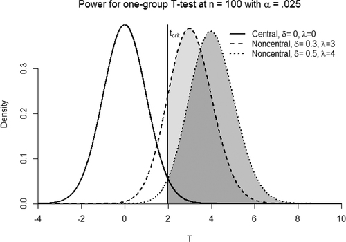
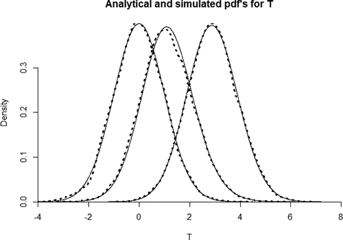
. As such, central sampling distributions are the ones we typically use in null-hypothesis tests, whereas non-central distributions are the ones needed to conduct a power analysis. To visualize what all of this means, depicts 3 Student
-distributions: one central
-distribution assuming that the null hypothesis is true, and 2 non-central distributions assuming that a given alternative hypothesis is true. Statistical power is represented by the area under the non-central distributions beyond the
.
Figure 1. Three T-distributions.
There are good reasons why statistical power is considered to be essential for a null hypothesis test. First, before conducting a study, we want to ensure a sample size that would give us a reasonable probability of rejecting the null if, in fact, the hypothesis of interest were true. If we know that there will be only a low probability of correctly rejecting the null hypothesis, there is little use to running the study at all! Second, high statistical power ensures that published null refutations will, on average, be more easily replicable and less inflated. This means that a literature relying on null hypothesis tests will be of more value if it is highly powered (Asendorpf et al., Citation2013). That being said, it should also be apparent that a consideration of statistical power still fails to address the most fundamental logical issue with tests of the null hypothesis: even though the sampling distribution under the hypothesis of interest is derived, the null hypothesis
is still the only one actually used for the statistical test. Fortunately, if we look at the statistical definition of power as in Expression (2), it is quite straightforward to arrive back at the definition of P-values as in Expression (1): we just need to plug in the observed test statistic
for
in Expression (1) to arrive at
-values in a strong-form set-up.
Practically speaking, though, this 'simple' extension will still raise questions: how could a communication scientist ever be able to define a substantive hypothesis for which a literal falsification would be theoretically meaningful? In contrast to physics, we do not have theories that allows us to derive point predictions, so setting up a test to falsify exactly
– as Meehl advocated – might seem out of reach. Fortunately, this problem has a practical solution: within the context of a power analysis, we will also rarely use a hypothesis derived from theory (even though that would be optimal); often, we will define the smallest effect size of interest (SESOI; Lakens et al., Citation2018) for which a we want a high probability of refuting the null (denoted by
). Of course, testing against a minimal effect size
does not exactly deliver the 'strongest' possible test in Meehl’s sense, which requires an exact theoretical point prediction
. However, it does give way for what at least appears to be a 'stronger' test than a typical nil-null test. That is, if we are able to define a meaningful
(ideally, based on a close reading of prior research findings or meta-analysis) we may also assess to what extent our findings serve as corroborating evidence that, in fact,
. To do so, we can evaluate the extremity of an observed test statistic
within the sampling distribution under the population parameter of minimal interest,
. This requires the calculation of a one-sided
-value, which we will denote by
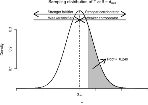
('P-dot'):Footnote6
As visualizes, represents the refutational information against the hypothesis of minimal interest that
(assuming
). When it is small, there is little refutational information against
(i.e., it is a corroborator of
); a high value for
implies a test statistic with considerable refutational information against the hypothesis that
(i.e., it is a falsifier of
. Synonymously, one could say that, in the former case,
entails falsifying information against
; in the latter case,
corroborates
.
Figure 2. Sampling distribution of -statistics given population effect sizes
is represented by the shaded area. The arrows show the direction and strength of corroborators and falsifiers.
Given this relatively straightforward extension from a typical (under the null) to
(under a hypothesis of minimal interest), it seems natural to ask: why has this approach not been adopted as a standard practice in the social-scientific literature? One reason could be that frequentist statistics has long been ritualized: the null routine has often been presented as “statistics per se” (Gigerenzer, Citation2004, p. 589), and even foundational principles such as statistical power took decades to be adequately considered (Cohen, Citation1992). A second reason could be that writings on strong-form testing have remained relatively scattered, operating under differing terminologies and, sometimes, lacking much technical and/or conceptual guidance. For instance, papers in the statistical reform movements have often been promoting the use of
-values under alternative, non-null-distributions, but they have not always attached conceptual or practical recommendations to it (Amrhein et al., Citation2019; Greenland, Citation2019; Nickerson, Citation2000). Others have provided more in-depth discussions on the relevant concepts and technicalities but discussed them within seemingly disparate frameworks. Some examples are minimal effects testing (Murphy & Myors, Citation1999), equivalency testing (Lakens et al., Citation2018; Weber & Popova, Citation2012; Wellek, Citation2010), magnitude-based inference (Aisbett et al., Citation2020), and severe testing (Mayo, Citation2018).
As the name suggests, minimal effects testing recommends an identical set-up to the one suggested in this paper (Murphy & Myors, Citation1999): define a minimal hypothesis of interest, derive the corresponding sampling distribution, and assess the extremity of an observed test statistic within this sampling distribution – that is, a quantity such as . Tests of equivalency are also technically similar, although the conceptual idea is somewhat different: within an equivalency test, researchers substantively predict the null-value, which requires them to (1) define the set of effect sizes that are 'practically equivalent' to the null and (2) refute the hypothesis that the population effect size is larger in absolute value than the upper and lower bounds of practical equivalence (Lakens et al., Citation2018; Weber & Popova, Citation2012; Wellek, Citation2010). This can be achieved on the basis of confidence intervals, or by calculating
-values from two one-sided tests against the largest effect size of practical equivalence ('TOST': Lakens et al., Citation2018). It should be clear that the latter is the same as setting up an estimate of
, deriving the non-central sampling distribution, and calculating
. Similar principles apply to the framework of magnitude-based inference, although one should be cautioned about the flawed, pseudo-Bayesian interpretations that have been circulating in this corner of the literature (see, Aisbett et al., Citation2020, for a discussion).
The most advanced philosophical treatment of strong-form testing has been delivered by Mayo (Citation2018). In Mayo’s terminology, 'strong testing' is referred to as 'severe testing'- more generally, 'error statistics' – but her basic argument is similar to Meehl’s (Citation1967). Mayo also emphasizes the falsificationist rationale of frequentist testing: as she puts it, the purpose of a statistical test should be to find out how severely the test probed a statistical hypothesis (e.g.,
) . To evaluate whether the hypothesis is severely probed we need to find out, first, how capable the test would have been to generate an observed test statistic as extreme as
if
had not been true. Technically, Mayo’s logic also boils down to (1) setting up the substantive hypothesis
, and (2) calculating the one-sided extremity of a test statistic
within a non-central sampling distribution assuming
. Mayo uses the concept of severity (
) to refer to the
-value-like quantity that arises from this, and
corresponds to what we have defined as
above: when
is low, there is a fairly low probability that
would have been larger than it is, if the population effect size would be any smaller or equal to
. By the Frequentist Principle of Evidence (Mayo & Spanos, Citation2006), this implies that the data are evidence that
. In contrast, when
is high, there is a fairly high probability that
would have been larger than it is if the population effect size had been at least
; by the Frequentist Principle of Evidence, this serves as counterevidence against
.
In this paper, we choose to stick to the symbol of rather than
because severe testing, as discussed by Mayo (Citation2018), entails much more than just the calculation of
-value-like quantities; for a claim to be severely tested researchers also need to probe the full chain of assumptions and auxiliaries underlying their tests (see also, Mayo, Citation2018; Scheel, Tiokhin, Isager, & Lakens, Citation2020; Spanos & Mayo, Citation2015). Here, we are only concerned with the calculation and interpretation of values such as
and
per se, so we prefer not to introduce the connotations attributed to the general concept of severe testing. Importantly, the fact that we are not concerned with probing model assumptions also entails an important caveat: throughout our discussion, we will already assume that all statistical assumptions for General Linear Models are met. If the model is incorrectly specified,
and
naturally lose their interpretability. That said, in all situations where we consider a regular
-value to be reasonably meaningful,
should also apply.
Strong-form frequentist testing: calculating  in the General Linear Model
Let us now turn to considering what communication scientists should do, specifically, to apply the principles of strong-form testing (aka, minimal effects testing, severe testing, etc.). To begin with, it should be clear from our previous discussion that the technical application is relatively straightforward for General Linear Models with fixed effects: much of the set-up of a strong-form test will remain identical compared to the typical null-hypothesis case: the type (i.e., ,
,
,
) and observed value of the test statistic will be the same, and the degrees of freedom will remain constant as well. This means that the information typically used and reported in a null-hypothesis test can be recycled into the calculation of
. The only technical challenge arises in deriving the non-centrality parameter
, which is needed to determine the sampling distribution of test statistics under the substantive hypothesis
.
The concept of the non-centrality parameter is rarely discussed in much detail in the literature on applied statistics. This is very surprising, especially given its fundamental role in power analyses; in fact, even Cohen’s (1988) widely cited reference manual on statistical power does not provide a lot of detail on the meaning or calculation of (see also, Liu & Raudenbush, Citation2004). Conceptually,
can be understood as a mathematical expression of “the degree to which the null hypothesis is false” (Kirk, Citation2013, p. 139). More technically, it is a parameter that arises in distributions of random variables that have been derived from other, normally distributed, random variables with non-zero means (Liu, Citation2014). It is these non-zero means of the initial variable that define the value of
for the newly defined random variable;
, in turn, can be factored into the expected value (the mean) of that new variable. The exact formula of
will depend on the underlying transformation, but it generally holds that
can be expressed as an increasing function of sample size
and population effect size
– i.e.,
, as noted above. We will not go into further detail on the derivation of
here; interested readers are referred to Liu (Citation2014) and the Technical Appendix (available from OSF, see https://osf.io/sdu9m/), where the origins of
are discussed further.
provides an overview of formulas of for common applications of the General Linear Model. Alongside the non-centrality parameter, also reports the formula for test statistics, degrees of freedom, and the functions that can be used to calculate
in R (R Core Team, Citation2020). Importantly, researchers do not necessarily need to calculate
manually through the formulas from ; any software application conducting power analyses for the General Linear Model should be able to determine
(as it is used behind the scenes anyway). G*Power (Faul, Erdfelder, Lang, & Buchner, Citation2007), for instance, routinely outputs whenever a researcher chooses a post-hoc power analysis procedure. To avoid confusion, this does not mean that a researcher using the post-hoc command in G*Power to calculate
will be conducting a post-hoc power analysis! In a post-hoc power analysis, one would use the observed effect size to calculate statistical power assuming that the observed effect size equals the population effect size. In contrast, when using G*Power to calculate
we only impute the smallest effect size of interest
into our calculation to obtain the value of
assuming that the population effect size were equal to the smallest effect size of interest. This set-up is clearly different, so there is no need to worry about the logical problems with post-hoc power analyses in the context of calculating
.
Table 1. Information needed to calculate in R for General Linear Models with fixed effects.
In sum, the practical workflow for calculating in General Linear Models will look something like this:
(1) Define the minimal effects size of interest prior to data collection. This is based on general insight in the research topic, previous research and literature review. Optionally, define (and pre-register) the cutoffs for the interpretation of statistics such as (see step 5).
(2) Conduct the nil-null hypothesis test (as one would usually do). The analysis outputs an observed test statistic and, when applicable, degrees of freedom, correlations between (repeated) measures, etc.
(3) Calculate the non-centrality parameter for the sampling distribution of test statistics. This can be done either through the formulas in or by choosing the ‘post-hoc’ procedure within G*Power and providing the necessary information (degrees of freedom, sample size, variances, minimal effect size of interest, correlations between repeated measures, …). Note that any value specified for α in software such as G*Power will be irrelevant for the calculation of λ.
(4) Use to choose the appropriate formula for calculating the the non-central Cumulative Distribution Function of T. Impute the observed test statistic t, the non-centrality parameter λ, and (when appropriate) degrees of freedom v as provided by steps 1 and 2. The outcome value, or its complement, generates (see ).
(5) Evaluate in terms of how much corroborating or falsifying evidence it provides for or against the claim
. When
is small, it offers (relatively speaking) more corroborating than falsifying information about
. When
is large, it offers (relatively speaking) more falsifying than corroborating information about
. How much falsifying or corroborating information one would need to consider it “convincing enough” will depend on the researcher’s testing philosophy and pre-registered cutoffs.
While this procedure is not overly complicated, steps 3 and 4 still require some manual operations. For this reason, a web application is being developed that allows researchers to automatically calculate based on the relevant inputs. A link to the application will be available on the OSF page associated with this project (https://osf.io/sdu9m).
Illustrative examples
We now turn to a discussion of three hypothetical examples to show how may be calculated and interpreted. The code associated with the examples is also available from OSF (https://osf.io/sdu9m/).
Example 1. Difference between two independent group means, unknown variances (equal variances assumed).
Imagine a researcher planning to conduct a simple advertising experiment with an independent two-group design: in one group, she will expose participants to an advertisement with celebrity endorsement; in the second group she will expose them to an advertisement with an unknown endorser. After exposure, she measures attitudes toward the product using a validated measurement scale. Say that she will be using a Student -test (assuming similar population variances in both groups) and predicts an effect size of minimal interest of at least
(a 'small' to 'medium' effect by Cohen’s standards). She wants to achieve reasonably high power – say,
– at a one-sided significance level of
(corresponding to the critical value of a two-sided
), which requires a total sample size
. She conducts the study and observes the mean attitude in the celebrity endorsement group to be 2.70 (
); in the control group it is 2.33 (
). This corresponds to an observed
, with
, and
(right-sided). This means (1) that the observation entails relatively strong falsifying evidence against the null hypothesis, and (2) that the observed effect size is larger than the effect size specified as being of minimal interest.
From the latter observation, it seems straightforward to conclude that, in fact, the findings corroborate . However, an important additional question is as follows: how strong is the corroborator? This can be evaluated on the basis of
. Plugging in the formulas from , the researcher finds that
corresponds to a non-centrality parameter
. She then applies the corresponding function in R – technically, the complement of the cumulative distribution function for the
-distribution:
). This results in
.
This can be interpreted in three equivalent ways. First, in terms of probability, this result means that there would be a probability of at least 9.3% to observe a larger test statistic than the one observed if the true population difference would be .30 or larger. Second, and more informally, the results suggest relatively strong counterevidence against . If
had been any smaller than
, the probability of finding a test statistic as large as the one observed would have been even smaller than
. This is identical to a third way of interpreting the results: the finding t serves as a relatively strong corroboration that
(see also ).
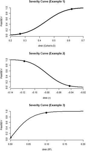
Figure 3. Distributions of and
belonging to examples 1, 2, and 3.
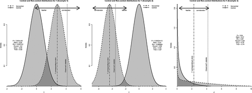
Example 2. A correlation coefficient.
Now consider a media researcher testing a traditional 'cultivation effects' hypothesis, suggesting there being a bivariate correlation between total television exposure and the expressions of beliefs in a just world (, second column). The researcher uses a large-scale survey in a random sample of 1900 adults, and observes . She concludes that the relationship is statistically significant at
and therefore corroborates the cultivation hypothesis. However, a reviewer posits that this is not at all convincing: while the finding provides refutational information against the null hypothesis, a theoretically meaningful manifestation of a cultivation effect should have a minimal effect size of at least
, or
. He notes that the observed effect size
already falsifies the claim – but how strong of a falsifier is it? The minimal effect size
implies
, which - according to - corresponds to non-centrality parameter
. Calculating
from this gives
. This means that the actual population effect size were no smaller (in absolute value) than a minimum effect size of interest
there would have been a probability of at least
to observe a larger test statistic (in absolute value) than the one we have observed. In other words, the observation serves as a relatively substantive falsifier with regard to a theoretically meaningful manifestation of a cultivation effect – even though the relationship is statistically significant by common standards.
Example 3. R2-change in multiple regression.
Consider the scenario where a student conducts a relatively small-scale survey () to assess the relationship between social media use and depressive feelings, measured using a validated measurement scale. The model also contains 4 socio-demographic and psychological variables as controls. The student hypothesizes that social media use contributes substantively to the explanation of variance in scores on the depression scale, reflected in a minimal change of
. Using a hierarchical regression she finds that the four control variables (added as a first block) generate
. In a second block, she adds social media use, which increases
by
. This means that, by the typical standards of a null hypothesis test, we would reject the null hypothesis and find an effect size of
, larger than one proposed as a minimal effect size of interest. Now, do we consider this finding as a strong corroborator of the hypothesis
? According to , the non-centrality parameter for
-change is given by
, and
is obtained through the cumulative distribution function of the
-distribution:
, which results in
. This does not seem fully convincing: there is still a
probability of observing a larger test statistic than the one observed if the population effect size would be at the absolute minimum value of interest
; that is, if the population effect size were any smaller than
, the probability of observing a larger test statistic would still only be at least
. Hence, the result lie in the direction of corroboration, albeit not convincingly.
Note from this example that the formula for used in multiple regression (i.e., based on
)is generalizable across tests within the General Linear Model: a relationship that can be expressed in terms of explained variance (i.e.,
or
) can be reformulated into the form of
. For ANOVA-type analyses, calculating
in this way will generally be easier than having to express all group-specific differences separately (see ).
The importance of interpreting overlap with the null distribution
Looking at the specifics of our third example, and comparing the curves from the three examples in , it should be clear that should not just be interpreted on the basis of the curve of the non-central distribution alone. That is, when the null and alternative distributions overlap heavily,
values will often be pointing into the direction of corroboration, even when the test statistics were drawn from the null distribution. To put it in falsificationist terms, a test with large overlap between the null and alternative distributions is highly unfalsifiable: even under the absolute null scenario, it would be relatively likely to find a tests statistic corroborating the hypothesis
. If the null and alternative distributions overlap completely, finding a corroborator for
is equally probable under
and
, which means that finding a corroboration is completely uninformative. This is a reminder that the interpretability of test results always depends, at the very least, on the results the test is expected to generate under absolute null scenario! A general rule is this: for any given
, a test with more overlap with the null distribution implies weaker corroborations of the claim
, as observations from the null distribution will be expected to generate relatively low
values with high probability (claim
is less falsifiable; cf., Mayo, Citation2018). This shows why evaluating
also always requires a consideration of overlap, distance, or divergence between the null distribution and the alternative distribution. There are several pieces of information that could be used as part of this evaluation.
A first piece of relevant information can be found by simply comparing the observed -value with
. When the two sampling distributions overlap completely,
and
for any given test statistic
will be identical. The less the two distributions overlap, the larger
should be compared to P for any given test statistic
. While this method is straightforward, it is also informal and subjective. More formal approaches will require the interpretation of statistics quantifying the overlap, distance, or divergence between the null and alternative distributions (see for a visualization). There are many options available, but we will focus our discussion on statistics with intuitive bounds between 0 and 1 (thereby excluding widely used statistics such as the Kolmogorov–Smirnov distance, the Kullback–Leibler divergence, and the Jensen-Shannon divergence).
One option is to evaluate statistical power of the null hypothesis test. Power has the advantage of being familiar to researchers, and it can be used as an indication of overlap in the sense that it is the probability of exceeding a critical (tail) value of the null distribution if the alternative is true. This may then lead one to conclude that, conceptually, higher power reflects higher distance and less overlap between the null and alternative distributions. The main problem with using power in this way is that it requires a significance level to be defined, which means that (1) it cannot be defined without requiring researchers to put a significance level in place, and (2) it is not comparable between different significance levels. These issues can be bypassed by extending the concept of power to what one could call “falsifiability.” “Falsifiability” can thus be defined as the probability of finding a test statistic that provides at least some falsifying information against if the null hypothesis were true. In other words, it corresponds to the probability of observing test statistics corresponding to
if the null hypothesis were true. Symbolically,
where (“phi”) stands for “falsifiability” (i.e., falsifiability of
when
), and
refers to the value of the test statistic corresponding to
. Falsifiability is conceptually similar to power, but instead of using probabilities under the alternative based on a critical value of
, it uses probabilities under the alternative based on the value of
corresponding to
. Hence, the value for
can easily be calculated through a minor extension of the test statistic formulas in : the expected effect size of interest
can be plugged into the formula for the test statistic, together with the observed sample size(s)
and (in case
is unstandardized) standard deviation(s)
. This will provide the test statistic corresponding to
From this, we can calculate the probability of observing test statistics smaller than
assuming that the null hypothesis is true. Ideally, this probability should be 1, as this means that
cannot be corroborated under the null hypothesis. Note that tests with reasonable power will already tend to spawn
very close to 1; this is important to keep in mind, because it means that one may set very high standards for
(with values nearing 1 being required).
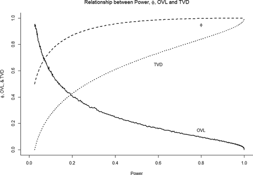
When comparing null and alternative distributions one may also resort to measures that have been specifically designed to quantify distributional (dis)similarity. One notable example of this is the so-called Overlapping Coefficient (), which is used as a similarity measure in various areas of statistics. OVL represents the percentual overlap of two distributions, meaning that it ranges from 0 (0% overlap) to 1 (100% overlap), with alues close to 0 to be preferred.
can be implemented in R using the Overlapping package (Pastore, Citation2018). As yet another alternative, one could calculate the Total Variation Distance (
), which is implemented in R through the distrEx package (Ruckdeschel et al., Citation2006).
also ranges from 0 to 1, and it represents the largest possible difference assigned to the same event by two probability distributions. If two distributions are identical, the largest possible difference in assigned probabilities is 0; if they are completely different (i.e., if they don’t overlap), the largest possible difference is 1. Hence, values close to 1 are also to be preferred here. illustrates the relationship of all statistics mentioned (power,
and
) in case of a two-sample
-test.
Figure 4. Graph representing the relationship between power, (“falsifiability”), the overlapping coefficient, and the total variation distance.
Now let us briefly consider how the overlap or distance between the alternative and null distributions would affect our interpretation of our three examples. Eyeballing , it is clear that the curves from the third example overlap heavily, whereas the curves of the other two examples do not: in the first and second example, there is relatively high power, little overlap and high falsifiability. In the third example, however, the distributions under the null and substantive hypothesis overlap heavily, which is also reflected in the values of power, ,
, and
. Considering
specifically, the third example shows a
probability of finding a test statistic in the direction of
if the null hypothesis is true. In other words, this still leaves a.13 probability of corroborating
if, in reality,
. The values of
are close to 1 for the other two examples, showing that, comparatively, they provide more informative and adequate tests. Note that the web application associated with this article will also include an option to output these measures of overlap and similarity alongside
(see https://osf.io/sdu9m).
What about the overlap with other, non-null-distributions?
There is an infinite set of possible parameter values different from , all of which would spawn a different value for
, a different sampling distribution, and a different value for
. One could ask: should a researcher not evaluate all of these parameters? Our answer would be: no, not necessarily. We know that testing any effect below
would always suggest more corroborating information in test statistic
. But given that we were calculating
at the minimal effect size of interest, any
is not of relevance. Likewise, a given
will always generate less corroborating information for effect sizes larger than
, but this is also not much of an issue for the initial hypothesis test: the only claim we are making is that
, so finding less corroborating information for any alternative
has no direct implications for our claim.
Importantly, this is not to say that it is irrelevant to evaluate the falsifying or corroborating information of an observed test statistic in light of parameter values other than
. However, doing so seems of most use after the initial hypothesis test of interest – that is, as a follow-up, 'inductive' step. We see two ways in which a researcher could proceed at this stage. A first approach is to evaluate confidence intervals for an observed effect size. In recent years, the reporting of confidence intervals for effect sizes has been widely promoted, even to the extent that it has been dubbed “the new statistics,” ready to replace
-values (Cumming, Citation2014, p. 7). From the viewpoints expressed in this paper, confidence intervals should not be seen as a replacement of
-like quantities. Rather, we believe they are mutually compatible, of use at subsequent steps of the testing-and-inference-cycle: we first test a hypothesis of minimal interest, and then we may use confidence intervals to infer the range of parameter values that could not be rejected (at a fixed
level). That is, confidence intervals represent intervals of non-refutation (corroboration) given an observed test statistic
and dichotomous decision rule (i.e., corroborate/falsify) based on some threshold
(“compatibility intervals”: Amrhein et al., Citation2019; Greenland, Citation2019; Hawkins & Samuels, Citation2021). A second approach – and one that does not require fixed α levels – is to eyeball so-called “severity curves” (Mayo, Citation2018). Severity curves represent the value of
, or
, for a wide range of parameter values. Plotting severity curves can be done iteratively, through a simple application of the formulas in . The steps are as follows: (1) specify a range of values for the hypothesized effect size, (2) calculating
given all of these effect sizes, and (3) plot the values for
against their respective effect sizes. shows severity curves for the three examples described above. The accompanying web application will also include the option to plot severity curves automatically (see https://osf.io/sdu9m).
Figure 5. Severity curves for the three examples.
Summary: the steps in a ‘strong-form’ test
In sum, there will typically be four practical steps associated with a ‘strong-form’ test:
Define minimal effect size of interest
Calculate a traditional P-value. Critically evaluate the extent to which it corroborates or falsifies
Calculate
Evaluate the overlap, distance, or divergence between the alternative and null distributions. A corroboration should be considered as (relatively) less valuable when there is a large overlap, and (relatively) more valuable when there is little overlap.
Assess the corroborating/falsifying information in
The behavior of : a simulation
We now turn to a simulation to illustrate our previous claims and to portray the long-term behavior of and
in more detail. The simulations revolve around the example of a correlation coefficient, but the definition of standardized quantities such as
and
does not depend on the type of statistic being used. As a result, the general pattern of findings shown here will extend to other types of statistics as well – at least as long as the assumptions of the underlying statistical models are met.
Set-up
In our simulation, we begin by defining five population effect sizes for the correlation coefficient , five sample sizes
, five hypothesized (i.e.,
) correlations that are supposedly put to the test
, and one significance level of
(one-tailed). For all combinations, we simulate 10,000 data sets and store observed test statistics,
-values,
-values, non-centrality-parameters (
), and measures of similarity or overlap. This allows us to simulate the behavior of
and
(1) under various combinations of true effect sizes, tested effect sizes, and sample sizes, and (2) under various conditions of the overlap between the null and alternative distributions. The annotated code of the simulation is available from the paper’s OSF repository (https://osf.io/sdu9m/).
Illustration of key points
The non-centrality parameter is an increasing function of sample size and population effect size, so the distribution of simulated test statistics should shift further away from zero the higher (1) the population value of the correlation coefficient, and (2) the sample size. As visualized by , this is reflected in the simulations: when the population correlation coefficient
, the simulated distribution of test statistics follows a central distribution with
. When the population coefficient is non-zero, the distribution of observed test statistics shifts to a non-central
distribution with
.
Figure 6. Analytical and simulated pdf’s for .
Of course, in reality, researchers will always be working with sampling distributions under a hypothesized effect size, and not the true effect size. This means that when we are calculating or
(i.e., under a hypothesized effect of 0 or
) we are assuming a distribution that may or may not differ from the true distribution. The distribution of
and
values will therefore also depend on the difference between the hypothesized and actual sampling distributions of test statistics. To illustrate, consider the case of a regular
-value, where the hypothesized effect size is always equal to
. It is a well-known fact that, if the null hypothesis is true (if
), P-values will be uniformly distributed between 0 and 1 – regardless of sample size. This follows directly from the definition of a
-value, which can be interpreted as stating that, if the null hypothesis were true, the observed test statistic
would be at the
th percentile of highest ranked test statistics. From this it follows that if the null hypothesis is actually true, exactly
percent of all test statistics will result in a
-value smaller than
; that is,
, which implies a uniform distribution. In contrast, if the true population effect size is any greater than 0, P will have a right-skewed distribution. This also makes sense: if we are drawing test statistics from a distribution that, on average, spawns large tests statistics, then we will, on average, find small P-values. This phenomenon will be more and more pronounced the more the true non-centrality parameter
moves away from 0 (that is when the effect size and/or sample sizes increase). This behavior of
-values is visualized in .
Figure 7. The sampling distribution of under varying population effect sizes and sample sizes (upper figure), and the sampling distribution of
under varying population effect sizes and sample sizes (lower figure).
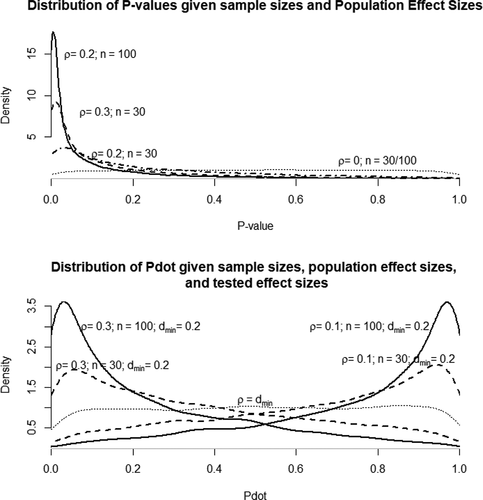
Unsurprisingly, the behavior of P also translates into ;
will also be uniformly distributed if the tested hypothesis
is true in reality, and if the true effect size is larger (in absolute value) than the tested parameter
, the sampling distribution of
will be right-skewed as well. However, as shows, there is another interesting case to consider for
: if the true effect size is smaller than the hypothesized effect
the sampling distribution will be left-skewed. This means that for a population parameter greater than 0 but smaller than
, the distribution of
will be right-skewed, and the distribution of
will be left-skewed. The skew in the distribution of
will also more pronounced when the true non-centrality parameter diverges to a greater extent from the one assumed in the hypothesis test (e.g., when the population effect size differs greatly from the tested effect size).
The notion of skew in distributions illustrates two fundamental points about the interpretation of strong-form tests. First, it illustrates the importance of sample size: for any fixed population effect size and tested effect size, it will be true that with increasing sample sizes, it will be easier to find falsifiers against the hypothesis
if the population effect size were any smaller than the tested effect
. This means that higher sample sizes increase Popperian ‘risk’ (Meehl, 1968): there is a higher probability of refutation of a hypothesis
if, in reality,
is somewhat smaller than
. Likewise, higher sample sizes will also make it easier to detect strong corroborators if the actual population effect size were any greater than
. Both of these indicate why researchers would want to aim for large samples: (1) larger samples increase falsifiability and should therefore be lauded by reviewers; (2) when
is any greater than
, higher sample sizes will, on average, spawn smaller values of
(i.e., the results will tend to be more convincing).
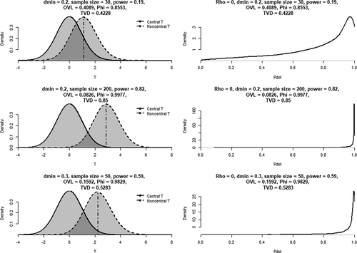
A second crucial point illustrated by the skew in the distribution of is the relevance of (dis)similarity and overlap between the null and alternative distributions: when sample sizes and/or effect sizes are very small (i.e., when non-centrality parameters are very small) the null and alternative distributions overlap heavily. When this is the case
will, on average, be smaller under the null hypothesis, and, as a result, become less informative: even if the absolute null situation were true, it would be relatively likely to find strong corroborating information that
. This is also reflected in the distribution of
-values: the more the distributions overlap, the less the distribution of
will be skewed if the null hypothesis is true – that is, the higher the probability becomes of finding small
-values under the null. To illustrate, visualizes the distribution of
-values at various levels of overlap with the null distribution, quantified by (1) power, (2)
, (3)
, and (4)
.
Figure 8. The effects of and sample size (left column) on (1) the overlap between central and non-central distributions (left and middle column), and (2) the distribution of
if the null hypothesis is true (right column).
The added value of the strong-form construal
In our view, the construal of strong-form frequentist testing (severe testing, minimal effects testing, etc.) offers a promising addition to the statistical toolbox of communication scientists. It is a relatively straightforward extension of widespread practice, and it adds to the convergent evolution of the field toward critical theory assessment in a falsificationist sense: a strong-form test allows for a more direct evaluation of a statistical hypothesis, requires a more critical reading of findings that are “statistically significant,” and underlines the importance of making thoughtful methodological decisions before conducting a study. That is, if we require strong-form tests (or some related conceptualization), researchers will need to pre-register a reasonable value for on the basis of their knowledge of the literature (see also, Dienlin et al., Citation2020). Fixing one general value of
across studies will not be very useful, as the effect size of interest will be highly contingent on the type of hypothesis under investigation. For instance, when a researcher is conducting a large-scale survey to assess the overall relationship between media use and well-being it seems reasonable to set
to a relatively low value. In contrast, when the purpose of a study is to test the behavioral effects of a costly intervention campaign, it will be necessary to specify a much larger effect size as being of minimal interest. For this reason, the specification of a given
should be considered as a central topic of both a study’s pre-registration plan as well as its literature review. In general, and when feasible, larger values of
are to be preferred as they represent more meaningful effects in a theoretical and practical sense; methodologically, they generate less overlap between the null and alternative distribution given a fixed sample size (i.e., higher falsifiability).
Another advantage of the strong-form construal is that it incentivizes researchers to gather large samples. This incentive is much more apparent compared to the traditional null hypothesis -value, because it literally creeps into our interpretation of ‘evidence’: if we only gather small samples we know that, when evaluating the results, we will find larger overlap between the null and alternative distributions. As a result, a corroborator (if we already find one) will be considered of less value than it would have been if we had had a larger sample. Also, the larger the sample size, the smaller
will be for relatively small deviations
. This means that larger sample sizes will make it easier to find corroborating information in favor of
if, in reality, the population parameter is any greater than
. Hence, gathering larger samples will generally be more interesting for researchers and, at the same time, ensure a more risky test of hypotheses. In other words, in a strong-form set-up, gathering large samples will be a win–win situation for both science and the scientist (which is not necessarily the case for null hypothesis tests, where scientifically meaningless deviations from 0 already spawn low
-values with large samples).
A third advantage of strong-form testing is that it underlines the value of oft-maligned distance measures such as , up and above confidence intervals (Cumming, Citation2014): when assessing the falsifying information of a finding in light of a fixed hypothesis, confidence intervals only provide binary information about a predicted parameter – that is, it lies within the interval or not. Distance measures are more specifically informative, as they quantify the extremity of an observation against a specific prediction. As we have mentioned earlier, measures such as
or
and confidence intervals can be seen as complementary: we first test predictions by evaluating falsifying information as expressed through a distance measure; next, we may use an interval to (inductively) reason through the set of hypothetical parameter values for which the observation would not be among the
most extreme observations. Alternatively, if we are unwilling to specify a given significance level, we may use severity curves to obtain an overview of Ṗ values across hypothetical parameter values.
Challenges, limitations and future directions
Despite its potential for strengthening the statistical inferences of communication scientists, the strong-form framework carries along various challenges. Most crucially, it is in need of a generally established set of definitions and best-practices: as there are still many ways to define or conceptualize similar sets of ideas, researchers will need to add some technical detail to their statistical definitions and calculations when resorting to strong-form tests. While this might raise the bar for practically oriented scholars, we hope that the principles laid out in this paper are formulated clearly enough to be used as a reference guide.
A second challenge is finding a way to generalize the principles of strong-form testing to more complicated analyses. By this, we mainly refer to situations where the non-centrality parameter is not easily expressed in terms of standardized effect sizes, and/or the sampling distribution cannot be derived analytically. With regard to the first situation, it might happen that we are unable (or unwilling) to express effects sizes in standardized form: some methodologists have argued against the use of standardized metrics (e.g., Baguley, Citation2009) and, in some situations, there is no consensus on how a standardized effect should be defined at all (e.g., when variances are not assumed to be homogeneous, as in a Welch ANOVA). Under these circumstances, calculating the non-centrality parameter will often require us to separately define (1) raw effect sizes as well as (2) population variances. Of course, population variances are typically unknown, so the only way to proceed seems to be with using the sample variance to calculate the non-centrality parameter. This is not unreasonable – the sample variance is, after all, an unbiased estimator – but it does introduce an additional layer of variability: the sample variance has its own sampling distribution and may therefore generate both an under- or overestimation of the true population variance. The key question therefore is as follows: what would this use of a sample variance imply, exactly, for the conclusions drawn from a statistic such as Ṗ? Detailing the answer to this question goes beyond the scope of the current paper, and we leave a full discussion to future studies. However, it seems that there are at least two competing dynamics to be considered: on the one hand, the sample variance will underestimate the population variance more than 50% of the time (its distribution is right-skewed). This means that, more often than not, the non-centrality parameter calculated through the sample variance will be greater than the non-centrality parameter obtained through the population variance. As a consequence, the overlap between the null and alternative distributions will be underestimated more than 50% of the time when using the sample variance, and quantities such as statistical power will be overestimated more than 50% of the time. On the other hand, as we know that Ṗ will be calculated on the basis of a non-centrality parameter that is, on average, overestimated, Ṗ should typically be overly conservative: that is, a given test statistic will, relatively speaking, generate a higher Ṗ value (less corroborative information for ) than it would have had if we had used the population variance to calculate the noncentrality parameter. This would appear to provide yet-another incentive for researchers to obtain high sample sizes: with higher sample sizes, Ṗ as calculated from sample variances would be underestimated less often.Footnote7
Another complication for strong-form testing arises when non-central distributions are not easily expressed in analytical form. This occurs, for instance, for the widely used cases of logistic regression, multilevel models, and structural equation models. For logistic regression – which is a non-linear model – we need to consider that alternative distributions of the test statistic are contingent on the exact distribution of the independent variables (Demidenko, Citation2007); for multilevel models we need to specify separate variance components (Snijders, Citation2005); and for SEM we naturally need to take into account measurement reliabilities (Liu, Citation2014). While there are workarounds to approximate these non-central distributions without changing much to the principles for the General Linear Model (see Faul et al., Citation2009, for logistic regression, or Liu, Citation2014, for multilevel models and SEM) it seems useful to think about developing a framework for strong-form testing that does not require analytical solutions. For instance, one could consider extending the strong-testing framework to simulation-based methods which is, in fact, the way in which frequentist testing proceeds in physics or how power analyses are set up for complicated use-cases. A detailed treatment or validation of simulation-based applications is far beyond the scope of the present paper, so future studies should flesh out those principles in more detail. We believe, however, that this exercise would be particularly useful: a generalizable framework for strong-form testing would not just add to the statistical practices of communication scientists, but it could aid all of the social sciences evolve toward a common standard for critical hypothesis testing.
With all of this said, there is still one important caveat to be stressed: conducting what we called strong-form tests should not be conflated with ‘having strong theories.’ Strong-form testing makes a more stringent assessment of theoretical claims possible – at least compared to nil-null testing – but it provides no safeguard against testing theoretically meaningless (or methodologically contrived) claims. Hence, communication scientists should be wary not to overinterpret the results of a strong-form test – or any test, for that matter. A qualitative appraisal of theoretical arguments and methodological choices remains essential, regardless of the value obtained for any summary statistic such as P or Ṗ.
Supplemental Material
Download ()Disclosure statement
No potential conflict of interest was reported by the author(s).
Supplementary material
Supplemental materials (code and technical appendix) for this article can be accessed online at https://doi.org/10.17605/OSF.IO/SDU9M
Additional information
Funding
Notes on contributors
Lennert Coenen
Lennert Coenen (PhD, KU Leuven) is an assistant professor at the Tilburg Center for Cognition & Communication (Tilburg University, The Netherlands) and a visiting professor at the Leuven School for Mass Communication Research (KU Leuven, Belgium). His research mainly aims to develop theory, metatheory, and methodology in the area of media effects on public opinion.
Tim Smits
Tim Smits (PhD, KU Leuven) is a full professor in Persuasion and Marketing Communication at the institute for Media Studies, KU Leuven, Belgium. Tim published on various topics within these fields, but his main research focus pertains to persuasion and marketing communication dynamics that involve health and/or consumer empowerment and how these are affected by situational differences or manipulations. He also has a more methodological line of research on science replicability.
Notes
1 For the sake of simplicity of these expressions we assume throughout the paper, unless stated otherwise.
2 Most texts would prefer to instead of
. When talking about continuous distributions (as we will be doing throughout the paper) this is the same thing: the probability at any single point in a continuous distribution is
. Thus,
.
3 Important arguments against interpreting -like quantities in terms of (counter)evidence are (1) that
does not directly say anything about the truth or falsity of a hypothesis; (2) that all
-values are equally likely under the null hypothesis; (3) that, under conditions of low power, relatively high
-values do not provide any evidence against a null hypothesis; and (4) that, under conditions of high power, relatively low
-values may actually provide more evidence in favor of the null rather than an alternative. The current paper takes note of these concerns: for (1), it will be stressed that
-values provide information about the extremity of an observation assuming the truth of a hypothesis. Thus,
is only used to quantify the observation; when extreme, the observation is considered to be a falsifier of the hypothesis (but this doesn’t mean the hypothesis has been shown to be false; see also Footnote 4). For (2), it will be noted that, under any alternative hypothesis
,
-values nearing 0 are more likely (assuming
). This is reflected in our discussion on the skewed distribution of
- and
-values; the skew, then, is taken to be suggestive of the direction of δ compared to 0 or, more generally, d (i.e., whether the finding is a falsifier or corroborator). For (3) and (4), it will be stressed that any interpretation of a
- or
-value requires an explicit consideration of other metrics such as statistical power (i.e., the overlap between null and alternative distributions).
4 Note that we are actually cutting a terminological corner in this paper in order not to overcomplicate our discussion: it is very typical to say, as we have said here, that when , the tested hypothesis can be rejected. However, there is a subtle problem in this wording, as it conflates a property of the observation (i.e.,
is extreme enough to be called a falsifier of a hypothesis) with a property of the hypothesis (i.e., the hypothesis is falsified). Generally, in a frequentist framework – and in contrast with a Bayesian approach – we do not actually try to falsify or confirm any given hypothesis. That is, the focus lies on calculating the probability of observations assuming the truth of a hypothesis
theore – not on the probability of a hypothesis conditioned on the observations,
. Strictly speaking, then, in frequentist terms
does not allow us to say that “the tested hypothesis can be rejected”. Rather, it suggests that the test statistic is extreme enough to be called “a falsifying observation with regard to the hypothesis”. Similarly,
should not be defined as “the probability of a false refutation”, but rather as “the probability of incorrectly labelling an observation as a falsifier”.
5 An in-depth treatment of Bayesian inference is not within the scope of this paper; interested readers are referred to Gelman et al., Citation2013).
6 The way in which is defined here would traditionally be said to correspond to a one-sided test of the form
rather than a test of the form
. Therefore, this definition might not appear to be formally consistent with our requirement of putting the actual hypothesis
to the test. However, we prefer to stick with this definition for two reasons. (1) The tests of
and
are statistically identical for continuous distributions of
, in the sense that both tests evaluate
at
. This means that
-values arising from both set-ups provide the exact same information (they are just each other’s complement). (2) If we would have defined
as formally expected, a researcher would have needed to use inverse logic when interpreting
and
. That is, a low
-value typically means falsifying
(i.e., it is in line with a substantive claim; ‘good’!), but a low
would have meant ‘falsifying
(i.e., not in line with the substantive claim; ‘bad!’). In our definition,
and
values maintain the same evidential rank-order. Yet another possibility would have been to also define traditional
-values as testing the hypothesis
. This would also have maintained the rank-order compared to testing the claim
but it would have inverted the interpretation of traditional
-values: instead of ‘smaller is better’ it would be ‘larger is better’. This, we think, would have been unnecessarily confusing for researchers used to work with
-values.
7 All of this being said, initial simulations suggest that over- and underestimation of the population variance will occur with almost equal probability when errors are normal and sample sizes are reasonably large.
References
- Aisbett, J., Lakens, D., & Sainani, K. (2020). Magnitude based inference in 23Relation to one-sided hypotheses testing procedures. SportRχiv. https://doi.org/10.31236/osf.io/pn9s3
- Amrhein, V., & Greenland, S. (2017). Remove, rather than redefine, statistical significance. Nature Human Behaviour, 2(1), 4–4. https://doi.org/10.1038/s41562-017-0224-0
- Amrhein, V., & Greenland, S. (2018). Remove, rather than redefine, statistical significance. Nature Human Behaviour, 2(1), 4. https://doi.org/10.1038/s41562-017-0224-0
- Amrhein, V., Trafimow, D., & Greenland, S. (2019). Inferential statistics as descriptive statistics: There is no replication crisis if we don’t expect replication. The American Statistician, 73(sup1), 262–270. https://doi.org/10.1080/00031305.2018.1543137
- Asendorpf, J. B., Conner, M., de Fruyt, F., de Houwer, J., Denissen, J. J. A., Fiedler, K., … Wicherts, J. M. (2013). Recommendations for increasing replicability in psychology. European Journal of Personality, 27(2), 108–119. https://doi.org/10.1002/per.1919
- Baguley, T. (2009). Standardized or simple effect size: What should be reported? British Journal of Psychology, 100(3), 603–617. https://doi.org/10.1348/000712608X377117
- Benjamin, D. J., Berger, J. O., Johannesson, M., Nosek, B. A., Wagenmakers, E. J., Berk, R., Bollen, K. A., Brembs, B., Brown, L., Camerer, C., & Cesarini, D. (2018). Redefine statistical significance. Nature Human Behaviour, 2(1), 6–10. https://doi.org/10.1038/s41562-017-0189-z
- Cohen, J. (1988). Statistical Power Analysis for the Behavioral Sciences. Hillsdale, NJ: Erlbaum.
- Cohen, J. (1992). A power primer. Psychological Bulletin, 112(1), 155. https://doi.org/10.1037/0033-2909.112.1.155
- Cousins, R. D. (2020). Connections between statistical practice in elementary particle physics and the severity concept as discussed in Mayo’s Statistical Inference as Severe Testing. ArXiv:2002.09713 [Hep-Ex, Physics:Physics, Stat]. http://arxiv.org/abs/2002.09713
- Cumming, G. (2013). Cohen’s d needs to be readily interpretable: Comment on Shieh (2013). Behavior Research Methods, 45(4), 968–971. https://doi.org/10.3758/s13428-013-0392-4
- Cumming, G. (2014). The new statistics: Why and How. Psychological Science, 25(1), 7–29. https://doi.org/10.1177/0956797613504966
- De Groot, A. (1956/2014). The meaning of “significance” for different types of research (translated and annotated by Eric-Jan Wagenmakers, Denny Borsboom, Josine Verhagen, Rogier Kievit, Marjan Bakker, Angelique Cramer, Dora Matzke, Don Mellenbergh, and Han LJ van der Maas). Acta Psychologica, 148, 188–194.https://doi.org/10.1016/j.actpsy.2014.02.001
- Demidenko, E. (2007). Sample size determination for logistic regression revisited. Statistics In Medicine, 26(18), 3385–3397. https://doi.org/10.1002/sim.2771
- Derksen, M. (2019). Putting Popper to work. Theory & Psychology, 29(4), 449–465. https://doi.org/10.1177/0959354319838343
- Dienlin, T., Johannes, N., Bowman, N. D., Masur, P. K., Engesser, S., Kümpel, A. S., Lukito, J., Bier, L. M., Zhang, R., Johnson, B. K., Huskey, R., Schneider, F. M., Breuer, J., Parry, D. A., Vermeulen, I., Fisher, J. T., Banks, J., Weber, R., Ellis, D. A., & de Vreese, C. (2020). An Agenda for open science in communication. Journal of Communication, 71(1), 1–26. https://doi.org/10.1093/joc/jqz052
- Faul, F., Erdfelder, E., Lang, A., & Buchner, A. (2007). G*power 3: A flexible statistical power analysis program for the social, behavioral, and biomedical sciences. Behavior Research Methods, 39(2), 175–191. https://doi.org/10.3758/bf03193146
- Faul, F., Erdfelder, E., Buchner, A., & Lang, A.-G. (2009). Statistical power analyses using G*Power 3.1: Tests for correlation and regression analyses. Behavior Research Methods, 41(4), 1149–1160. https://doi.org/10.3758/BRM.41.4.1149
- Fisher, R. (1955). Statistical methods and scientific induction. Journal of the Royal Statistical Society: Series B (Methodological), 17(1), 69–78. https://doi.org/10.1111/j.2517-6161.1955.tb00180.x
- Gelman, A., Carlin, J. B., Stern, H. S., Dunson, D. B., Vehtari, A., & Rubin, D. B. (2013). Bayesian data analysis (3rd ed.). Chapman & Hall/CRC.
- Gigerenzer, G. (2004). Mindless statistics. The Journal of Socio-Economics, 33(5), 587–606. https://doi.org/10.1016/j.socec.2004.09.033
- Greenland, S., Senn, S. J., Rothman, K. J., Carlin, J. B., Poole, C., Goodman, S. N., & Altman, D. G. (2016). Statistical tests, P values, confidence intervals, and power: A guide to misinterpretations. European Journal of Epidemiology, 31(4), 337–350. https://doi.org/10.1007/s10654-016-0149-3
- Greenland, S. (2019). Valid p-values behave exactly as they should: Some misleading criticisms of p-values and their resolution with s-values. The American Statistician, 73(sup1), 106–114. https://doi.org/10.1080/00031305.2018.1529625
- Haig, B. D. (2020). What can psychology’s statistics reformers learn from the error-statistical perspective? Methods in Psychology, 2, 100020. https://doi.org/10.1016/j.metip.2020.100020
- Hawkins, A. T., & Samuels, L. R. (2021). Use of confidence intervals in interpreting nonstatistically significant results. JAMA, 326(20), 2068–2069. https://doi.org/10.1001/jama.2021.16172
- Kirk, R. E. (2013). Experimental design: Procedures for the behavioral sciences (4th ed.). Sage Publications, Inc.
- Lakatos, I. (1978). Falsification and the methodology of scientific research programmes. In J. Worrall & G. Currie (Eds.), The methodology of scientific research programmes: Philosophical papers (Vol. 1, pp. 8–101). Cambridge University Press.
- Lakens, D., Adolfi, F. G., Albers, C. J., Anvari, F., Apps, M. A. J., Argamon, S. F., Baguley, T., Becker, R. B., Benning, S. D., Bradford, D. E., Buchanan, E. M., Caldwell, A. R., Van Calster, B., Carlsson, R., Chen, S., Chung, B., Colling, L. J., Collins, G. S., Crook, Z., & Zwaan, R. A. (2018). Justify your α. Nature Human Behavior, 2(3), 168–171. https://doi.org/10.1038/s41562-018-0311-x
- Lakens, D. (2021). The practical alternative to the P value is the correctly used P value. Perspectives on Psychological Science, 16(3), 639–648. https://doi.org/10.1177/1745691620958012
- Levine, T. R., Weber, R., Hullett, C., Park, H. S., & Lindsey, L. L. M. (2008). A Critical Assessment of Null Hypothesis Significance Testing in Quantitative Communication Research. Human Communication Research, 34(2), 171–187. https://doi.org/10.1111/j.1468-2958.2008.00317.x
- Liu, X., & Raudenbush, S. (2004). A note on the noncentrality parameter and effect size estimates for the F test in ANOVA. Journal of Educational and Behavioral Statistics, 29(2), 251–255. https://doi.org/10.3102/10769986029002251
- Liu, X. S. (2014). Statistical power analysis for the social and behavioral sciences: Basic and advanced techniques. Routledge.
- Mayo, D. G., & Spanos, A. (2006). Severe testing as a basic concept in a Neyman–Pearson philosophy of induction. The British Journal for the Philosophy of Science, 57(2), 323–357. https://doi.org/10.1093/bjps/axl003
- Mayo, D. (2018). Statistical inference as severe testing. How to get beyond the statistics wars. Cambridge University Press.
- Mayo, D. (2019). P -value thresholds: Forfeit at your Peril. European Journal of Clinical Investigation, 49(10), e13170. https://doi.org/10.1111/eci.13170
- McShane, B. B., Gal, D., Gelman, A., Robert, C., & Tackett, J. L. (2019). Abandon statistical significance. The American Statistician, 73(sup1), 235–245. https://doi.org/10.1080/00031305.2018.1527253
- Meehl, P. E. (1967). Theory-Testing in psychology and physics: A methodological paradox. Philosophy of Science, 34(2), 103–115. https://doi.org/10.1086/288135
- Meehl, P. E. (1990). Appraising and amending theories: The strategy of lakatosian defense and two principles that warrant it. Psychological Inquiry, 1(2), 108–141. https://doi.org/10.1207/s15327965pli0102_1
- Murphy, K. R., & Myors, B. (1999). Testing the hypothesis that treatments have negligible effects: Minimum-effect tests in the general linear model. The Journal of Applied Psychology, 84(2), 234–248. https://doi.org/10.1037/0021-9010.84.2.234
- Neyman, J. (1942). Basic ideas and some recent results of the theory of testing statistical hypotheses. Journal of the Royal Statistical Society, 105(4), 292–327. https://doi.org/10.2307/2980436
- Nickerson, R. S. (2000). Null hypothesis significance testing: A review of an old and continuing controversy. Psychological Methods, 5(2), 241–301. https://doi.org/10.1037/1082-989x.5.2.241
- PASS. (2020). Power analysis and sample size software [Computer Software]. NCSS, LLC. ncss.com/software/pass
- Pastore, M. (2018). Overlapping: A R package for estimating overlapping in empirical distributions. Journal of Open Source Software, 3(32), 1023. https://doi.org/10.21105/joss.01023
- Popper, K. (1963). Conjectures and refutations: The growth of scientific knowledge. Routledge and Kegan Paul.
- R Core Team (2020). R: A language and environment for statistical computing. https://www.R-project.org/
- Ruckdeschel, P., Kohl, M., Stabla, T., & Camphausen, F. (2006). S4 classes for distributions. R News, 6(2), 2–6. https://cran.r-project.org/web/packages/distrDoc/vignettes/distr.pdf
- Scheel, A. M., Tiokhin, L., Isager, P. M., & Lakens, D. (2020). Why hypothesis testers should spend less time testing hypotheses. Perspectives on Psychological Science, 16(4), 744–755. https://doi.org/10.1177/1745691620966795
- Snijders, T. A. B. (2005). Power and sample size in multilevel linear models. In B. S. Everitt & D. C. Howell (Eds.), Encyclopedia of statistics in behavioral science (Vol. 3, pp. 1570–1573). Wiley.
- Spanos, A. (2014). Recurring controversies about P values and confidence intervals revisited. Ecology, 95(3), 645–651. https://doi.org/10.1890/13-1291.1
- Spanos, A., & Mayo, D. G. (2015). Error statistical modeling and inference: Where methodology meets ontology. Synthese, 192(11), 3533–3555. https://doi.org/10.1007/s11229-015-0744-y
- Vermeulen, I., Beukeboom, C. J., Batenburg, A., Avramiea, A., Stoyanov, D., van de Velde, B., & Oegema, D. (2015). Blinded by the light: How a focus on statistical “Significance” may cause p-value misreporting and an excess of p-values just below.05 in communication science. Communication Methods and Measures, 9(4), 253–279. https://doi.org/10.1080/19312458.2015.1096333
- Wasserstein, R. L., Schirm, A. L., & Lazar, N. A. (2019). Moving to a world beyond “ p < .05. The American Statistician, 73(sup1), 1–19. https://doi.org/10.1080/00031305.2019.1583913
- Weber, R., & Popova, L. (2012). Testing equivalence in communication research: Theory and application. Communication Methods and Measures, 6(3), 190–213. https://doi.org/10.1080/19312458.2012.703834
- Wellek, S. (2010). Testing statistical hypotheses of equivalence and noninferiority (2nd ed.). CRC Press.