How to resolve microsecond current fluctuations in single ion channels: The power of beta distributions

Abstract

A main ingredient for the understanding of structure/function correlates of ion channels is the quantitative description of single-channel gating and conductance. However, a wealth of information provided from fast current fluctuations beyond the temporal resolution of the recording system is often ignored, even though it is close to the time window accessible to molecular dynamics simulations. This kind of current fluctuations provide a special technical challenge, because individual opening/closing or blocking/unblocking events cannot be resolved, and the resulting averaging over undetected events decreases the single-channel current. Here, I briefly summarize the history of fast-current fluctuation analysis and focus on the so-called “beta distributions.” This tool exploits characteristics of current fluctuation-induced excess noise on the current amplitude histograms to reconstruct the true single-channel current and kinetic parameters. A guideline for the analysis and recent applications demonstrate that a construction of theoretical beta distributions by Markov Model simulations offers maximum flexibility as compared to analytical solutions.

Keywords:

• β
• distribution
• fast block
• fast current fluctuations
• fast gating
• flickery gating
• open-channel noise
• rate constants
• skewed amplitude histogram
• true single-channel current

Introduction

Understanding structure/function correlates in ion channels

Ion channels are key players in both excitable and in non-excitable cells. They are instrumental to the function of neurons and muscles,^1-3 they control the rate of the heart beat^4,5 and multiple steps in cell development.⁶ Thus, the question of how the structure of a channel protein determines its function is critical for the understanding of physiological but also pathophysiological processes and drug action.^7-9 For this purpose, detailed quantitative data about both structure and function is required.

Membrane proteins are notoriously difficult to crystallize. However, great progress has been made in the last few decades,^10,11 and many high-resolution structures, especially of K⁺ channels are now available.^12-16 For example, the pdb data bank currently (May 2015) contains ca. 200 structures of potassium-, sodium- and proton-selective channel proteins.^17,18 When no experimentally determined structure is available, homology modeling on the basis of a related structure often gives a good starting point for analyzing physiological function in terms of molecular structures.^19-22

Functional characteristics of single channels

Ion channels carry ionic currents, which can be observed directly. Many channels have a conductivity that is high enough to allow recordings of single-channel currents.^7,23 The observation of a single functional entity is a powerful tool for structure/function analysis allowing the direct measurement of parameters such as single-channel conductance and dwell times in conducting and non-conducting states.

Two parameters determine the net transport activity of ion channels: the current through the open channel (single-channel current, level “O” in Fig. 1) and the temporal distribution of the transitions between conducting and non-conducting states (red lines and black bar in Fig. 1). For the physiological and/or mechanistic interpretation of ion channel kinetics, it is important to distinguish the many different causes of single-channel current fluctuations: Conformational changes can be induced by protein domains sensing e.g. membrane voltage^1,4,8 or the concentration of a ligand.^4,5 In contrast, blockers interrupt the current by binding inside the conduction pathway.^24-26

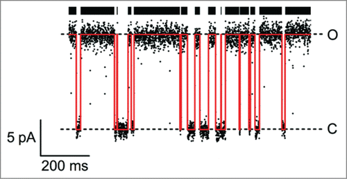
Figure 1. Example of a single-channel trace of a viral Kcv_NTS channel in a DPhPC bilayer in 100 mM KCl at +160 mV (For experimental procedures, see ref. 109). Open-channel current level (O) and baseline (C) are clearly separated. The noise-free time series reconstructed by a Hinkley detector⁵⁴ is drawn in red. The thick black bar symbolizes open events recognized by the detector.

For the first line of analysis, i.e. the determination of the single-channel conductance and the kinetic parameters, this distinction is irrelevant: binding and release constants of a pore blocker can be analyzed with the same algorithms as the opening and closing rates of a spontaneously gating channel. Thus, I shall use the terms fluctuations or flickering which apply to both phenomena, gating or blocking.

The second, more complex step in the analysis is the question of whether observed current fluctuations are caused by intrinsic conformational changes of the protein, allosteric effects by agonists or antagonists, by direct blocking of the pore or another mechanism. The distinction can be made by varying the experimental conditions. The methods must be tailored specifically to the problem at hand, only a few shall be named here. For example, Kv channels have an intrinsic voltage-dependent gating; they maintain their rectifying properties even when all possible blockers and ligands have been removed from the buffer.²⁷ In contrast, the so-called inward rectifying K⁺ channels (Kir) are not intrinsically rectifying. Instead, they are blocked at positive membrane voltages by intracellular components like polyamines.^26,28 The kinetic parameters of a pore blocker have a different dependence on membrane voltage than those of a ligand binding on the periphery of the channel, where it cannot feel the electric field.²⁹ Mixing different ligands and varying their concentration shows if they are competing for the same binding site.²⁹ Mutagenesis can help to further test hypotheses e.g., by removing or altering suspected voltage sensor domains³⁰ or disrupting binding sites.⁵

As mentioned above, the kinetic properties of ion channels depend on physiological conditions, such as membrane potential, ion concentrations and a variety of extracellular and cytosolic messengers. A good understanding of the underlying processes is also of great medical importance since e.g. modifications of gating are a frequent result of genetic defects in many hereditary diseases.^8,9,31

Milli- and microsecond current fluctuations

Typically, physiologists and pharmacologists are interested in the millisecond current fluctuations (red lines in Fig. 1), as they determine most physiologically relevant processes, e.g., action potentials.¹ Microsecond kinetics, sometimes also called “flickering” (Fig. 2) are more the realm of biophysicists: whereas these fast processes may at first glance not be immediately relevant for physiological function, their analysis provides crucial clues to the understanding of stability and dynamics of ion channels and their interaction with blockers or other molecules.^24,25,32,33 Furthermore, computational approaches like molecular dynamics simulations are becoming increasingly powerful, and it is expected that they will be able to predict gating dynamics (Fig. 1) based on the dynamics of individual chemical interactions or conformational changes in a protein.³⁴ These calculations require enormous computing times to predict long-lasting phenomena in the ms time window (Fig. 1). Consequently, simulations will first be able to predict the very fast processes in the µs range (Fig. 2). Thus, the techniques for resolving very fast current fluctuations from experimental recordings are expected to furnish the first bridges between MD simulations of gating and ion channel physiology. Recent all-atom simulations already reached a total simulation time of several ms and were able to show single events of large-scale movements in a Kv channel.³⁵ Protein kinetics on a smaller scale potentially require less computation time. For example, several events of critical salt-bridges, which are forming and breaking in the inner gate of a viral K⁺ channel, could already be observed during simulation times of tens of nanoseconds.²¹

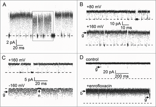
Figure 2. Examples of single-channel traces containing unresolved events. The baseline is marked by a dashed line in each case. (A, B) A human BK channel in an inside-out patch from a HEK293 cell. Currents were filtered at 50 kHz and sampled at 200 kHz. For details on the experimental conditions, see ref. 78. (A) A rare event: The channel switches spontaneously from the dominating gating mode into a fast flickering mode (dotted box) and back. Membrane voltage was +60 mV. (B) The open-channel noise at +80 mV is comparable to the baseline noise. At +160 mV, the open-channel noise is significantly increased (arrow “g”). (C) A viral Kcv_NTS channel in a DPhPC bilayer. Strong flickering is apparent at −160 mV (arrow “g”) as compared to the baseline noise (arrow “n”). Currents were filtered at 1 kHz and sampled at 5 kHz. (Raw data by courtesy of Oliver Rauh, for experimental procedures, see ref. 109.) (D) A porin from E. coli (OmpF) in an asymmetric membrane containing lipopolysaccharides on the trans side, and a mixture of phospholipids and cardiolipin on the cis side. All three pores of the homotrimer have an open probability of nearly 100%; arrows “g” mark closing events of a single monomer. Addition of the antibiotic enrofloxacin causes a flickery block (arrow “b”). Currents were filtered at 5 kHz and sampled at 50 kHz. These traces were previously published in Brauser et al., 2012⁸⁰ in J. Gen. Physiol. doi: 10.1085/jgp.201210776. © A. Brauser. Reproduced by permission of A. Brauser. Permission to reuse must be obtained from the rightsholder.

Brief History of Current Fluctuation Analysis

Revealing single-channel properties

Noise analysis on macroscopic currents

With the reconstitution of purified protein into planar lipid bilayers^36,37 and the introduction of the patch clamp technique^23,38 the quantitative study of single channels became available. Before that, single-channel parameters were only indirectly accessible by extracting them from macroscopic recordings. For very small open probabilities, the variance of the number of open channels follows the Poisson distribution and is equal to the total number N of channels, i.e., ΔN² = N, or given in units of current ΔI² = ΔN²·I_s² = N·I_s² = I_s·I, with I being the macroscopic and I_s the single-channel current (Fig. 1). Since ΔI² and I are macroscopic quantities, I_s can be calculated. For larger open probabilities, the binomial distribution has to be used instead.^7,39 More sophisticated than the analysis of steady-state data is the non-stationary noise analysis, which, depending on the data quality, delivers the single-channel conductance, number of channels and voltage-dependence of the open probability with astounding accuracy.^40,41 The kinetic parameters can be obtained from the corner frequency (−3dB) of the measured noise spectrum.^42-44

Limited resolution of single-channel recordings

The determination of single-channel parameters became much simpler with single-channel recordings by means of the patch clamp technique^23,38 (Fig. 2A, B) and artificial lipid bilayers with recombinant proteins^36,37 (Fig. 2C, D). However, the temporal resolution of single-channel recordings has its limits. Every patch clamp amplifier has a limited bandwidth. The main reason for this is the feedback resistor loop. The first stage of every amplifier is a current-to-voltage converter. Converting a current of 1 pA to at least 1 mV requires a resistor of 1 GΩ, which is shunted by an unavoidable stray capacitance.⁴⁵ The latter limits the speed of the signal response. Thus, it is already impressive that amplifiers with a bandwidth of up to 100 kHz are available. Recently, integrated chip design has enabled bandwidths of up to 1 MHz.⁴⁶

The second limiting factor is the signal-to-noise ratio (SNR). The higher the cut-off frequency of the low-pass filter in the amplifier is set, the higher is the noise amplitude. Recording at 100 kHz filter bandwidth will most likely not be useful, when the SNR falls below 1. Among the critical factors for noise reduction are proper shielding and grounding, a high quality amplifier and low-capacitance patch pipettes. The techniques for noise reduction are reviewed elsewhere.⁴⁷ The SNR of optimized single-channel patch clamp experiments allows a maximum bandwidth of around 30–50 kHz.^32,48 In bilayer experiments, the larger membrane area, and thus, the higher membrane capacitance, cause more noise, further limiting the reasonable bandwidth. The lower access resistance in the open bilayer chamber as compared to a narrow patch electrode partly relieves this problem. The situation can be further improved by optimizing the bilayer capacitance,⁴⁹ but to my knowledge the typical bandwidth of most bilayer experiments is still lower as compared to single-channel patch clamp experiments.

Extending temporal resolution via mathematical analysis

Dwell-time analysis and its limitations

One of the first and still most widespread techniques of single-channel analysis is dwell-time analysis. The number of open or closed events with a duration between T and T+ΔT is plotted versus T.⁵⁰ These dwell-time histograms are fitted with one or more exponentials based on a Markov model. Simple approaches deliver the time constants and the amplitude factors of the exponentials. More sophisticated algorithms deliver the rate constants of the transitions between the assumed states of a Markov model.^51-53

However, the dwell-time analysis has inherent limits in the temporal resolution. The central drawback of dwell-time histograms is the requirement of a jump detector,⁵⁰ which has to assign each measured current value to an open or a closed level (Fig. 1) or to a sublevel. The temporal resolution of these detectors is linked to the filter bandwidth and sampling rate of the recording set-up.⁵⁰ There are several ways to extend the resolution.

Improvements to dwell-time analysis

The standard level detector consists of a band path filter (smoothing out noise, which may lead to “false alarms”) and a threshold detector at a fixed level.⁵⁰ The replacement of this threshold detector by a Hinkley detector (Fig. 1) moderately increased the temporal resolution and enabled the distinction between different sublevels.^54-56 Furthermore, the tape recorder (which at that time was commonly used for data storage) was replaced by a computer hard disk. This increased the sampling frequency to 100 kHz with a bandwidth of 25 kHz. This extension of the bandwidth uncovered that the negative slope conductance in a plant K⁺ channel occurring in the presence of Cs⁺ is not an effect on the single-channel conductance, but instead caused by a fast block.⁵⁷ In the presence of Cs⁺, the current of the open channel is frequently interrupted, which generates an apparent decrease of the open-channel amplitude (Fig. 3B).

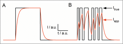
Figure 3. Schematic illustration of the effect of a 1^st order low-pass filter on arbitrary current jumps. (A) A long event (black) and the filtered response (red). (B) The same for a burst of short events. True (I_true) and apparent (I_app) current are indicated by arrows.

The averaging time in the filter of the standard level detector or the integration time in the Hinkley detector had to be a compromise between “false alarms” (fake events caused by spikes from the noise) and “missed events” (events smoothed out by the averaging in the filter). Several groups improved the resolution of dwell-time histograms by applying missed-events corrections.^51,58-61 Farokhi et al. ⁶² demonstrated with simulated data, that after reaching a certain threshold, the time constants of the dwell-time histograms do no longer depend on the value of the rate constants, allowing only limited improvements by missed-events correction after the jump detection.

Hidden Markov model analysis/Direct fit of the timeseries

By sorting single-channel events into one-dimensional dwell time histograms, all information about the sequence of events is lost (but see section 4.4). One way to avoid this is the application of a Maximum-Likelihood predictor to match a Markov model directly to the event sequence. This allows not only to estimate the rate constants of the model but also to choose the best among different candidate model topologies.^63,64 Briefly, the analysis starts with a Markov model with an anticipated set of rate constants (Fig. 5). Based on these rate constants, a one-step algorithm iteratively predicts whether the channel is in a conducting or non-conducting state. From the degree of coincidence of the measured and the predicted current, the Likelihood of the whole time series is calculated. Then, a fitting algorithm suggests a new set of rate constants, and after many iterations, the set of parameters with the highest likelihood is considered the true set of parameters.

Figure 4. Influence of gating on simulated current traces and amplitude histograms from a channel with one open and one closed state, respectively (O-C model, Fig. 5A) in an ideal system without baseline (amplifier) noise (A-E) and with gaussian baseline noise (σ = 1 pA, F-J). The simulated filter was a 4th order Bessel filter with 1 kHz cut-off frequency. The red horizontal lines in the traces indicate the nominal baseline (bottom) and true open-channel current (10 pA, top). Four cases are shown with different rate constants of the transitions between the open and closed states as follows (in s⁻¹): (A, F) k_OC = 200, k_CO = 1 000, black curves in E, J. (B, G) k_OC = 2 000, k_CO = 10 000, red continuous curves in E,J. Resolved and unresolved closing events are marked with arrows labeled “r” and “u,” respectively. (C, H) k_OC = 20 000, k_CO = 100 000, red dashed curves in I,J. (D, I) k_OC = 100 000, k_CO = 100 000, blue curves in E,J. (E, J) Histograms were generated from ca. 300 000 data points, sampled at 10 kHz. Traces in A-I show short representative sections of the same data.

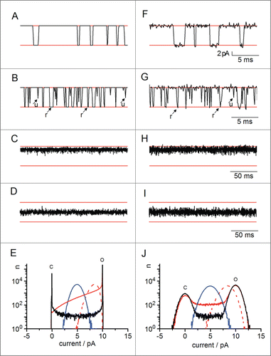
Figure 5. Different Markov models (A, C) and the related (simulated) current traces (B, D) in the case of slow gating in the presence of set-up noise. (A, B) A two-state model. (C, D) A three-state model. Another model with fast flickering inducing increased open-channel noise is shown in Figure 8.

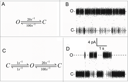
Table 1. Model parameters of the different stages of the beta fit in Figure 8

Panel in Figure 8	Itrue / pA	kFO / s^−1	kOF / s^−1	kOM/s^−1	kMO / s^−1	kSO / s^−1	kOS / s^−1
B, blue	12	300 000	1 000	10	16 000	60	30
B, red	14.65	250 000	64 000	10	16 000	60	30
C, blue	14.65	250 000	64 000	10	16 000	60	70
C, red	14.65	250 000	64 000	588	10 500	60	70
D	14.65	250 000	64 000	588	10 500	60	51
E	14.65	250 000	62 500	660	12 400	97	82

A particular strength of the Maximum-Likelihood predictor is that it can also be applied directly to the raw data of the time series, thus avoiding use of a jump detector (Fig. 1).^65,66 Farokhi et al. ⁶² revealed with this technique rate constants in the range of 50–100 kHz introduced by the Tl⁺-block in the vacuolar K⁺ channel of Chara corallina. Zheng et al.⁴⁸ used another variant of this so-called “Hidden Markov Model analysis” to study the closure of the individual monomers in the Shaker K⁺ channel and found rate constants in a similar temporal range.

However, the problem of level detection is still not completely eliminated as only fully open or closed states are predicted. Many of them are not reached during short dwell-times in the measured time series. Thus, again the missed-events problem came to attention.^60,67,68 The most sophisticated missed-events corrections for Hidden Markov model analysis introduced further sophistications by incorporating the filter of the recording set-up and the noise of the recordings.^69-71

Noise analysis: Spectral analysis

The most efficient approaches of improving temporal resolution do not consider the noise as a nuisance, but as a key. Fast current fluctuations result in small spikes, which cannot be resolved even by the most sophisticated threshold detectors. They appear as “excess noise” which has a higher variance than the baseline noise (noise measured when the channel is absent or closed, Fig. 2).⁷ One approach to utilize this excess noise is the analysis of the frequency spectrum of open-channel noise.⁷² For example, it allowed to exclude shot noise and diffusional processes as the origin of excess open-channel noise in acetylcholine receptors.⁷³ The temperature dependence of the evaluated cut-off frequency suggested fluctuations of the channel protein.

Beta fit Analysis of Fast Current Fluctuations

In my experience, the most powerful approach of extending temporal resolution is the analysis of the amplitude histogram of the measured current trace by means of so-called beta distributions (Fig. 4E).^24,74-77 Similar to the Hidden Markov model analysis, there is no threshold detector required. The idea here is similar to that one mentioned in section Noise analysis on macroscopic currents for the analysis of whole-cell currents, i.e., an analysis of the noise, which is introduced by current fluctuations. The keys to a successful beta distribution analysis are good knowledge of the baseline noise and of the filter step response used during data recording (Fig. 3).

A closer look at the effects of fast current fluctuations on single-channel recordings

Gating (or blocking) events above the bandwidth of the recording setup cause characteristic artifacts in single-channel current records: an increased open-channel noise and a reduction of the measurable single-channel current. Figure 2 presents some examples:

• Human BK channels sometimes exhibit spontaneous mode switching. In the dominant gating mode, the true single-channel current is visible (Fig. 2A, left- and right-hand side). The spontaneous transition to the transient fast gating mode makes the current reduction (Fig. 2A, boxed) immediately apparent.⁷⁶

• At positive membrane potentials of BK, the open-channel noise is much higher (arrow “g” in Fig. 2B) than at negative potentials. This is an indication of current reduction by fast flickering. However, in this case, the true single-channel current is not a priori known as in Fig. 2A and thus has to be determined by the analysis.^32,78

• The viral K⁺ channel Kcv_NTS shows flickering at positive and negative membrane voltages.⁷⁹ At negative voltages, the resulting open-channel noise is extreme (arrow “g” in Fig. 2C), because the unresolved closed events are very frequent and their average duration is only moderately shorter that the response time of the recording apparatus (1 ms).

• Short current interruptions are not only be caused by gating, but also by fast association/dissociation of blockers. For example, this is the case for the antibiotic enrofloxacin, which is blocking the E. coli porin OmpF in the presence of millimolar concentration of Mg²⁺ (Fig. 2D, arrow labeled “b” in bottom trace and ⁸⁰). In blocking experiments, the full current amplitude is usually known from control experiments (Fig. 2D, top) trace. Situations like this one are a good test of the reliability of determining the true current as a fit parameter.

The reason behind both the apparent current reduction of the open-channel amplitude and the increased open-channel noise in the examples in Figure 2 is the distortion of the current trace by the low-pass filter inherent to the recording setup. Figure 3 schematically illustrates the effect of current fluctuations on fictitious noise-free single-channel currents. For the sake of simplicity, a first-order filter is used here. The channel is assumed to open and close instantaneously (Fig. 3, black curve). Only if the length of the open state is longer than the rise time of the pulse response of the filter the recorded current can reach the full value of the current in the open state (Fig. 3A, red curve). Additionally, the length of the event can be properly estimated from the filtered data. However, if the rate constants become faster (Fig. 3B) the dwell-times in the open and closed states are too short, and the measured current during a burst neither reaches the full open channel level nor the baseline (Fig. 3B, red curve). As a result, the experimenter does not record the true level of the open-channel amplitude (Fig. 3, I_true) but an averaged apparent current (Fig. 3, I_app) somewhere between the levels of the C-state and the O-state. Since most channels open in bursts, which are separated by longer closed events, the experimenter will recognize the difference in the noise of the open and the closed level, thus realizing the involvement of fast current fluctuations. As a very clear example, compare the baseline noise at the arrow labeled “n” in Figure 2C with the open-channel noise at the arrow labeled “g.” However, there are exceptions, as for example in bacterial porins with an open probability of close to 100%. In this extreme case the baseline is essentially not visible (see Fig. 2D and section Revealing fast blocking events in OmpF: multi-channel fit with incomplete blocking events, below).

How fast current fluctuations and the noise from the recording set up modify the shape of amplitude histograms

It has already been mentioned that the key for the analysis of fluctuation-induced open-channel noise (Fig. 2) is to interpret the filter artifacts not as a nuisance but as a tool. The low-pass filter distorts the current time series (Fig. 3) as well as the amplitude histograms in a predictable manner, depending on the filter characteristics (type, cut-off frequency, order) and the kinetic properties of the channel. The filter characteristics are known from the manufacturer's information or can be measured. The challenge is to extract the true current and the rate constants from the data.

In an (imaginary) unfiltered, noise-free current trace (black lines in Fig. 3), the current would switch instantaneously, with no data points between the nominal open level and the baseline. The amplitude histogram would consist of 2 infinitely narrow peaks giving the number of sampling points in the open or in the closed state (not shown). In the case of channels with several closed or open states of different dwell-time, the effect of low-pass filtering on current traces and amplitude histograms can be quite complex. An example for measured data is shown below in section Recipe for the fitting of beta distributions. For illustrative purposes, here, the simplest case of a channel gating spontaneously between a single open and closed state (Fig. 5A, below) is demonstrated on simulated data sets. Simulations were done with and without baseline noise.

Filtered, noise-free slow gating generates smooth transitions from the baseline to the full open state and back (Figs. 3A and 4A) causing slight distortions at the edges of the C and O-peaks and a low “bridge” between the 2 peaks (black line in Fig. 4E). In this simulation, both the rate constant of channel opening k_CO = 1 000 s⁻¹ and channel closing k_OC = 200 s⁻¹ are significantly slower than the filter frequency (1 kHz). This is still deep in the realm of dwell-time analysis without missed-events correction; hence the full amplitude and length of the events are clearly visible. The asymmetry of k_OC and k_CO results in a higher population of the open state (compare the height of the black peaks in Fig. 4E).

When the gating rate constants in the simulation are both increased by a factor of 10 (k_OC = 2 000 s⁻¹, k_CO = 10 000 s⁻¹), many of the short channel closings are sufficiently smoothed by the filter so that they do not reach the baseline (arrows “u” in Fig. 4B). In a dwell-time analysis, this would already lead to many missed events. In the noise-free amplitude histogram, the many short closed events, which do not reach the baseline, result in a broad “shoulder” at the O-peak (continuous red curve in Fig. 4E). Because the gating is only moderately fast and some events can still be resolved (arrows “r” in Fig. 4B), this shoulder extends all the way down to the baseline (peak “C” in Fig. 4E)

If the rate constants are further increased by a factor of 10 (k_OC = 20 000 s⁻¹, k_CO = 100 000 s⁻¹), they are so high above the filter frequency (1 kHz) that the gating transitions are no longer obvious (Fig. 4C). Instead, the average current in Figure 4C is reduced. Additionally, the trace appears noisy, even though no noise was added in the simulation. This is caused by the fluctuations in the low-pass filter's jump response to the current jumps as illustrated in Figure 3. In the amplitude histogram, this trace appears as a single peak near the open level (dashed red line in Fig. 4E). The peak position is defined by the open probability p_O = k_CO/(k_OC+k_CO); skewness and width of the peak are defined by the absolute values of the rate constants.

When this kind of fast gating is symmetric (k_OC = k_OC = 100 000 s⁻¹, Fig. 4D), the amplitude histogram shifts into the middle between the O level and the baseline, according to p_O = 0.5; it also becomes symmetric (blue line in Fig. 4E).

In real experiments, baseline noise is superimposed on the current traces (Fig. 4F-I). If the signal-to-noise ratio is large enough, the excess noise caused by fast gating is still visible in the traces. For example, the fast gating traces in Fig. 4H and I are noticeably noisier than the slow gating traces in Fig. 4F and G, even though the same amount of baseline noise was used in the simulation. In the amplitude histograms, the peaks are broadened by a convolution of the amplitude histogram of the gating-induced noise with the Gaussian distribution of the baseline noise. This convolution partially hides the features of the gating-induced excess noise. For example, when set-up noise is added, the asymmetry of the red dashed peak (very fast, asymmetric gating) is diminished in Fig. 4J as compared to Fig. 4E, though still clearly detectable. This phenomenon is the reason why good data quality (low set-up noise) is crucial for a successful analysis using amplitude histograms: if the set-up noise is too large, it will hide the features of the fluctuations-induced excess noise.

The targets of the analysis of fast current fluctuations by beta distributions

Markov models

Channel gating is usually described by so-called Markov models.^58,81 It is assumed that the channel protein has several distinct states (e.g. “O” and “C” in Fig. 5A, C) with well-defined conductivity. Spontaneous fluctuations in the structure of the protein or effects of drugs cause the channel to switch from one state to another (Fig. 5B, D). These transitions between 2 states are of stochastic nature, and the probability of a transition from state I to state J is described by a rate constant k_ij giving the average number of transitions per second. The transition probabilities only depend on the current state and the rate constants and not on the history of the process. The same mathematical framework can be used for any mechanism that stochastically switches the current between defined values. For example for a pore blocking experiment, one would replace the terms “open” and “closed” by “open” and “blocked” and the rate constants would describe the association/dissociation kinetics of the blocker.

Selecting the Markov model for fitting the amplitude histograms

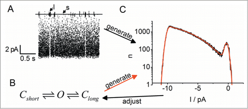
Prior to the analysis of fast flickering, a Markov scheme has to be selected. The number of open and closed states and their arrangement has to be guessed from the current recordings, usually by trial and error. Often, already an inspection of the time series yields clues for the minimum number of states needed to describe the data. The channel used for the example in Figure 6 shows visible (i.e., long) closed events (labeled “l” in Fig. 6A) and short flickery sojourns to a second closed state (labeled “s” in Fig. 6A). This means, at least 2 closed states and one open state have to be employed to describe the gating (Fig. 6B). Starting from the selected model, a theoretical amplitude histogram has to be fitted to the measured one (Fig. 6C). This means that the model parameters have to be obtained by a fitting routine. These parameters are the rate constants, the true single-channel current, and, sometimes also position and noise level of the baseline. The latter step is necessary if the sojourns in the C-level are too short for a reliable direct determination of baseline level and noise. Different methods to generate the theoretical amplitude histograms are discussed in section Generation of beta distributions.

Figure 6. Schematic illustration of the kinetic analysis of amplitude histograms for a channel with one long (arrow “l” in A and state C_long in B), and one short closed state (arrow “s” in A and state C_short in B). The measured current trace (A) and the candidate model (B) are used to create the black amplitude histograms and the red amplitude histogram in (C), respectively. The red theoretical curve has to be generated by one of methods detailed in the text. The model is then adjusted until the theoretical histogram (red) fits the measured one (black). (Raw data by courtesy of Oliver Rauh, for experimental procedures, see ref. 109).

The determination of the “true” single-channel current

The occurrence of fast current fluctuations requires the distinction between “true” (I_true) and “apparent” (I_app) single-channel current. The definition of apparent single-channel current is obvious: it is the value of current, which is obtained from averaging over a section in the current trace of apparently uniform appearance, e.g., over a single burst (e.g., right-hand panel in Fig. 7). Its value can depend strongly on the filter and the length of the selected range of the time series. The information, which can be extracted for biophysical research from this value is low. It only provides a lower limit for possible values of I_true. However, I_app may be of physiological importance as it describes the effective transport rate of the channel.

Figure 7. Determination of the true single-channel current by beta distribution fit of separated open-point histograms. (A) Representative bursts of a single BK channel undergoing mode-switching (same recording as in Fig. 2A, different selection). The baseline and the reconstructed true current (I_true) from the fast mode (right-hand burst) are marked by dashed horizontal lines. The open- and closed-point histograms in the fast gating part were separated by a jump detector. (B) Full (black) and open-point (blue) histograms of the complete fast-gating section of the current trace. Current levels marked as in A. Red shows the beta distribution fit with data simulated from a 2-state model (Fig. 5A) to the open-point histogram. The apparent current in the fast gating mode is approx. 5.7 pA. The fitted true current is with 7.29 pA very close to the current of the slow gating mode serving as a control (7.37 pA). Minor differences to the previous analysis of the same data set⁷⁶ are due to refinements of the method since then.

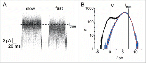
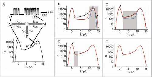
Figure 8. Stages of a beta fit analysis by simulation on the example of a Kcv_S channel in a DPhPC bilayer in 100 mM symmetrical KCl at +140 mV. The cut-off frequency of the 4-pole Bessel filter was 1 kHz. (A) Identification of prominent features in a section of the current trace and the amplitude histogram used to create a candidate Markov model. Markov states are identified with uppercase letters and their identification in the data with arrows and lowercase letters. O: open state; S, s: slow closed state, M, m: medium closed state; F, f: fast closed state. Rate constants between the respective states are defined in the model. (B-E) Comparison of the measured (black) and theoretical data (blue and red) at different stages of the analysis. The rate constants used to generate the theoretical data are shown in Table 1. (B) Before (blue) and after (red) the true single-channel current and the transition O-F have been adjusted to the open peak (shaded area) by changing the current manually and automatically fitting k_FO and k_OF. Special attention is given to the outer flank of the peak (arrow). (C) Before (blue) and after (red) the steepness of the slope (shaded area) has been fitted by manual increase of k_MO. (D) After the slow closed transition O-S has been fitted automatically to match the height of the closed peak (arrow in C and D). Last to be fitted is the shaded area by changing k_OS and k_SO by the same factor. (E) Final result. (Raw by data courtesy of Oliver Rauh, for experimental procedures, see ref. 109.)

The definition of I_true is as follows: in a recording set-up with an infinite bandwidth (i.e, without any filter) a time interval T longer than the interval between the transitions of 2 ions should exist. If the average value of current in an interval shorter than T is independent of the length of the interval, then the current is I_true.⁸² This is a theoretical definition of the true current, but unfortunately not a recipe for its experimental determination.

In real experiments, a more pragmatic definition of I_true has to be used: When the open-channel noise is equal to the baseline noise, we consider this measured current at I_true. However, it has to be kept in mind that undetected fluctuations may be so fast, that it does not increase the open-channel noise. Nevertheless, since there is no better way to detect this, this realistic definition has to be used.

According to the realistic definition of I_true, there are several approaches to its determination:

1. It may occur that the absence of fast current fluctuations is indicated by an open-channel-noise, which is not broader than the baseline noise. Then I_true is equal to I_app. Such a situation is found in the trace of Figure 2A on either side of the flickering section or in Figure 2C at positive potentials. It is also the case in Figure 2D in the absence of enrofloxacin. Especially, situations similar to that in Figure 2D may occur, when traces with and without a drug are compared. This approach enabled several workers to use a well-defined and fixed value of I_true by analyzing amplitude histograms.^24,25,83,84

2. When no control experiments and/or no traces are available with the open-channel noise being equal to the closed-channel (baseline) noise, I_true has to be determined from the analysis of beta distributions. An example for an early investigation extracting the true current by fitting a beta distribution is provided by the analysis of short “interrupts” of 0.3 µs in records of a K⁺ channel in Saccharomyces cerevisae.⁸⁵

The extraction of I_true from the beta fit can be tested either with simulated data or in a situation in which the true single-channel current is already known a priori. The latter case is presented in the following example: BK channels sometimes spontaneously enter a flickering mode and then switch back to their normal behavior⁸⁶ (see also Fig. 2A). Figure 7 shows 2 representative bursts with this phenomenon, both from the same recording. The true current of ca. 7.4 pA can be obtained directly from the recording of the channel in the normal gating mode (burst on the left in Fig. 7A). During the fast flickering mode, the apparent current is significantly reduced (burst on the right in Fig. 7A). Here, I_true has to be determined by beta fit analysis. For this procedure, the bursts of flickering were isolated to generate separate open- and closed-point histograms (Fig. 7B). This trick allows to ignore all longer closed states in the Markov model, which is used for the fit. In this case the open-point histogram of the fast flickering burst (blue in Fig. 7B) can be fitted with a simple 2-state (O-C) model (Fig. 5A).

I_true was included in the set of free fitting parameters in Fig. 7B, together with the 2 rate constants k_CO and k_OC (Fig. 5A). The best fit could be achieved when the true current was set to a value almost identical to the current measured in the non-flickering section. The line marking the fit parameter I_true for the fast gating section (ca. 7.3 pA right-hand side in Fig. 7A) nicely coincides with the current in the slow gating mode (ca. 7.4 pA, left in Fig. 7A). The result of this analysis shows that it is not the open-channel conductance, but a change in channel gating, which is responsible for the lower amplitude during mode-switching of BK. Additionally, the results show, that only the rate of channel closing (k_OC) spontaneously changes by a factor of 4, while the other one remains constant.⁷⁶

Generation of beta distributions

Analytic solution for simple models

For first-order filters and 2-state Markov-models (Fig. 5A), the theoretical amplitude histogram can be calculated analytically. The complete mathematic framework for this technique was formulated initially by FitzHugh⁷⁴ and for the first time applied by Yellen.²⁴ The shape of the amplitude histogram can be described as a beta distribution as given by the following probability density function, f(y):${\displaystyle f\left(y\right)=y^{a-1}(1-y{)}^{b-1}/B\left(a,b\right)}$where the current y is normalized to the interval 0-1. The rate constants are normalized to the filter cut-off frequency f_3db: a = k_CO/f_3dB, b = k_OC/f_3dB. B(a,b), the beta function, is used to normalize the integral over f(y) to 1. ^24,74 For a comparison with the experimental data, f(y) has to be convoluted with the histogram of the baseline noise.

The premise of a 2-state Markov model can be fulfilled in many cases, for example by isolating bursts of fast flickering from the current recordings (Fig. 7B) or by subtracting the baseline distribution directly from the amplitude histogram.²⁴ However, first-order filters are practically never used in patch clamp or bilayer recordings; usually Bessel filters of 4^th and 8^th order are employed.⁵⁰ Sometimes, this problem can be circumvented by introducing a correction factor for the order of the filter, but this works only under a very narrow range of conditions.²⁴

With this technique, it was possible able to resolve the fast Na⁺-block of Ca²⁺-activated K⁺ channels in bovine chromaffin cells; the data show that blocking of the K⁺ channel by Na²⁺ was very voltage-dependent whereas unblocking was voltage-independent.²⁴ In his seminal paper, Yellen explains the extreme voltage dependence of the effect by a diffusion limitation. Driven by voltage, K⁺ passes through the channel extremely quickly, and thus, becomes depleted at the channel mouth (see also section Voltage-induced K⁺ depletion in BK as a cause for fast gating). Unlike K⁺, Na⁺ cannot escape through the channel and does not deplete. With increasing voltage, the relative enrichment of Na⁺ becomes stronger, increasing the chance of Na⁺ to block the channel.

Other typical applications of analytically derived beta distributions include the analysis of the block by Cs⁺,⁸³ and Na^{+ 25} in the dominant tonoplast K⁺ channel of Chara corallina, the cocaine block of purified ryanodine receptors⁸⁴ and the voltage-dependent and Ca²⁺-independent flickering of the outward-rectifying K⁺ channel in Saccharomyces cerevisiae.⁸⁵

An alternative approach, describing the amplitude histograms of channels with rapid kinetics was used by Heinemann and Sigworth.³³ Instead of a beta distribution they used the sum of gaussians and their higher-order cumulants to analyze the ca. 1 µs short closures of gramicidin channels recorded at 10 kHz bandwidth. While this approach is successful in this special case, it is less versatile than beta distributions because the approximations necessary for this method are only valid, if the closed events are rare and much shorter than the filter rise time.

Enhanced analytic methods

As mentioned above, the analytical approach to beta distribution analysis is restricted to 2-state models (Fig. 5A) and first-order filters. However, patch clamp experiments usually use 4th or 8th – order Bessel filters.⁵⁰ In this case, a set of differential equations describes the amplitude histograms. There is no analytic solution for these equations. Their solution and even their constraints have to be obtained from iterative fitting routines.⁸⁷ In addition, the limitation to 2-state models can be overcome by using the theory of extended beta distributions, which allows for aggregated Markov models (Fig. 5C).^77,87 However, again, the resulting differential equation system cannot be solved analytically, but has to be integrated numerically. The most sophisticated analytical method incorporating both multi-state models and higher-order filters (without the use of correction factors) using a Maximum Likelihood approximation was derived by White and Ridout.⁷⁵ To avoid numerical integration, they used a number of simplifying assumptions.

Beta distribution fit based on simulations

By virtue of the increase in computer power since the pioneering work of Yellen²⁴ and FitzHugh,⁷⁴ the problem of generating beta distributions can now be solved by simulations. Based on the assumed Markov model a time series is generated (see Fig. 5 for 2 examples). This generation has to include all features, which are known to have contributed to the generation of the measured time series e.g., the low-pass filter and sampling, but also all kinds of set-up noise. The first requirement is the assumption of an adequate Markov model, and the assignment of distinct current levels to the states of the model. Then, a computer program is required, which provides stochastic numbers that select the sink state of the next transition and the time of this transition in agreement with the values of the (assumed) rate constants of the Markov model. Usually, the rate constants and current levels are not known a-priori and have to be adjusted iteratively during the fitting routine.

In the simulation, it is important to calculate the transition times, i.e. the time points of the jumps between different Markov states, in continuous time, or at least with a much higher temporal precision than the sampling interval in the experiment. Otherwise, the dwell-times could only be multiples of the sampling interval, and especially, they could not be shorter than the sampling interval. This would lead to serious errors when using rate constants faster than the sampling frequency. In the first step, the resulting time series is presented by a list of numbers of the transition times and the related sink states. In the next step, this time series is filtered by a filter with a step response equal to that of the recording set-up. Then, the simulated current trace is sampled.

Noise can be superimposed in 2 different ways. One way is to add the baseline noise directly to the current trace before sampling, and then create the amplitude histogram from this time series. However, since beta fit analysis does not use the current trace, but only the histogram, the amplitude histogram with set-up noise can be obtained by convoluting the histogram of the simulated noise-free, filtered and sampled current trace directly with the (typically Gaussian) distribution of the baseline noise. This saves on computing time.

The distribution of the baseline noise of the measured current trace can be directly determined when closed events of sufficient length are available. If this is not possible, position and width of the baseline noise can also be determined during the analysis. However, one should keep in mind that a larger number of free parameters often lowers the accuracy of the analysis.

The theoretical amplitude histogram is compared with the measured amplitude histogram (Fig. 6C). This step is repeated many times, with the parameters (I_true, the rate constants, and sometimes baseline level and baseline noise) being modified under the guidance of a fitting routine until the measured and the theoretical amplitude histograms coincide.

Basing the construction of the theoretical amplitude histograms on simulations instead of analytical calculation offers a large flexibility. Some features, which can be implemented in a straightforward way, are:

• multi-state Markov models (see section Recipe for the fitting of beta distributions) or even non-Markovian models

• more than one channel (see section Revealing fast blocking events in OmpF: multi-channel fit with incomplete blocking events)

• any kind of filter responses, measured or calculated

• non-gaussian set-up noise, colored noise and periodic perturbations

• adding the set-up noise in the time domain (i.e., to the simulated time series) or convolution of the histogram of the set-up noise and the histogram of the simulated time series. After the calculation of the histogram, all temporal information is lost and only the shape of the noise distribution will influence the fitting process.

One example of noise, which may be considered, is shot noise of the single-channel current. Usually, the single-channel current is treated as a fixed value, which is constant during each channel opening and also does not change between one open event and the next one. However, the movement of ions is stochastic, thus, the number of ions passing the open channel during a given interval is not constant, but varies according to the Poisson distribution: the standard deviation of N ions passing in a given time interval will be √N.⁷³ While this can be relevant for a full description of channel function shot noise can mostly be ignored at now-a-days temporal resolution of channel recordings.⁸⁸

Recipe for the fitting of beta distributions

Fitting can be done with different degrees of complexity. In some experimental data, slow and fast events are well separated. Then, the open-peak of the histogram can be separated from the closed-peak, e.g. by separating sojourns in the C-level and bursts by a jump detector. In this case, a 2-state Markov model is sufficient. This applies for example to the investigations of Yellen²⁴ and to the data from a BK channel described in section Voltage-induced K⁺ depletion in BK as a cause for fast gating (Fig. 7).³² In other time series, slow, medium and fast kinetics are not clearly separated (e.g., Fig. 2C, lower trace). Then, the whole amplitude histogram has to be fitted by a Markov model with more than 2 states.

For Markov models with more than 2 states, an iterative fitting routine, which is switching between automatic fitting and manual interference, has been previously described in detail for the human BK channel, (program “bownhill” available on request).⁸⁹ Here I demonstrate this approach for the spontaneous fast flickering of the viral K⁺ channel Kcv_S in order to show that different channels may require different modifications of the fitting procedure. Kcv_S was expressed in vitro and reconstituted in a DPhPC bilayer in 100 M KCl on either side of the membrane. In the time series used for the amplitude histogram in Figure 8, the current was recorded at +140 mV for 60 s with a 1 kHz 4-pole Bessel filter and a sampling frequency of 5 kHz. For a reliable analysis, it is important, that the current trace is free from drift and other artifacts.

The analysis starts with the selection of an adequate Markov model (Fig. 8A, middle). If no a-priori knowledge is available (e.g., from the analysis of previous experiments) a first guess can be made from the characteristics of the current trace and the amplitude histogram (Fig. 8 top and bottom, respectively). One long closed state is needed for the visible long closed events in the current trace. They are represented in the histogram by the Gaussian shaped closed peak (state “S” = slow and arrows labeled “s” in Fig. 8A). The existence of a second, medium length closed state M is indicated by short closed events that are still visible in the trace, but already considerably attenuated by the filter (arrow labeled “m” in Fig. 8A). The gating speed of these events is moderately above the filter frequency. The transitions between the open state and M cause the long slope between the O and C peaks in the histogram (arrow labeled “m” in Fig. 8A). The third, even shorter closed state (“F” = fast) is visible as a slight increase in the open-channel noise in the trace. In the histogram, this corresponds to broadening of the tip of the O-peak in comparison to the C peak (arrow labeled “f” in Fig. 8A). The existence of more states cannot be excluded. These states are included in so-called reserve factors which cannot be avoided in any kind of kinetic analysis.⁹⁰

Regarding the topology of the Markov model, it is important to mention that different models with the same number of states, but different interactions can produce identical amplitude histograms. The reason is the loss of the temporal order of events during the construction of the histogram from the simulated or measured current records. Thus, unless there is no additional information dictating the model topology (e.g., by using 2-dimensional dwell-time analysis^91,92), we are free to select a convenient one. In the case of channels with a single open state, it is most convenient to use a model with all closed states being directly connected to the open state (“star-shaped,” Fig. 8A), since the inter-dependency between the fit parameters (rate constants) is minimized. If future analysis will show that a different model is more adequate, the rate constants of one model can be mathematically transformed into those of the other model.⁹³ According to these considerations, the star-shaped Markov model of Fig. 8A is used for simulating the theoretical data.

A four state model, which is adequate for Kcv_S, has 7 to 9 free parameters. These are the 6 rate constants (Fig. 8A) and the true single-channel current I_true. In the present case, the position and noise of the baseline can be sufficiently well determined from slow closed events (label “s” in Fig. 8A), so that they need not to be included into the set of free fitting parameters. Experience shows that automatic fitting routines often get stuck in local error minima when trying to adjust all parameters at once. Instead, a mixture of automatic fitting and manual interference is required.

A set of starting values for the model parameters is used to generate the first guess for the theoretical amplitude histogram (Table 1, first row). These values may be arbitrary or obtained from the knowledge from previous fitting routines. During the fitting routine, which is detailed below, each one of the parameters can either be held fixed, modified manually or set “free” i.e. adjusted by the automatic fitting routine.

Figure 8 illustrates a fitting procedure, which has turned out to be successful in many cases. A rough assignment of the influence of the different transitions between the Markov states to the features of the current trace and the amplitude histogram is given in Figure 8A for reference.

Step 1: The fit starts from the following set of parameters, generating the blue curve in Figure 8B: I_true is taken from the open peak of the amplitude histogram. The rate constant k_F0 = 300 000 s⁻¹ (Fig. 8A) is set to a value typical for fast gating in the Kcv family.⁹⁴ k_MO causing the short gaps has to be higher than the filter frequency, e.g. 16 000 s⁻¹. The reverse rate constants k_OF and k_OM are set to small values in order to suppress the effects of these gating processes in this first run. The ratio of the slow rate constants k_SO and k_OS determines the ratio of data points assigned to the C-peak and to the O peak. The lengths of the closed times and burst durations makes k_OS = 30 s⁻¹ and k_SO = 60 s⁻¹ a reasonable suggestion.

The mismatch of the theoretical blue curve and measured amplitude histogram (black) in Figure 8B leads to the following conclusions: The O-peak of the measured data is much broader than that of the simulated one which here is still determined by the baseline noise (shaded area in Fig. 8B). This implies a strong contribution of fast gating (state F in Fig. 8A). The difference between the measured black slope between the O-peak and the C-peak and the calculated horizontal area of the blue curve (Fig. 8B) indicates the involvement of medium gating (state M in Fig. 8A).

Step 2: The O-peak (shaded area) is fitted first by an automatic fit of k_FO and k_OF. This fit has to be repeated for several values of I_true until a reasonable fit of the O-peak is obtained (Fig. 8B, red curve).

Step 3: The red O-peak in Figure 8B is still too high. This can be attenuated by changing k_OS, preferable by stepwise manual adjustments (blue curve in Fig. 8C).

Step 4: Now, k_OM and k_MO are adjusted in order to fix the gap between the blue fit curve and the measured data at the slope between the O-peak and the C-peak (shaded area in Fig. 8C). k_MO determines the inclination of the slope, k_OM its parallel shift (Fig. 8A). The result is the red curve in Fig. 8C. These simple assignments often make a manual adjustment of these rate constants more efficient than an automatic fit. The filling of the gap under the slope influences the distribution of data points between the O-peak and the C-peak (arrow in Fig. 8C). This leads to the next step.

Step 5 : The ratio k_OS/k_SO has to be readjusted to correct the heights of the peaks (arrow in Fig. 8D).

Step 6: The gap between the red and black curve in Fig. 8D (shaded area) at the minimum of the slope can be closed by increasing k_OS and k_SO by the same factor, thus not disturbing the balance of the peaks. In addition, minor adjustments of all other rate constants lead to the final fit shown in Figure 8E.

Depending on the shape of the amplitude histogram, modifications of the above procedure may be required. In lucky cases automatic fitting with 4 free parameters (k_OF, k_FO, k_OM, k_MO, Fig. 8A) is successful. Then, only k_OS and k_SO have to be adjusted in order to provide the correct heights to the peaks and to close the gap at the minimum of the slope (as in Fig. 8D, E). In other cases, slope and O-peak are merged. Then, the skewness of the O-peak (arrow “f” in Fig. 8A) is hidden. In this situation, the exact determination of I_true and the fast rate constants k_FO and k_OF can become impossible. Nevertheless, it is still possible to extract interesting information from these distributions such as the lower and upper limit of these parameters. The respective information can be obtained from the outer flank of the histogram, which is still broader than the baseline (arrow in Fig. 8B).

Additionally, it has to be mentioned, that the shortest closed state F is near the resolution limit of the beta fit, since its decay rate constant k_FO is more than 200 fold above the filter cut-off frequency. In the case that this value were any faster, the excess noise caused by it would no longer be detectable and thus, inaccessible to the analysis.

Examples for Analysis of Fast Current Fluctuations by Beta Distributions

Voltage-induced K⁺ depletion in BK as a cause for fast gating

A prominent example for the effect of fast gating is the occurrence of a negative slope in single-channel IV curves. This kind of negative slopes was recorded from hBK channels heterologously expressed in HEK293 cells (Figs. 2B and 9A and ref. 32). Without further analysis, it could be assumed that the open-channel current saturates or even decreases at extreme positive potentials. However, a closer inspection shows the increase in open-channel noise at positive voltages (Fig. 2B). This indicates that the reduction of the single-channel current with positive voltages is not a real reduction of the conductance, but a result of fast current fluctuations. Knowing the correct single-channel current is essential e.g., when modeling IV curves.^95-97

In order to keep the analysis simple, the bursts of fast flickering were separated from the baseline by means of a level-detector (Fig. 6B). Thus, the open-point amplitude histograms could be analyzed with a 2-state model delivering I_true, k_CO and k_OC (Fig. 5A). The true IV curve (Fig. 9A) does not contain a negative slope; it saturates at high positive voltages. The rate constants of BK flickering are very high (Fig. 9C), and extend to times below 1 µs⁻¹. In this situation, the beta distributions become very narrow and very close to the Gaussian baseline noise. The skewness of the open-point histogram in Fig. 9B is quite weak. Thus, the estimation of the baseline noise has to be very accurate. According to this problem, the errors in the estimation of the absolute values of the rate constants are large (error bars in Fig. 9C). Nevertheless, it is obvious that k_OC is clearly voltage-dependent, whereas k_CO is quite constant (Fig. 9C). In contrast to the absolute values of the rate constants, we have found that the ratio of the opening and closing rate constants is highly reproducible. Fortunately, it is this ratio, which determines the difference between I_true and I_app. The ratio I_true/I_app = (k_OC+k_CO)/k_CO has a simple exponential dependence on membrane voltage (Fig. 9D).³²

Figure 9. Voltage-dependent fast flickering in excised patches of HEK293 cells transfected with the human BK α and β1 subunit in symmetric 150 mM KCl + 2.5 mM CaCl₂ + 2.5 mM MgCl₂ + 10 mM HEPES, pH 7.2. (Schroeder & Hansen, 2007.³² Data originally published in J. Gen. Physiol. doi: 10.1085/jgp.200709802. © I. Schroeder. Reproduced by permission of I. Schroeder. Permission to reuse must be obtained from the rightsholder.) Data in A, C and D are shown as mean and standard deviation (for the number of experiments in each case, see ³²). (A) Apparent single-channel IV curve in BK channels displaying a negative slope at positive potentials (closed squares) and the reconstructed IV curve of I_true (open squares). (B) Representative amplitude histogram of a current trace recorded at +160 mV (black). The open-point histogram is drawn in blue. Red: Fitted amplitude histogram based on the best fit with an O-C Markov model with the true current assumed as indicated in the figure. (C) Rate constants of channel opening (k_CO) and closing (k_OC) resulting from 2-state fits of the isolated open-point histogram as shown in B. For the sake of comparison, the filter cut-off frequency and the approximate rate of ion passage are given by dashed horizontal lines. Experimental conditions as in A. (D) Voltage- and concentration dependence of the ratio I_true / I_app = 1 + k_OC / k_CO in 400 (blue triangles), 150 (red circles) and 50 mM (black squares) KCl with other buffer contents as in A. Continuous lines are single exponential fits.

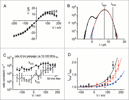
The exponential increase of the gating factor I_true/I_app = (k_OC+k_CO)/k_CO and especially its dependence on K⁺ concentration (Fig. 9D) has led to a hypothesis, which allows to relate function to structure. Based on a simplified model of the channel we can assume that at high positive voltages the ions are pulled out of the selectivity filter to the external side faster than they can enter from the cytosol. Consequently, the effective K⁺ concentration in the pore drops. Since the interaction between K⁺ ions and the carbonyl oxygens of the filter contributes to the stability of the protein,⁹⁸ K⁺ depletion leads to an increase in the rate constant k_OC of channel closure (Fig. 9C). The model proposed by Schroeder and Hansen³² implies that the effect of depletion on gating depends on the average ion concentration resulting from many open-closed events.

The postulated destabilization of the selectivity filter by ion depletion has indeed been documented by many studies, e.g. X-ray crystallography,⁹⁸ energy minimization studies,⁹⁹ MD simulations¹⁰⁰ and tetramerization experiments.^101,102 An early hint to the interaction between selectivity filter and K⁺ ion was the very slow exit rate of a lonely ion, when the repulsive forces of other ions do not help to overcome the binding to the pore wall.¹⁰³ Theoretical studies^99,100 suggest that the selectivity filter, especially the carbonyl group in the second binding site (S2 site) changes its orientation during ion depletion.

The beta distribution analysis also revealed another detail of the BK channel: is has been documented that a block of the channel by cytosolic Ca²⁺ reduces the current of this channel at positive potentials.¹⁰⁴ Analysis of the gating in the absence and presence of Ca²⁺ showed that 2 effects contribute to the current reduction. Without Ca²⁺, the calculated I_true results in a linear IV curve. Ca²⁺ bends it down to a saturating curve (similar to I_true in Fig. 9A). In addition, the fast gating further bends it down and generates the negative slope. With and without Ca²⁺, the flickery current reduction is of the same magnitude.⁷⁸ This indicates that 2 effects are responsible for the negative slope found in BK at high potentials.

As mentioned above, the rate constants of BK flickering at high positive voltages of ca. 1 µs⁻¹ are near the resolution limit of the beta fit even with a 50 kHz low-pass filter. At a single-channel current of 16 pA, 10⁸ ions pass the channel per second. In other words: one ion is on average passing the channel every 10 ns, or 100 ions during an average 1 µs-long channel opening. If the channel openings were even shorter it would be impossible to distinguish between conductivity and gating from the current records. What we now call a closed event could occur from a brief closing of the channel but it may also reflect the shot noise modulating the distance between the ion transitions.

Ion Depletion-Induced Gating is Also Found in a Viral K⁺ Channel

Kcv channels, which were already mentioned above, are a group of K⁺-selective ion channels from large double-stranded DNA viruses found in fresh and seawater.^105-108 Their structure is that of an extremely reduced Kir channel: 2 transmembrane helices per monomer are connected by a short loop containing the consensus K⁺ selectivity filter sequence and the characteristic pore helix. The protein does not contain any cytosolic or extracellular domains and it is fully embedded in the lipid bilayer.¹⁰⁹ As in other K⁺ channels 4 monomers form the functional homotetramer.

Even though Kcv channels have a very simple design, they still gate spontaneously with surprising complexity. The obvious gating process of Kcv_PBCV-1 is in the ms-range and is barely influenced by membrane voltage.⁹⁴ At higher positive membrane voltages, the open events become noisy (Fig. 10A) and the IV curve sublinear and even exhibits a negative slope (Fig. 10B). This indicates current reduction at extreme voltages by a second, much faster gating mechanism. Analysis of these data with the beta fit revealed strong similarities to the BK channel data so that also in this case ion depletion was the presumed origin of the negative slope at positive potentials.⁹⁴

Figure 10. Voltage-dependent fast flickering in the viral K⁺ channel Kcv_PBCV-1 expressed in Xenopus oocytes measured in the cell-attached configuration with 100 mM KCl, 1.8 mM CaCl₂, 1 mM MgCl₂, 10 mM HEPES, pH 7.4 in the pipette (Abenavoli et al., 2009.⁹⁴ Data originally published in J. Gen. Physiol. doi: 10.1085/jgp.200910266. © A. Abenavoli. Reproduced by permission of A. Abenavoli. Permission to reuse must be obtained from the rightsholder.). Data in B and D are shown as mean and standard deviation (for the number of experiments, see ref. 94). (A) Representative single-channel bursts at various membrane voltages. Note the increased open-channel noise and the apparent current decrease at high positive voltages. (B) Apparent (closed squares) and true (open squares) single-channel IV curve. (C) Fit of a representative data set at +80 mV with a 2-state O-C model (Fig. 5A). Black: closed-point histogram, blue: open-point histogram, red: fit by simulated beta distribution. The apparent single-channel current (I_app, peak of the O distribution) and the true current determined by the fit (I_true) are indicated. Minor differences to the previously published fit⁹⁴ result from an improved fitting routine. (D) The comparison of the gating factors I_true/I_app = (k_OC+k_CO)/k_CO determined for Kcv_PBCV-1 (black open squares) and BK in 400 (blue triangles), 150 (red circles) and 50 mM (black squares) KCl (for details, see Fig. 9) indicate that the selectivity filter of Kcv_PBCV-1 is less stable than that of BK. Continuous lines are single exponential fits.

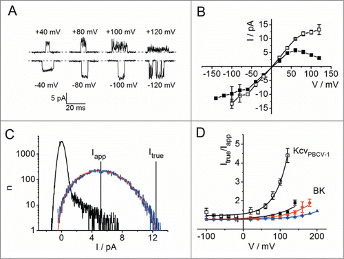
With a more detailed view, some differences to BK are apparent: in the linear range of the IV curves conductance of I_true was higher than that of I_app (Fig. 10B), while the 2 currents coincide in this range for BK (Fig. 9A). Furthermore, the voltage dependence of Kcv_PBCV-1 flickering is about twice as large as in BK, leading to a much larger current reduction (Fig. 10D). Perhaps, the minimal size of the Kcv channel results in a lower stability of the selectivity filter as compared to the larger BK channels.

Revealing fast blocking events in OmpF: multi-channel fit with incomplete blocking events

The analysis with beta distributions is not restricted to ion channels. Bacterial porins are found in the outer membrane of gram-negative bacteria. In its natural form, the protein OmpF from E. coli forms homotrimers of 16-standed β barrels and each monomer is a functional pore.¹¹⁰ These pores are fairly unspecific, anions, cations and small molecules up to 600 Da can pass.^111,112 When the protein is reconstituted in planar lipid bilayers, the ions of the experimental solution (here mainly K⁺ and Cl⁻) cause a quite large conductance that can be easily observed (Fig. 11A).⁸⁰ The open probability of the 3 individual pores is nearly 100% as can be seen from the infrequent closing events (arrows in Fig. 11A, B). None of them reaches the baseline at 0 pA, because in this trace, never all 3 pores close simultaneously.

Figure 11. Analysis of the fast block by enrofloxacin in OmpF (Brauser et al., 2012.⁸⁰ Data originally published in J. Gen. Phys. doi: 10.1085/jgp.201210776. © A. Brauser. Reproduced by permission of A. Brauser. Permission to reuse must be obtained from the rightsholder.). Currents were recorded in an asymmetrical membrane containing lipopolysaccharides on the trans side, and a mixture of phospholipids and cardiolipin on the cis side in 100 mM mM KCl, 5 mM MgCl₂, 5 mM HEPES, pH 7.0 at a bandwidth of 5 kHz. (A) Control experiment. The open probability of all 3 monomeric pores is almost 100%. A few singular (arrows “s”) and double closings (arrow “d”) are visible; the baseline at 0 pA is never reached. (B) In the presence of 0.1 mM enrofloxacin, the current is significantly reduced and the open-channel noise increased. The arrow again marks a closing event. (C) Amplitude histogram of a recording at +100 mV with 0.3 mM enrofloxacin (black), fitted with 3 identical channels with one open and one blocked state, each. Drawn in blue is the best fit result under the assumption that the pore is fully blocked by enrofloxacin. Note the related bad fit at the arrow. Red curve: Best fit result under the assumption that a pore occupied by enrofloxacin still allows a residual current. The fitted residual current is approx. 1/3 of the amplitude in the open state.⁸⁰

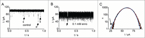
For an antibacterial molecule to reach the bacterium, it first needs to pass the outer membrane. For hydrophilic antibiotics like enrofloxacin, which is commonly used in veterinary medicine, this means, that it needs to pass the porins.^113,114 This makes the interaction between antibiotics and porins an important factor in drug efficacy. Fortunately, passage of larger molecules can be directly observed, because these events briefly block the ionic current. From the kinetic parameters of the blocking events, the “antibiotic conductance” can be calculated.¹¹⁵ However, we found that with Mg²⁺ concentrations near the physiological range, the blocking events become too fast to be resolved directly (Fig. 11B).⁸⁰ The traces show the typical current reduction and increased open-channel noise.

The new challenge for beta distribution analysis was the involvement of 3 parallel channels and incomplete closure by the antibiotic. The analysis was carried out with 3 channels with a simple O-C model for each of the channel pores, which were assumed to be identical. Surprisingly, it was not possible to fit the amplitude histograms under the assumption that the single-pore current switched between fully open (I_true) and fully closed (I_min = 0) as in the case of ion channels.^78,94,116 The best fit was obtained when blocking was assumed to switch between I_min = 0.3 I_true and I_true.⁸⁰ This demonstrates that with sufficient data quality the lower level of the block (or channel closing) can be estimated from the fit in the same way as the true open-channel current.

The results from the beta distribution analysis of OmpF blocking are in good agreement with MD simulations, which showed that only ca. 70% of the diameter of the permeation pathway is blocked.¹¹⁷ Incomplete closure by blocking agents has also been found in other studies employing beta distribution analysis: The inward rectifying substates of human BK channels induced by the toxins BPTI and DTX are actually caused by fast gating between the open state and a very low conductance state.¹¹⁸

Supplementing 2-dimensional dwell-time analysis by the analysis of fluctuation-induced noise

Above it was mentioned that dwell-time analysis is restricted to directly observable events. However, there are strongholds of dwell-time analysis, which make an extension of the temporal range desirable. Two-dimensional dwell-time analysis,⁹¹ which accounts for temporal correlations between transitions of different states, enables the distinction between different Markov models. Huth et al. ¹¹⁹ combined 2D-dwell-time analysis with beta distribution analysis to reveal the sequence of states during the activation and inactivation of Nav1 channels and to determine I_true and the fast rate constants which would be inaccessible in a standard 2D-dwell-time analysis.

The slow rate constants could be taken directly from the dwell-time fit results. In order to determine also the rate constants of the fast transitions, a global fit of dwell-time analysis and beta fit analysis was employed. The analysis started from an assumed value of I_true and the rate constants. From these parameters, a timeseries was generated and used for the construction of the theoretical 2D-dwell-time histogram. A fitting routine (in this case a genetic algorithm¹²⁰) changed the rate constants until the measured and theoretical histograms coincided. In a next step, an amplitude histogram was created from the fit parameters and compared with that of the measured amplitude histogram. Of course, in the first run the 2 histograms would not coincide. Then, the whole procedure from the generation of the theoretical timeseries, fit of the 2D-dwell-time histogram and generation of the amplitude histogram was repeated for different values of I_true, until theoretical and measured amplitude histograms coincided. It may be surprising that the correct estimation of I_true also leads to a reliable determination of the fast rate constants, which would not be accessible from a pure 2D-dwell-time analysis. The robustness of this approach has been tested with simulated data.⁹² The key is to use simulated time series for the fit of the 2D-dwell-time histograms. The simulation automatically takes care of the effects of noise and filter such as missed events and false alarms.

Overcoming the temporal restrictions of bilayer experiments by beta distribution analysis, thus opening the way to “Channel Lego”

A common method for uncovering structure/function correlates in ion channels is the employment of site directed mutagenesis. One important functional parameter under scrutiny is the characteristic gating of a channel. A major problem is to identify those key residues, which are responsible for a certain gating feature. For these studies, the aforementioned large family of viral Kcv channels (K⁺ channel from chlorella virus) offers unique advantages. It has already been mentioned that Kcv channels are small. They range in size from only 79 to 120 amino acids per monomer. Each monomer is made of 2 transmembrane domains, which are connected by the pore helices. ^105-108 A further advantage of these channels is that members differ only by a few amino acids, but show quite different functional properties. This guides the experimenter to those residues, which are crucial for function. Especially, one type of channel behavior can be converted to another by stepwise point mutation. This strategy reveals those residues, which are essential for the individual functional characteristics. Furthermore, chimeras can be created in which 2 of the channels can be swapped. This building of new channels from parts of different origin may be called “channel Lego.”

For the kinetic analysis of these channels, the recording of the electrophysiological parameters from bilayers³⁶ provides important advantages over experiments in living cells. First, even though Kcv channels express in different cell types, currents cannot always be observed.¹²¹ Second, in bilayers there is no interference from the intrinsic channels of living cells. Third, the reproducibility of the records is not decreased by the interference from membrane irregularities, cell cycle, post-translational modifications, etc. Fourth, cell-free expression of membrane proteins has become very powerful by the advent of lipid nanodiscs.¹²² These consist of a protein or polymer scaffold surrounding a lipid double layer with only a few nm in diameter. Among many custom-tailored approaches, now also some commercial systems are available. Especially small membrane proteins spontaneously fold correctly into the nanodiscs and retain their native function.^109,123 Another benefit of cell-free expression is the avoidance of interference from the expression system, e.g., yeast cells or E. coli. Purification of recombinant channel proteins often introduces contaminations like endogenous channels from the expression systems.¹²⁴

The drawback of bilayer experiments is the high electrical capacity of the membrane, which results from the large diameter of the membrane of typically 50–100 µm. Even though the access resistance in a typical bilayer chamber is very low, the high capacitance leads to higher noise as compared to single-channel patch clamp experiments. For example, a typical bilayer experiment in our lab has a noise rms of 0.5 pA at a bandwidth of 1 kHz (unpublished data), whereas single-channel patch clamp experiments reach 1.5 pA noise at a much higher bandwidth of 20 kHz.⁷⁸ This has the consequence that the filter for the bilayer has to be set to values around 1–2 kHz in order to achieve an acceptable signal-to-noise ratio. Thus, some interesting properties in the time series of single-channel traces are not detected by the low temporal resolution of traditional approaches like dwell-time analysis.

The traces in Figure 12A show time series of 2 very similar viral channels¹²⁵ measured in a DPhPC bilayer at +160 mV with 100 mM KCl on either side of the membrane. The apparent single-channel current is very similar (12.7 pA for Kcv_NTS and 13 pA for Kcv_S in the example in Fig. 12). Regarding to their slow gating, the 2 channels are obviously different; the open probability of Kcv_S is considerably lower as that of Kcv_NTS (Fig. 12A). The related gating kinetics are in the millisecond range and even at a filter frequency of 1 kHz well accessible to dwell-time analysis.¹⁰⁹

Figure 12. Beta distributions of Kcv channels. (A) Representative sections of current traces from Kcv_NTS (top) and Kcv_S (bottom) measured in a DPhPC bilayer at +160 mV with 100 mM KCl, 10 mM HEPES, pH 7 on either side of the membrane. (B) Comparison of representative amplitude histograms of longer traces under the same conditions. Black: Kcv_NTS, red: Kcv_S. Currents have been scaled to 0 (C, baseline) and 1 (O, apparent current). Furthermore, the histogram of Kcv_S has been slightly scaled up to match the height of the O peaks. (C) The histograms from a single representative experiment from Kcv_NTS and Kcv_S were fitted with the 5-state model of Fig. 8A. The graph shows the opening (k_MO) and closing (k_OM) rate constants related to the medium closed state M (Fig. 8A) for positive voltages for Kcv_NTS (black) and Kcv_S (red). (Raw data by courtesy of Oliver Rauh, for experimental procedures, see ref. 109.)

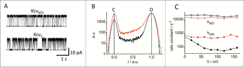
The data show an exemplary case in which beta analysis can reveal kinetic features in numerical terms, which are not immediately obvious from an inspection of the time series. The flickery gating seems to be somewhat more active in Kcv_S than in Kcv_NTS (Fig. 12A). However, the transitions are in both cases just small spikes, which are not suitable for dwell-time analysis. An evaluation of the related amplitude histograms (Fig. 12B) from recordings at different membrane potentials however reveals a distinct difference in the gating of the 2 channels between state O and state M of the model in Figure 8A. The rate constant of opening k_MO is very similar in both channels and hardly effected by voltage (Fig. 12C). The beta distribution analysis however uncovers a significant difference in k_OM (transitions into the closed state M) between the 2 channels at all positive membrane potentials. This striking difference in open-state stability between the 2 channels would most likely have been missed without the analysis of the amplitude histograms.

Summary of experimental prerequisites

The determination of a pair of rate constants (opening and closing reaction) needs 2 prerequisites; the excess noise has to make the amplitude histogram broader than that of the baseline noise and the skewness of the distribution has to be detectable. Three parameters (I_true, k_on and k_off) have to be detected from I_app, the width and the skewness. The major problem is the skewness. If it cannot be detected, there are only 2 measured parameters to determine 3 theoretical parameters. The skewness can be hidden by the baseline noise or just be absent if k_on = k_off. Another possibility is that the current fluctuations are so much faster than the cut-off frequency of the low-pass filter that the filtered excess noise is symmetric. Theoretically, also shot noise may interfere with the analysis. However, we⁸⁸ have shown that at the present state-amplifiers, shot noise can be mostly ignored. The shape of the histogram and thus the performance of the beta fit analysis depends on a number of conditions, both experimental and concerning the channel to be examined:

• –The baseline of the recording must be absolutely stable. Drift or membrane instabilities will otherwise distort the amplitude histograms.

• –The gain during the recording must be high enough. As a rule of thumb, the standard deviation of the noise peak in the amplitude histogram should be at least 10 bins wide, otherwise the shape of the histogram will not be smooth enough to be fitted accurately.

• –For the same reason, the current traces should not be too short. The number of data points has to be high enough to reduce the scatter of the histogram, which has to be much smaller than the difference between the histogram of the baseline noise and that one of the open state.

• –The signal-to-noise ratio should be at least 4:1. Otherwise, the excess noise will be mostly obscured by the baseline noise.

• –Single-channel recordings are preferred over multichannel recordings.

• –The analysis of recordings with not too many states is more reliable because less parameters have to be determined. In my experience, even under ideal circumstances, the amplitude histograms do not provide enough information to fit models with more than 4 or 5 states or 8–10 rate constants.

• –Preferably, the states of the channels are kinetically well separated, (rate constants differ by a factor of 10) allowing them to be assigned to specific regions of the amplitude histogram.

An important computational aspect is that the filter step response and noise distribution implemented in the simulation algorithm must match those in the experiment to avoid the introduction of systematic errors in the analysis.

Conclusion

The great challenge in the field of structural biology is to correlate conformational changes in a protein with functional properties. The present review shows that much information on the fast kinetics of ion channels is hidden in the amplitude histograms of single-channel recordings. Using simulated timeseries to generate beta distributions provides an increase of temporal resolution more than 20-fold over conventional data analysis. This provides the true single-channel current and the gating statistics down to or even below the microsecond range in records with low patch capacitance. This is close to the realm of individual ion passages through the channel pore, and it is expected that beta distribution analysis will bridge the gap between the limited temporal resolution of single-channel recordings and the limited length of conformational trajectories predicted from molecular dynamics simulations. In recordings with low bandwidth like those from bilayers, beta distribution analysis seems to become inevitable to reach the sub-millisecond range, which is still of physiological relevance.

Disclosure of Potential Conflicts of Interest

No potential conflicts of interest were disclosed.

Acknowledgments

I am grateful to Oliver Rauh for the permission to use the raw data of Kcv_S and Kcv_NTS, to Anna Moroni for the data of Kcv_PBCV-1 and Annemarie Donoghue, née Brauser for the data of OmpF. Ulf-Peter Hansen and Gerhard Thiel provided helpful discussion.

Funding

The work was funded by DFG grant SCHR 1467/1-1 to I. Schroeder.

References

- Catterall WA. Voltage-gated sodium channels at 60: structure, function and pathophysiology. J Physiol 2012; 590:2577-89; PMID:22473783; http://dx.doi.org/10.1113/jphysiol.2011.224204
- Hodgkin AL, Huxley A. A quantitative description of membrane current and its application to conductance and excitation in nerve. J Physiol 1952; 117:500-44; PMID:12991237; http://dx.doi.org/10.1113/jphysiol.1952.sp004764
- Goodman BE. Channels active in the excitability of nerves and skeletal muscles across the neuromuscular junction: basic function and pathophysiology. Adv Physiol Educ 2008; 32:127-35; PMID:18539851; http://dx.doi.org/10.1152/advan.00091.2007
- Wahl-Schott C, Biel M. HCN channels: structure, cellular regulation and physiological function. Cell Mol Life Sci 2009; 66:470-94; PMID:18953682; http://dx.doi.org/10.1007/s00018-008-8525-0
- Lolicato M, Bucchi A, Arrigoni C, Zucca S, Nardini M, Schroeder I, Simmons K, Aquila M, DiFrancesco D, Bolognesi M, et al. Cyclic dinucleotides bind the C-linker of HCN4 to control channel cAMP responsiveness. Nat Chem Biol 2014; 10:457-62; PMID:24776929; http://dx.doi.org/10.1038/nchembio.1521
- Urrego D, Tomczak AP, Zahed F, Stühmer W, Pardo LA. Potassium channels in cell cycle and cell proliferation. Phil Trans R Soc Lond B 2013; 369:20130094; http://dx.doi.org/10.1098/rstb.2013.0094
- Hille B. Ion channels of excitable membranes. 3rd ed. Sunderland: Sinauer Associates, Inc; 2001.
- Lehmann-Horn F, Jurkat-Rott K. Voltage-gated ion channels and hereditary disease. Physiol Rev 1999; 79:1317-72; PMID:10508236
- Ashcroft FM. From molecule to malady. Nature 2006; 440:440-7; PMID:16554803; http://dx.doi.org/10.1038/nature04707
- Carpenter EP, Beis K, Cameron AD, Iwata S. Overcoming the challenges of membrane protein crystallography. Curr Opin Struct Biol 2008; 18:581-6; PMID:18674618; http://dx.doi.org/10.1016/j.sbi.2008.07.001
- Loll PJ. Membrane proteins, detergents and crystals: what is the state of the art? Acta Cryst 2014; F70:1576-83;
- Doyle DA, Morais-Cabral JH, Pfuetzner RA, Kuo A, Gulbis JM, Cohen SL, Chait BT, MacKinnon R. The structure of the potassium channel: Molecular basis of K+ conduction and selectivity. Science 1998; 280:69-77; http://dx.doi.org/10.1126/science.280.5360.69
- Santos JS, Asmar-Rovira GA, Han GW, Liu W, Syeda R, Cherezov V, Baker KA, Stevens RC, Montal M. Crystal structure of a voltage-gated K+ channel pore module in a closed state in lipid membranes. J Biol Chem 2012; 287:43063-70; PMID:23095758; http://dx.doi.org/10.1074/jbc.M112.415091
- Kuo A, Gulbis JM, Antcliff JF, Rahman T, Lowe ED, Zimmer J, Cuthbertson J, Ashcroft FM, Ezaki T, Doyle DA. Crystal structure of the potassium channel KirBac1.1 in the closed state. Science 2003; 300:1922-6; http://dx.doi.org/10.1126/science.1085028
- Zhang X, Ren W, DeCaen P, Yan C, Tao X, Tang L, Wang J, Hasegawa K, Kumasaka T, He J, et al. Crystal structure of an orthologue of the NaChBac voltage-gated sodium channel. Nature 2012; 486:130-4; PMID:22678295; http://dx.doi.org/10.1038/486323e
- Van der Cruijsen EAW, Nand D, Weingarth M, Prokofyev A, Hornig S, Cukkemane AA, Bonvin AMJJ, Becker S, Hulse RE, Perozo E, et al. Importance of lipid-pore loop interface for potassium channel structure and function. Proc Natl Acad Sci U S A 2013; 110:13008-13; PMID:23882077; http://dx.doi.org/10.1073/pnas.1305563110
- ww.rcsb.org data retrieved on 05/05/15.
- Berman HM, Westbrook J, Feng Z, Gilliland G, Bhat TN, Weissig H, Shindyalov IN, Bourne PE. The protein data bank. Nucleic Acids Res 2000; 28:235-42; PMID:10592235; http://dx.doi.org/10.1093/nar/28.1.235
- Chen X, Aldrich RW. Charge substitution for a deep-pore residue reveals structural dynamics during BK channel gating. J Gen Physiol 2011; 138:137-54; PMID:21746846; http://dx.doi.org/10.1085/jgp.201110632
- Hertel B, Tayefeh S, Kloss T, Hewing J, Gebhardt M, Baumeister D, Moroni A, Thiel G, Kast SM. Salt bridges in the miniature viral channel Kcv are important for function. Eur Biophys J 2010; 39:1057-68; PMID:19390850; http://dx.doi.org/10.1007/s00249-009-0451-z
- Tayefeh S, Kloss T, Thiel G, Hertel B, Moroni A, Kast SM. Molecular dynamics simulation of the cytosolic mouth in Kcv-type potassium channels. Biochemistry 2007; 46:4826-39; PMID:17397187; http://dx.doi.org/10.1021/bi602468r
- Bertaccini EJ, Dickinson R, Trudell JR, Franks NP. Molecular modeling of a tandem two pore domain potassium channel reveals a putative binding site for general anesthetics. ACS Chem Neurosci 2014; 5:1246-52; PMID:25340635; http://dx.doi.org/10.1021/cn500172e
- Neher E, Sakman B. Single-channel currents recorded from membrane of denerved frog muscle fibres. Nature 1976; 260:799-802; PMID:1083489; http://dx.doi.org/10.1038/260799a0
- Yellen G. Ionic permeation and blockade in Ca2+-activated K+ channels of bovine chromaffin cells. J Gen Physiol 1984; 84:157-86; PMID:6092514; http://dx.doi.org/10.1085/jgp.84.2.157
- Weise R, Gradmann D. Effects of Na+ on the predominant K+ channel in the tonoplast of Chara: decrease of conductance by blocks in 100 nanosecond range and induction of oligo- or poly-subconductance gating modes. J Membr Biol 1990; 282:87-93;
- Kurata HT, Cheng WWL, Nichols CG. Polyamine block of inwardly rectifying potassium channels. Methods Mol Biol 2011; 720:113-26; PMID:21318869; http://dx.doi.org/10.1007/978-1-61779-034-8_6
- Zei PC, Aldrich RW. Voltage-dependent gating of single wild-type and S4 mutant KAT1 inward rectifier potassium channels. J Gen Physiol 1998; 112:679-713; PMID:9834140; http://dx.doi.org/10.1085/jgp.112.6.679
- Lopatin AN, Makhina EN, Nichols CG. Potassium channel block by cytoplasmic polyamines as the mechanism of intrinsic rectification. Nature 1994; 372:366-9; PMID:7969496; http://dx.doi.org/10.1038/372366a0
- Chen L, Gu Y, Huang LY. The mechanism of action for the block of NMDA receptor channels by the opioid peptide dynorphin. J Neurosci 1995; 15:4602-11; PMID:7540680
- Shaya D, Kreir M, Robbins RA, Wong S, Hammon J, Brüggemann A, Minor DLJ. Voltage-gated sodium channel (NaV) protein dissection creates a set of functional pore-only proteins. Proc Natl Acad Sci U S A 2011; 108:12313-8; PMID:21746903; http://dx.doi.org/10.1073/pnas.1106811108
- Bernard G, Shevell MI. Channelopathies: a review. Pediatr Neurol 2008; 38:73-85; PMID:18206787; http://dx.doi.org/10.1016/j.pediatrneurol.2007.09.007
- Schroeder I, Hansen U-P. Saturation and microsecond gating of current indicate depletion-induced instability of the MaxiK selectivity filter. J Gen Physiol 2007; 130:83-97; PMID:17591987; http://dx.doi.org/10.1085/jgp.200709802
- Heinemann SH, Sigworth FJ. Open channel noise. VI. Analysis of amplitude histograms to determine rapid kinetic parameters. Biophys J 1991; 60:577-87; PMID:1718467; http://dx.doi.org/10.1016/S0006-3495(91)82087-2
- Sigg D. Modeling ion channels: Past, present, and future. J Gen Physiol 2014; 144:7-26; PMID:24935742; http://dx.doi.org/10.1085/jgp.201311130
- Jensen MO, Jogini V, Borhani DW, Leffler AE, Dror RO, Shaw DE. Mechanism of voltage gating in potassium channels. Science 2012; 336:229-33; http://dx.doi.org/10.1126/science.1216533
- Montal M, Mueller P. Formation of bimolecular membranes from lipid monolayers and a study of their electrical properties. Proc Natl Acad Sci U S A 1972; 69:3561-6; PMID:4509315; http://dx.doi.org/10.1073/pnas.69.12.3561
- Latorre R, Ehrenstein G, Lecar H. Ion transport through excitability-inducing material (EIM) channels in lipid bilayer membranes. J Gen Physiol 1972; 60:72-85; PMID:5042024; http://dx.doi.org/10.1085/jgp.60.1.72
- Hamill OP, Marty A, Neher E, Sakman B, Sigworth FJ. Improved patch-clamp techniques for high-resolution current recording from cells and cell-free membrane patches. Pfluegers Arch 1981; 391:85-100; http://dx.doi.org/10.1007/BF00656997
- Neher E, Stevens CF. Conductance fluctuations and ionic pored in membranes. Ann Rev Biophys 1977; 6:345-81; http://dx.doi.org/10.1146/annurev.bb.06.060177.002021
- Alvarez O, Gonzalez C, Latorre R. Counting channels: a tutorial guide on ion channel fluctuation analysis. Adv Physiol Educ 2002; 26:327-41; PMID:12444005; http://dx.doi.org/10.1152/advan.00006.2002
- Sigworth FJ. The conductance of sodium channels under conditions of reduced current at the node of Ranvier. J Physiol 1980; 307:131-42; PMID:6259331; http://dx.doi.org/10.1113/jphysiol.1980.sp013427
- Kolb HA, Läuger P, Bamberg E. Correlation analysis of electrical noise in lipid bilayer membranes: kinetics of gramicidin A channels. J Membr Biol 1975; 20:133-54; PMID:47397; http://dx.doi.org/10.1007/BF01870632
- Conti F, De Felice L., Wanke E. Potassium and sodium current noise in the membrane of the squid giant axon. J Physiol 1975; 248:45-82; PMID:1151828; http://dx.doi.org/10.1113/jphysiol.1975.sp010962
- Clay JR, DeFelice LJ, DeHaan RL. Current noise parameters derived from voltage noise and impedance in embryonic heart cell aggregates. Biophys J 1979; 28:169-84; PMID:262547; http://dx.doi.org/10.1016/S0006-3495(79)85169-3
- Sigworth FJ. Electronic design of the patch-clamp. In: Sakman B, Neher E, editors. Single-Channel Recording. New York: Plenum Press; 1983. page 3-35.
- Rosenstein JK, Ramakrishnan S, Roseman J, Shepard KL. Single ion channel recordings with CMOS-anchored lipid membranes. Nano Lett 2013; 13:2682-6; PMID:23634707; http://dx.doi.org/10.1021/nl400822r
- Ogden D, Stanfield P. Patch clamp techniques for single channel and whole-cell recording. In: Ogden D, editor. Microelectrode techniques: the Plymouth Workshop handbook. Company of Biologists Limited; 1994. page 53-78; Cambridge, UK.
- Zheng J, Vankataramanan L, Sigworth FJ. Hidden Markov model analysis of intermediate gating steps associated with the pore gate of shaker potassium channels. J Gen Physiol 2001; 118:547-64; PMID:11696611; http://dx.doi.org/10.1085/jgp.118.5.547
- Wonderlin WF, Finkel A, French RJ. Optimizing planar lipid bilayer single-channel recordings for high resolution with rapid voltage steps. Biophys J 1990; 58:289-97; PMID:1698470; http://dx.doi.org/10.1016/S0006-3495(90)82376-6
- Colquhoun D, Sigworth FJ. Fitting and statistical analysis of single-channel records. In: Sakman B, Neher E, editors. Single-Channel Recording. New York: Plenum Press; 1983. page 191-263.
- Qin F, Li L. Model-based fitting of single-channel dwell-time distributions. Biophys J 2004; 87:1657-71; PMID:15345545; http://dx.doi.org/10.1529/biophysj.103.037531
- Kijima S, Kijima H. Statistical analysis of channel current from a membrane patch. I. Some stochastic properties of ion channels or molecular systems in equilibrium. J Theor Biol 1987; 128:423-34; PMID:2451769; http://dx.doi.org/10.1016/S0022-5193(87)80188-1
- Blunck R, Kirst U, Riessner T, Hansen U-P. How powerful is the dwell-time analysis of multi-channel records? J Membr Biol 1998; 165:19-35; PMID:9705979; http://dx.doi.org/10.1007/s002329900417
- Schultze R, Draber S. A nonlinear filter algorithm for the detection of jumps in patch-clamp data. J Membr Biol 1993; 132:41-52; PMID:7681481; http://dx.doi.org/10.1007/BF00233050
- Draber S, Schultze R. Detection of jumps in single-channel data containing subconductance levels. Biophys J 1994; 67:1404-13; PMID:7529580; http://dx.doi.org/10.1016/S0006-3495(94)80614-9
- Hansen U-P, Albertsen A, Moldaenke C, Draber S, Schultze R. Detecting events in signals from sensors: the Hinkley detector is the answer. Sensors Mater 1995; 7:289-300;
- Draber S, Hansen U-P. Fast single-channel measurements resolve the blocking effect of Cs+ on the K+ channel. Biophys J 1994; 67:120-9; PMID:7918979; http://dx.doi.org/10.1016/S0006-3495(94)80461-8
- Ball FG, Rice JA. Stochastic models for ion channels: introduction and bibliography. Math Biosci 1992; 112:189-206; PMID:1283350; http://dx.doi.org/10.1016/0025-5564(92)90023-P
- Blatz AL, Magleby KL. Correcting single channel data for missed events. Biophys J 1986; 49:967-80; PMID:2423151; http://dx.doi.org/10.1016/S0006-3495(86)83725-0
- Colquhoun D, Hatton CJ, Hawkes AG. The quality of maximum likelihood estimates of ion channel rate constants. J Physiol 2003; 547:699-728; PMID:12562901; http://dx.doi.org/10.1113/jphysiol.2002.034165
- Crouzy SC, Sigworth FJ. Yet another approach to the dwell-time omission problem of single-channel analysis. Biophys J 1990; 58:731-43; PMID:1698473; http://dx.doi.org/10.1016/S0006-3495(90)82416-4
- Farokhi A, Keunecke M, Hansen U. The anomalous mole fraction effect in chara: gating at the edge of resolution. J Membr Biol 2000; 79:3072-82;
- Horn R, Vandenberg CA. Statistical properties of single sodium channels. J Gen Physiol 1984; 84:505-34; PMID:6094703; http://dx.doi.org/10.1085/jgp.84.4.505
- Vandenberg CA, Horn R. Inactivation viewed through single sodium channels. J Gen Physiol 1984; 84:535-64; PMID:6094704; http://dx.doi.org/10.1085/jgp.84.4.535
- Fredkin DR, Rice JA. Maximum likelihood estimation and identification from single-channel recordings. Proc R Soc Lond B 1992; 242:125-32; http://dx.doi.org/10.1098/rspb.1992.0094
- Albertsen A, Hansen U-P. Estimation of kinetic rate constants from multi-channel recordings by a direct fit of the time series. Biophys J 1994; 67:1393-403; PMID:7529579; http://dx.doi.org/10.1016/S0006-3495(94)80613-7
- Hawkes AG, Jalali A, Colquhoun D. Asymptotic distributions of apparent open times and shut times in a single channel record allowing for the omission of brief events. Philos Trans Biol Sci 1992; 337:383-404; http://dx.doi.org/10.1098/rstb.1992.0116
- Hawkes AG, Jalali A, Colquhoun D. The distributions of the apparent open times and shut times in a single channel record when brief events cannot be detected. Philos Trans Phys Sci Eng 1990; 332:511-38; http://dx.doi.org/10.1098/rsta.1990.0129
- Venkataramanan L, Sigworth FJ. Applying hidden Markov models to the analysis of single ion channel activity. Biophys J 2002; 82:1930-42; PMID:11916851; http://dx.doi.org/10.1016/S0006-3495(02)75542-2
- Michalek S, Lerche H, Wagner M, Mitrovic N, Schiebe M, Lehmann-Horn F, Timmer J. On identification of Na+ channel gating schemes using moving-average filtered hidden Markov models. Eur Biophys J 1999; 28:605-9; PMID:10541799; http://dx.doi.org/10.1007/s002490050243
- Fredkin DR, Rice JA. Fast evaluation of the likelihood of an HMM: Ion channel currents with filtering and colored noise. IEEE Trans Signal Process 2001; 49:625-33; http://dx.doi.org/10.1109/78.905892
- Heinemann SH, Sigworth FJ. Open channel noise IV. Estimation of rapid kinetics of formamide block in gramicidin A channels. Biophys J 1988; 54:757-64; PMID:2465033; http://dx.doi.org/10.1016/S0006-3495(88)83013-3
- Sigworth FJ. Open channel noise. I. Noise in acetylcholine receptor currents suggests conformational fluctuations. Biophys J 1985; 47:709-20; PMID:2410044; http://dx.doi.org/10.1016/S0006-3495(85)83968-0
- FitzHugh R. Statistical properties of the asymmetric random telegraph signal, with applications to single-channel analysis. Math Biosci 1983; 89:75-89; http://dx.doi.org/10.1016/0025-5564(83)90028-7
- White PJ, Ridout MS. The estimation of rapid rate constants from current-amplitude frequency distributions of single-channel recordings. J Membr Biol 1998; 129:115-29; http://dx.doi.org/10.1007/s002329900319
- Schroeder I, Hansen U-P. Strengths and limits of Beta distributions as a means of reconstructing the true single-channel current in patch clamp time series with fast gating. J Membr Biol 2006; 210:199-212; PMID:16909337; http://dx.doi.org/10.1007/s00232-006-0858-8
- Riessner T, Hansen U-P. Fast switching in patch clamp records as analyzed by an extended theory of multi-state multi-channel beta distributions. In: Abstracts of the 10th International Workshop on Plant Membrane Biology. Regensburg: 1996
- Schroeder I, Thiel G, Hansen U-P. Ca2+ block and flickering both contribute to the negative slope of the IV curve in BK channels. J Gen Physiol 2013; 141:499-505; PMID:23530139; http://dx.doi.org/10.1085/jgp.201210956
- Braun CJ. Structure/function correlates and protein/lipid interaction of the viral potassium channel KcvNTS. 2014; PhD thesis, Technical University of Darmstadt.
- Brauser A, Schroeder I, Gutsmann T, Cosentino C, Moroni A, Hansen U, Winterhalter M. Modulation of enrofloxacin binding in OmpF by Mg2+ as revealed by the analysis of fast flickering single-porin current. J Gen Physiol 2012; 140:69-82; PMID:22689827; http://dx.doi.org/10.1085/jgp.201210776
- Baum LE, Petrie T. Statistical inference for probabilistic functions of finite state Markov models. Ann Math Stat 1966; 6:1554-63; http://dx.doi.org/10.1214/aoms/1177699147
- Hansen U-P, Cakan O, Abshagen-Keunecke M, Farokhi A. Gating models of the anomalous mole-fraction effect of single-channel current in Chara. J Membr Biol 2003; 192:45-63; PMID:12647033; http://dx.doi.org/10.1007/s00232-002-1063-z
- Klieber H-G, Gradmann D. Enzyme kinetics of the prime K+ channel in the tonoplast of Chara: selectivity and inhibition. J Membr Biol 1993; 265:253-65.
- Tsushima RG, Kelly JE, Wasserstrom JA. Characteristics of cocaine block of purified cardiac sarcoplasmic reticulum calcium release channels. Biophys J 1996; 70:1263-74; PMID:8785282; http://dx.doi.org/10.1016/S0006-3495(96)79683-2
- Bertl A, Slayman CL, Gradmann D. Gating and conductance in an outward-rectifying K+ channel from the plasma membrane of Saccharomyces cerevisiae. J Membr Biol 1993; 132:183-99; PMID:8492306; http://dx.doi.org/10.1007/BF00235737
- McManus OB, Magleby KL. Kinetic states and modes of single large-conductance calcium-activated potassium channels in cultured rat skeletal muscle. J Physiol 1988; 402:79-120; PMID:3236256; http://dx.doi.org/10.1113/jphysiol.1988.sp017195
- Riessner T. Level detection and extended beta distributions for the analysis of fast rate constants of Markov processes in sampled data. 1998; PhD thesis, University of Kiel.
- Schroeder I, Hansen U-P. Interference of shot noise of open-channel current with analysis of fast gating: patchers do not (yet) have to care. J Membr Biol 2009; 229:153-63; PMID:19551329; http://dx.doi.org/10.1007/s00232-009-9183-3
- Schroeder I, Hansen U-P. Using a five-state model for fitting amplitude histograms from MaxiK channels: beta-distributions reveal more than expected. Eur Biophys J 2009; 38:1101-14; PMID:19626320; http://dx.doi.org/10.1007/s00249-009-0515-0
- Hansen U-P, Tittor J, Gradmann D. Interpretation of current-voltage relationships for “active” ion transport systems: II. Nonsteady-state reaction kinetic analysis of class-I mechanisms with one slow time-constant. J Membr Biol 1983; 75:141-69; PMID:25691374; http://dx.doi.org/10.1007/BF01995634
- Magleby KL, Weiss DS. Identifying kinetic gating mechanisms for ion channels by using two-dimensional distributions of simulated dwell times. Proc Biol Sci 1990; 241:220-8; PMID:1701554; http://dx.doi.org/10.1098/rspb.1990.0089
- Huth T, Schroeder I, Hansen U-P. The power of two-dimensional dwell-time analysis for model discrimination, temporal resolution, multichannel analysis and level detection. J Membr Biol 2006; 214:19-32; PMID:17557165; http://dx.doi.org/10.1007/s00232-006-0074-6
- Kienker P. Equivalence of aggregated Markov models of ion-channel gating. Proc R Soc Lond B 1989; 236:269-309; PMID:2471201; http://dx.doi.org/10.1098/rspb.1989.0024
- Abenavoli A, DiFrancesco ML, Schroeder I, Epimashko S, Gazzarrini S, Hansen U-P, Thiel G, Moroni A. Fast and slow gating are inherent properties of the pore module of the K+ channel Kcv. J Gen Physiol 2009; 134:219-29; PMID:19720961; http://dx.doi.org/10.1085/jgp.200910266
- DiFrancesco ML, Hansen U-P, Thiel G, Moroni A, Schroeder I. Effect of cytosolic pH on inward currents reveals structural characteristics of the proton transport cycle in the influenza A protein M2 in cell-free membrane patches of Xenopus oocytes. PLoS One 2014; 9:e107406; PMID:25211283; http://dx.doi.org/10.1371/journal.pone.0107406
- Nelson PH. A permeation theory for single-file ion channels: one- and two-step models. J Chem Phys 2011; 134:165102; PMID:21528981; http://dx.doi.org/10.1063/1.3580562
- Hansen U-P, Gradmann D, Sanders D, Slayman CL. Interpretation of current-voltage relationships for “active” ion transport systems: I. Steady-state reaction-kinetic analysis of class-I mechanisms. J Membr Biol 1981; 63:165-90; PMID:7310856; http://dx.doi.org/10.1007/BF01870979
- Zhou Y, Morais-Cabral JH, Kaufman A, MacKinnon R. Chemistry of ion coordination and hydration revealed by a K+ channel -Fab complex at 2.0 A resolution. Nature 2001; 414:43-8; PMID:11689936; http://dx.doi.org/10.1038/35102009
- Miloshevsky GV, Jordan PC. Conformational changes in the selectivity filter of the open-state KcsA channel: an energy minimization study. Biophys J 2008; 95:3239-51; PMID:18621821; http://dx.doi.org/10.1529/biophysj.108.136556
- Bernèche S, Roux B. A gate in the selectivity filter of potassium channels. Structure 2005; 13:591-600; http://dx.doi.org/10.1016/j.str.2004.12.019
- Chatelain FC, Gazzarrini S, Fujiwara Y, Arrigoni C, Domigan C, Ferrara G, Pantoja C, Thiel G, Moroni A, Minor DLJ. Selection of inhibitor-resistant viral potassium channels identifies a selectivity filter site that affects barium and amantadine block. PLoS One 2009; 4:e7496; PMID:19834614; http://dx.doi.org/10.1371/journal.pone.0007496
- Renart ML, Triano I, Poveda JA, Encinar JA, Fernández AM, Ferrer-Montiel AV, Gómez J, González-Ros JM. Ion binding to KcsA: implications in ion selectivity and channel gating. Biochemistry 2010; 49:9480-7; PMID:20925387; http://dx.doi.org/10.1021/bi101235v
- Baukrowitz T, Yellen G. Use-dependent blockers and exit rate of the last ion from the multi-ion pore of a K+ channel. Science 1996; 271:653-6; http://dx.doi.org/10.1126/science.271.5249.653
- Geng Y, Wang X, Magleby KL. Lack of negative slope in I-V plots for BK channels at positive potentials in the absence of intracellular blockers. J Gen Physiol 2013; 141:493-7; PMID:23530138; http://dx.doi.org/10.1085/jgp.201210955
- Plugge B, Gazzarrini S, Nelson M, Cerana R, Van Etten JL, Derst C, DiFrancesco D, Moroni A, Thiel G. A potassium channel protein encoded by chlorella virus PBCV-1. Science 2000; 287:1641-4; http://dx.doi.org/10.1126/science.287.5458.1641
- Siotto F, Martin C, Rauh O, Van Etten JL, Schroeder I, Moroni A, Thiel G. Viruses infecting marine picoplancton encode functional potassium ion channels. Virology 2014; 466–467:103-11; PMID:25441713
- Kang M, Moroni A, Gazzarrini S, DiFrancesco D, Thiel G, Severino M, Van Etten JL. Small potassium ion channel proteins encoded by chlorella viruses. Proc Natl Acad Sci U S A 2004; 101:5318-24; PMID:14762169; http://dx.doi.org/10.1073/pnas.0307824100
- Thiel G, Baumeister D, Schroeder I, Kast SM, Van Etten JL, Moroni A. Minimal art: Or why small viral K+ channels are good tools for understanding basic structure and function relations. Biochim Biophys Acta 2011; 1808:580-8; PMID:20417613; http://dx.doi.org/10.1016/j.bbamem.2010.04.008
- Braun CJ, Lachnit C, Becker P, Henkes LM, Arrigoni C, Kast SM, Moroni A, Thiel G, Schroeder I. Viral potassium channels as a robust model system for studies of membrane-protein interaction. Biochim Biophys Acta 2013; 1838:1096-103; PMID:23791706; http://dx.doi.org/10.1016/j.bbamem.2013.06.010
- Cowan SW, Schirmer T, Rummel G, Steiert M, Ghosh R, Pauptit RA, Jansonius JN, Rosenbusch JP. Crystal structures explain functional properties of two E. coli porins. Nature 1992; 358:727-33; PMID:1380671; http://dx.doi.org/10.1038/358727a0
- Nikaido H. Molecular basis of bacterial outer membrane permeability revisited. Microbiol Mol Biol Rev 2003; 67:593-656; PMID:14665678; http://dx.doi.org/10.1128/MMBR.67.4.593-656.2003
- Delcour AH. Outer membrane permeability and antibiotic resistance. Biochim Biophys Acta 2009; 1794:808-16; PMID:19100346; http://dx.doi.org/10.1016/j.bbapap.2008.11.005
- James CE, Mahendran KR, Molitor A, Bolla J-M, Bessonov AN, Winterhalter M, Pagès J-M. How beta-lactam antibiotics enter bacteria: a dialogue with the porins. PLoS One 2009; 4:e5453; PMID:19434239; http://dx.doi.org/10.1371/journal.pone.0005453
- Tran Q-T, Mahendran KR, Hajjar E, Ceccarelli M, Davin-Regli A, Winterhalter M, Weingart H, Pagès J-M. Implication of porins in beta-lactam resistance of Providencia stuartii. J Biol Chem 2010; 285:32273-81; PMID:20667831; http://dx.doi.org/10.1074/jbc.M110.143305
- Schwarz G, Danelon C, Winterhalter M. On translocation through a membrane channel via an internal binding site: kinetics and voltage dependence. Biophys J 2003; 84:2990-8; PMID:12719230; http://dx.doi.org/10.1016/S0006-3495(03)70025-3
- Schroeder I, Hansen U-P. Tl+-induced µs gating of current indicates instability of the MaxiK selectivity filter as caused by ion/pore interaction. J Gen Physiol 2008; 131:365-78; PMID:18378799; http://dx.doi.org/10.1085/jgp.200809956
- Mahendran KR, Hajjar E, Mach T, Lovelle M, Kumar A, Sousa I, Spiga E, Weingart H, Gameiro P, Winterhalter M, et al. Molecular basis of enrofloxacin translocation through OmpF, an outer membrane channel of Escherichia coli - when binding does not imply translocation. J Phys Chem B 2010; 114:5170-9; PMID:20349984; http://dx.doi.org/10.1021/jp911485k
- Moss GW, Moczydlowski E. Rectifying conductance substates in a large conductance Ca(2+)-activated K+ channel: evidence for a fluctuating barrier mechanism. J Gen Physiol 1996; 107:47-68; http://dx.doi.org/10.1085/jgp.107.1.47
- Huth T, Schmidtmayer J, Alzheimer C, Hansen U-P. Four-mode gating model of fast inactivation of sodium channel Nav1.2a. Pfluegers Arch - Eur J Physiol 2008; 457:103-19; http://dx.doi.org/10.1007/s00424-008-0500-y
- Wall MB. A genetic algorithm for resource-constrained scheduling. 1996; PhD thesis, Massachusetts Institute of Technology.
- Hertel B, Tayefeh S, Mehmel M, Kast SM, Van Etten JL, Moroni A, Thiel G. Elongation of outer transmembrane domain alters function of miniature K+ channel Kcv. J Membr Biol 2006; 210:21-9; PMID:16708260; http://dx.doi.org/10.1007/s00232-005-7026-4
- Katzen F, Fletcher JE, Yang J-P, Kang D, Peterson TC, Cappuccio JA, Blanchette CD, Sulchek TA, Chromy BA, Hoeprich PD, et al. Insertion of membrane proteins into discoidal membranes using a cell-free protein expression approach. J Prot Res 2008; 7:3535-42; http://dx.doi.org/10.1021/pr800265f
- Dörr JM, Koorengevel MC, Schäfer M, Prokofyev AV., Scheidelaar S, van der Cruijsen EAW, Dafforn TR, Baldus M, Killian JA. Detergent-free isolation, characterization, and functional reconstitution of a tetrameric K+ channel: The power of native nanodiscs. Proc Natl Acad Sci 2014; 111:18607-12; PMID:25512535; http://dx.doi.org/10.1073/pnas.1416205112
- Accardi A, Kolmakova-Partensky L, Williams C, Miller C. Ionic currents mediated by a prokaryotic homologue of CLC Cl- channels. J Gen Physiol 2004; 123:109-19; PMID:14718478; http://dx.doi.org/10.1085/jgp.200308935
- Greiner T. Characterization of novel potassium transport proteins from Chlorella viruses. 2011; PhD thesis, Technical University of Darmstadt.