A Recipe for Disappointment: Policy, Effect Size, and the Winner’s Curse

Abstract

Evidence-based education aims to support policy makers choosing between potential interventions. This rarely involves considering each in isolation; instead, sets of evidence regarding many potential policy interventions are considered. Filtering a set on any quantity measured with error risks the “winner’s curse”: conditional on selecting higher valued measures, the measurement likely overestimates the latent value. This article explains the winner’s curse, illustrates it for one constrained and complete set of educational trials—the UK’s Education Endowment Foundation’s projects, where evidence is summarized with standardized effect size—and shows the results of adjusting for the curse on this set. This analysis suggests selecting policies for higher effect size can result in substantial effect size inflation and in some cases order reversals: one intervention ranking above another on estimated effect size but below it when adjusted. The issue has implications for evaluation programs, power analyses, and policy decisions. For example, even in the absence of other problems with interpreting effect size, it can help explain why policies tend to deliver less than promised.

Keywords:

• Effect size
• policy

This article is referred to by:

A Strong Case for Rethinking Causal Inference

How Evidence Clearinghouses Can Avoid the Winner’s Curse

A Chain as Strong as Its Strongest Link? Understanding the Causes and Consequences of Biases Arising from Selective Analysis and Reporting of Research Results

Effect Size as a Policy Driver

Effect size is the key metric of the “evidence-based education” (EBE) movement. While not the only factor policy makers will use to drive decisions, it is a core element offered to support policy making by organizations such as the Institute of Education Sciences (IES) in the US and the Education Endowment Foundation (EEF) in the UK and by influential researchers such as Hattie (2009). It is variously purported to measure the importance (Prentice & Miller, 1992), practical significance (Kirk, 2001), or effectiveness (Higgins, 2018) of an intervention. The implications of these interpretations are that larger effect sizes indicate more important, practical, or effective interventions, and, ceteris paribus, policy makers should expect to see a better result from policies chosen on that basis.

“Ceteris paribus” is doing much heavy lifting in these arguments. Given standardized effect sizes $d_A,\mathrm{\hspace{0.17em}}{d}_B$ from studies of interventions A and B, $d_A>d_B$ is a good warrant for the argument that A was a better intervention than B only provided the underlying studies used the same control group treatment, used the same outcome measure (or at least linearly equatable ones, Hedges, 1982), used samples similarly representative of the population, and so on (Simpson, 2017). Even when this holds, a study showing an effective intervention in one context can be a poor warrant for the effectiveness of that intervention as policy (Cartwright & Hardie, 2012). Relative effectiveness (where separate studies of intervention A and of intervention B suggest A is more effective than B) may be still poorer warrants for relative effectiveness as policy (that is, for A being better policy than B).

Nonetheless, assuming these issues can somehow be dealt with or adjusted for, it seems reasonable to work on the assumption that, within a given domain, interventions with larger effect size estimates will be better choices and that, if study samples are representative of the policy population, study effect sizes are good estimates of policy effect sizes. Naturally, these are not guaranteed: two randomized controlled trials (RCTs) might result in effect sizes $d_A>d_B$ because the realized random allocation in study A imbalanced groups in the same direction as any effect of the difference in treatments, while in study B random allocation imbalanced the groups in the opposite direction. However, given a study with latent effect size $\delta ,$¹ the random allocation process ensures that the effect size estimate from the study, d, is unbiased: repeated studies yield ds normally distributed around $\delta .$ That argument might lead to the conclusion that, while not guaranteed and subject to the ceteris paribus assumptions above, the best bet is that larger effect sizes are associated with better interventions and that the study effect size is the best estimate for the policy effect size.

This article shows that this conclusion is wrong: conditional on choosing interventions with larger than average effect sizes, the effect estimates are likely to be overestimates. That is, policies will appear to show disappointing results even when they are based on systems with no publication bias, with samples representative of the policy context and where all the conditions for using relative effect size as a proxy for relative effectiveness are met. Moreover, there are situations in which the better bet for the more effective policy has the smaller effect size estimate.

These are consequences of “the winner’s curse”: in a system with values measured with noise, conditional on choosing an item because its value is above average, that value is likely an overestimate. For some statisticians, this is an immediate consequence of Jensen’s inequality, but it may not be widely understood in EBE. Moreover, it is not clear how researchers or policy makers should adjust their estimates or expectations to account for this phenomenon.

The aims of this article are to:

• explain and illustrate inflation which arises from “the winner’s curse,”

• outline recently developed techniques for adjusting effect size estimates,

• illustrate the technique on a widely available set of education studies,

• show that such adjusted estimates can lead to reversals—relative effect sizes for two potential interventions can reverse when adjusted,

• suggest implications for this approach for both policy and replication researchers.

The Disappointment of Auctions

The phrase “winner’s curse” derives from an examination of sealed bid auctions (Capen et al., 1971). This context provides an instructive illustration. Consider an auction with people submitting bids for tickets to a show. Some people might think a ticket is worth $12 but bid in the range $11 to $13—some underbidding their estimate of worth in search of a bargain, others overbidding to increase their chances of winning. Other people might consider it worth $8 but bid in the range $7 to $9, and so on.

The winners will always likely be in the position that they could have bid less and still won—an immediate consequence of the usual auction system—and many might be disappointed to find other audience members paid less to see the show; but provided they got a ticket for less than their own valuation they may still be content with the outcome. However, Capen et al. (1971) shows that as well as bidding more than the losers, winners are likely to have bid more than they themselves thought a ticket to the show was worth. That is, winners are cursed to be disappointed in their purchase price.

The distribution of bids combines two factors: valuations (individuals’ estimates of the show’s worth) and variation around each valuation representing the bidders’ strategy or risk. In this example, tickets to a show have no pre-determined objective value: they are worth only what the market will pay and the market is determined by the bidders. Consider a very large number of bidders whose valuations vary around $11 (illustrated in Figure 1). Among those who submit a bid of $13 there are some overbidding their valuation of $12.50 and some underbidding their valuation of $13.50. Critically, those underbidding and overbidding are not present in equal numbers among those submitting $13 bids.

Figure 1. Contour density plot of the joint distribution of valuations and bids for a simulated auction. The right panel shows densities of bids given a valuation of $13. The top panel shows densities of valuations given a bid of $13. The simulation illustrates bidders whose individual valuations $v\sim \mathcal{N}\left(10,2\right)$ with bid risks $\sim \mathcal{U}\left(v-1,v+1\right).$

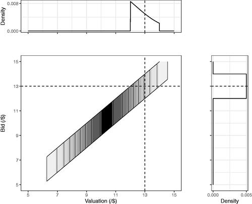
Conditional on their valuation, bidders over- and under-bid in equal numbers. For example, among those valuing the show at $13, bids are centered around $13 (see the right-hand panel). But conditional on their submitted bid, bidders are not equally under and over bidding (except those bidding the central value). In the example, among those bidding $13 more valued the show below $13 than above $13 (see Figure 1, top panel: overbidding:underbidding among those bidding $13 is around 2:1). Provided there were enough tickets that those bidding $13 were successful, two thirds of that tranche of winners overpaid what they thought the show was worth.²

While, given a particular bid of $13, the valuation held by the bidder cannot be identified from that information alone, the distribution of valuations which $13 bidders held can be modeled and therefore a reasonable adjustment for the winner’s curse can be made—in this example, the expected valuation is around $12.50. So, given some information about the distributions involved, the bidders’ expected underlying valuation can be estimated.

The Winner’s Curse in RCTs

The winner’s curse arises wherever there is a set of measurements with error. For example, a set of studies in which effect size estimates come from two distributions—a set of latent effect sizes and error (coming from random allocation). Conditional on estimates being above the mean of the distribution of estimated effects, they are likely to be overestimates of their latent value.

If a stereotypical, large RCT is conducted where there is a latent effect size $\delta ,$ the point estimate of the effect size $d$ is the result of both the impact of the difference in treatments and the effect of random allocation to groups.³ This is an unbiased estimate in the sense that $\mathbb{E}(d-\delta \mathrm{ }|\mathrm{ }\delta )=0:$ if a large number of identical studies were conducted, the mean point estimate $d$ would be close to the latent effect size $\delta .$

However, considering $d$ given $\delta$ is rarely of direct policy or research value when looking at a set of completed studies: if the latent effect size is known, it is not particularly useful to know what values the estimates might take. Of more value is estimating $\delta$ given $d:$ i.e., when the estimates are known, what can be said about the latent effect sizes?

The winner’s curse is a consequence of considering a set of RCTs in the same way as in the auction. Consider a collection of RCTs with a distribution of $d$s, each a point estimate of some latent effect size $\delta ,$ where the $\delta$s themselves are drawn from some distribution. For a given $d,$ the underlying $\delta$ might be larger than d if the realized random allocation had an effect in the opposite direction, or smaller if it had an effect in the same direction. In general $d\sim \mathcal{N}(\delta ,\mathrm{se})$ where se is the standard error associated with the random allocation of the sample. Figure 2 simulates the situation and illustrates the extent of the winner’s curse.

Figure 2. The contour plot of the joint density of $\delta$ and $d$ for a set of simulated studies. The right panel shows a density plot for $p(d|\delta =.6);$ the top panel for $p(\delta |d=.6),$ with the black area illustrating the probability that the estimate and latent effect size have opposite signs. This simulates a large set of studies with underlying latent effect sizes $\delta \sim \mathcal{N}(0,.5)$ and each study estimate $d\sim \mathcal{N}(\delta ,.25).$

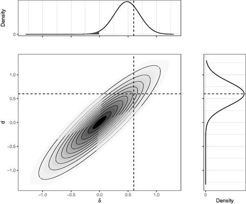
As expected, this shows $\mathbb{E}(d-\delta \mathrm{ }|\mathrm{ }\delta )=0:$ $d$ is an unbiased estimate of $\delta$ for a given $\delta$ (Figure 2, right panel). In the simulation illustrated, the mean of the estimated effect sizes of all the studies conducted where the underlying, latent effect size is known to be 0.6 is 0.6. However, $\mathbb{E}(d-\delta \mathrm{ }|\mathrm{ }d,d>0)>0$ — conditional on $d$ positive, there is an inflation effect.⁴ In the simulation illustrated, among all the studies reporting $d=.6$ (Figure 2, top panel), the expected underlying latent effect size $\delta$ is .48. That is, the expectation is the estimate is inflated 25% above the latent value. Moreover, around 1.5% of the latent effect sizes are negative (shaded in the top panel); that is, there is a small chance that a study in the collection reporting an effect size of +0.6 is a study of a negative effect.

Type M and S Errors

Gelman and Carlin (2014) introduces “type S” (sign) and “type M” (magnitude) errors, defined as the probability of a point estimate $d$ having opposite sign to its latent effect size $\delta ,$ and the mean ratio of $\frac{d}{\left|\delta \right|},$ respectively; both being conditional on $\delta ,$ on the standard error of $d$ and on $d$ being significantly greater than zero. Gelman and Carlin (2014) examines a study reporting a statistically significant effect size which appears very large given the context (sex ratios of human births). The study had large standard errors (or, equivalently, was underpowered for a small effect size) and from this, the presence of large type S and M errors was inferred.

If the latent effect size is small and a study is underpowered for it (i.e., the study has a relatively large standard error), statistical significance can only be achieved when the effect of random allocation compounds the small latent effect size. Thus, the point estimate will be an overestimate. That is, type M and S errors are inevitable consequences of assumptions: to begin an analysis with the assumption that a study is underpowered (or equivalently, that the latent effect size is much smaller than the reported estimate), is to assume a magnitude error and an increased sign error.

For example, Gelman and Carlin (2014) argues previous studies on human sex ratios had consistently shown effect sizes around $\frac{1}{8}$ th of the estimate in the study being critiqued; therefore the example study’s type M error must be around 8.

Type M error analysis, then, is similar to studying the right-hand panel in Figure 2. That is, addressing the values $d$ might take if $\delta$ is known—the value the estimated effect size from the study might take if the latent, true effect size is known. In the illustrated simulation, each study has .67 power to detect an effect size of .6 (with $\alpha =.05$); that is among the set of studies for which the latent effect size $\delta =.6,$ 67% are expected to report statistical significance. The mean of those significant point estimates is .74 suggesting type M error around 1.23.⁵ However, it is not clear that saying something about the estimate when the latent value is already known is of much practical consequence.

Often the more interesting policy question is, given a reported effect size within a set of studies, what is the distribution of latent effect sizes from which it might have come. In particular, how inflated might the estimate be and what is the chance that the reported effect size estimate is in the opposite direction to the latent effect size? This involves the equivalent of examining the top panel in Figure 2. To move from considering the right-hand panel to considering the top panel requires estimating the marginal distribution of $\delta$ from the distribution of d and this can provide a mechanism for adjusting for the winner’s curse.

Adjusting for the Winner’s Curse

In the two simulated examples above, it is possible to adjust for the winner’s curse since we know the distributions involved. Recently, published techniques for adjusting estimates of effect size to account for the winner’s curse more generally are detailed across a trio of articles (van Zwet & Cator 2021; van Zwet & Gelman, 2022; van Zwet et al., 2021). The approach bears many similarities to empirical Bayes meta-analysis (Raudenbush & Bryk, 1985).

The simulation behind Figure 2 is a simplification to aid the illustration: all standard errors are equal, as if each study has identical design including sample size. A real set of studies would not generally have standard error independent of $\delta$ and $d$— indeed, the usual purpose of power analysis is to design studies with standard errors dependent on $\delta$ and $d$ by, for example, recruiting to an appropriate sample size. It is for this reason funnel plot diagnostics are poor evidence for the presence of publication bias in meta-analyses, despite their prevalence in education research: they check for a relationship between $d$ and standard error. While publication bias might cause this, so would an intelligent research community designing studies powered for estimated effect sizes (Terrin et al., 2003).

However, we can consider two quantities which factor out the standard error: $$\zeta =\frac{\delta }{\mathrm{se}},\hspace{0.25em}z=\frac{d}{\mathrm{se}}.$$

Here $\zeta$ can be thought of as the latent signal-to-noise ratio with $z$ as its estimate from the RCT (or as the z score of the effect size, scaled by the standard error). They capture much that is of interest in the usual analysis of such a trial.⁶ For example, a study is statistically significant (with $\alpha =.05$) if $\left|z\right|>1.96$ and the (two-sided) power of the study is determined by (1) $$\Phi (-1.96-\zeta )+1-\Phi (1.96-\zeta )$$(1) where $\Phi$ is the standard normal cumulative distribution.

Given a set of studies with some appropriate properties, the distribution of $\zeta$ can be estimated from the empirical distribution of $z$ and, from that, the extent of the winner’s curse calculated and used to adjust the estimates. Such a set of studies needs to be unaffected by publication bias, file drawer problems or p-hacking. It needs to have some basic distributional assumptions: the standard error and $z$ independent, the distribution of $z$ symmetric around zero and a known distribution of $z$ given $\zeta .$

With these assumptions, if z can be modeled by a mixture of normal distributions, the distribution of $\zeta$ can be obtained from the deconvolution of that mixture with the unit normal distribution. That is, as with the simulations above, one can adjust for the winner’s curse.

This process is best illustrated using a particular set of studies in which these assumptions appear to hold.

An Illustrative Example in Education

The EEF is an independent charity in the UK established in 2011 with the aim of eliminating links between income and academic achievement. It has spent over £350 m (around $470 m, the majority from UK government sources) to run a number of initiatives including a toolkit⁷ and guidance reports. Most of the funding is used for “projects”—evaluations of educational interventions, normally with large scale RCTs, in realistic educational contexts with “business as usual” comparison treatments. While the EEF requests outcome measures are national tests, some evaluations use other standardized tests, but in general the measure is a relatively distal one (in the sense of Ruiz-Primo et al., 2002). These studies are often very expensive; for example, the implementation and evaluation of a program for parents aimed at improving student literacy cost over £500,000 (around $670,000; Husain et al., 2018). These properties—active comparisons, distal measures, and often heterogenous samples—will tend to result in relatively small effect sizes (Simpson, 2017).

The EEF sets clear standards for research groups conducting evaluations. Protocols and statistical analysis plans are normally produced in advance of the study; there is a standard template for final evaluation reports and, crucially, all reports (and protocols etc.) are lodged on a publicly available website (educationendowmentfoundation.org.uk).

As of March 2021, the EEF had published 106 study reports of randomized controlled trials in education. For this analysis, the effect size ($\mathrm{d}$) of the main result (taken to be the first result reported in the executive summary), the standard error (se), and the researcher’s claimed minimum detectable effect size (MDES) indicated in the protocol⁸ was obtained. From the first two, the value for $z$ for each study was calculated. The EEF’s approach to transparency means the set of reports has no file drawer or publication bias problems and the statistical analysis plans mitigate against p-hacking or the “garden of forking paths” (Gelman & Loken, 2014).

The assumptions required to adjust effect sizes using van Zwet’s method are that standard error and $z$ are independent, the distribution of $z$ is symmetric around zero and distribution of $\mathrm{z}$ given $\zeta$ is known. As expected from the argument above, there is a strong relationship between absolute effect size and standard error ($r^2=.27,$ $p<.0001$) despite the EEF’s publication policy ensuring no publication bias; however, there is no such relationship between z and standard error (${\mathit{r}}^2=.0001,\mathrm{\hspace{0.17em}}\mathrm{p}=.91).$

While the distribution of signed $z$-scores in the EEF data set is already close to symmetric around zero, this may only be evidence of the problem of finding effects when conducting large scale evaluation studies in realistic settings with distal measures and active comparison treatments.

In general, the analysis of RCTs is symmetrical—a trial of treatment A against treatment B is also a trial of B against A. While researchers tend to label the treatment they believe will result in better outcomes as the “intervention” and the other “control,” the labels could as easily be assigned by the flip of a coin. So, while the mean effect size from a set of RCTs would be expected to be positive as a result of the researchers’ choice of labels (provided their beliefs are generally borne out), there is no problem with relabeling. 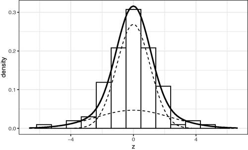Indeed, since most of the analysis involves $\left|z\right|$ and $\left|\zeta \right|,$ the discussion follows van Zwet et al. (2021) in using the symmetrized distribution⁹ (illustrated in Figure 3).

Figure 3. Histogram of symmetrized observed $z$ scores for studies in the EEF set with the fitted mixture model (solid black line) and its two components (dashed).

Finally, given the studies are all RCTs and result are scaled by the standard error, the distribution of the study estimates z given the latent signal-to-noise ratio $\zeta$ is known: $z\sim \mathcal{N}(\zeta ,1).$ So, the EEF set of project studies fits the assumptions required for estimating and adjusting for the winner’s curse.

Estimating the Extent of the Winner’s Curse in the EEF Studies

To easily estimate the distribution of $\zeta ,$ the distribution of $z$s is modeled as a mixture of normal distributions centered at zero, with standard deviation greater than 1. The mixture model ensures that the important effect of fatter tails in a set of studies is captured (Azevedo et al., 2020). For the EEF set of studies, the best fit is a mixture constructed of two normal components centered at zero.¹⁰ Table 1 shows the proportions of those two components in the mixture model of $z$ (column 1) and their standard deviations (column 2). The standard deviations of the components of the modeled distribution of $\zeta ,$ the latent signal-to-noise ratios, are calculated from deconvolutions of the components for the model of the distribution of $z$ with $\mathcal{N}(0,1)$ (column 3). Figure 3 shows the components and mixture model for the distribution of $z.$

Table 1. Components of models of distribution of $z$ and $\zeta .$

	Proportions	z	$\zeta$
Component 1	0.28	2.40	2.19
Component 2	0.72	1.06	0.37

Having constructed a model for the distribution of $\zeta$ one can calculate the exaggeration ratio (the proportion by which an observed value $z$ might be expected to overestimate the latent signal-to-noise ratio $\zeta$), the probability of a sign error (latent and observed effect sizes being in opposite directions) and estimated power across the set of studies.

Exaggeration Ratios

As noted above, the $\zeta$ associated with a particular z cannot be fully identified, but the argument allows the construction of a model of the marginal distribution of z as mixtures of normal distributions and, as $z\sim \mathcal{N}\left(\zeta ,1\right),$ the conditional distribution of latent signal-to-noise ratios $\zeta$ given the observed estimates z can be constructed and thence the distribution of $\frac{\left|z\right|}{\left|\zeta \right|}$ for a given $z$ 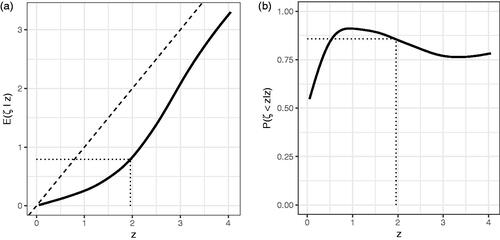can be calculated. The quartiles of the conditional distribution of this ratio, for given z is illustrated in Figure 4.

Figure 4. Median, 25th, and 75th percentiles of the distribution of the exaggeration ratio $\frac{\left|z\right|}{\left|\zeta \right|}$ conditional on $z.$

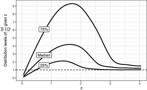
The expected latent signal-to-noise ratio $\zeta$ given $z$ can be estimated from the model. This is illustrated in Figure 5a and shows that for a barely significant result (z = 1.96), the mean $\zeta$ is .79; that is, barely significant results can be adjusted for the winner’s curse by shrinking estimates by a factor of 2.47. Figure 5b illustrates the probability that $\zeta$ < z for different values of z, suggesting that for barely significant results, there is over an 85% chance the estimated value is higher than the latent value.

Figure 5. Mean signal-to-noise ratio and probability of exaggeration, given z.

Sign Errors

Recall Figure 2 showed that conditional on a given $z>0,$ there is a chance $\zeta <0.$ That is, the estimated value from the study has opposite sign to the latent signal-to-noise ratio (and hence that the estimated effect size has opposite sign to the latent effect size). Clearly, when $z$ is close to zero, the chance of a sign error is close to .5, but even for statistically significant studies there is a chance of a sign error. Figure 6 shows that, for the EEF studies, the risk of sign error tails off as $z$ increases, but given a study which is barely statistically significant, the estimated risk of a sign error is not negligible (around .16).

Figure 6. The probability that the latent effect is in the opposite direction conditional on $z.$

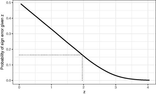
While this may appear to conflict with the intuition from the standard analysis of RCTs with type I and II errors where (if $\mathrm{\alpha }=\mathrm{ }0.05$) there is a 5% chance of a sign error, such intuition comes from treating a study in isolation. In this analysis, a study is considered as a member of a set: “we must view the … trial as a “typical” RCT in the sense that its signal-to-noise ratio is exchangeable with that of the other RCTs in the … database” (van Zwet et al., 2021, p. 6124). Conditional on it being a positive member of that set and being barely significant, there is a much higher risk of a sign error.

Power

In planning their studies, EEF researchers usually determine a MDES and design their study accordingly, normally aiming for a power of .8 to detect that MDES. The MDES can be considered as the researchers’ lower estimate of the latent effect size in the context of their study.

In the EEF reports there are different approaches to determining MDES. In some cases, sample size is beyond researchers’ control: power calculations work from a pre-determined sample size to assess study sensitivity, estimating the MDES for that sample size (given type I and II error rates $\alpha$ and $\beta$).¹¹ For example, the EEF project evaluating a mathematics mastery program (Vignoles et al., 2015) required schools prepared to convert to using a new curriculum (and also to risk their conversion being delayed if they were assigned to the RCT’s comparison arm) so sample size was set by the curriculum provider’s recruitment.

Generally, however, researchers work in the other direction if they can. Rather than using a pre-set sample size to estimate MDES, they decide on a MDES to determine sample size. Cohen (1988) argues this a priori approach “must be at the core of any rational basis for deciding on the sample size to be used in an investigation” (p. 14). There are different approaches to determining MDES, including using a pre-set standard, converting the (raw) smallest effect of interest to standardized effect size or considering effect sizes from previous studies.

For example, EEF findings are accompanied by a “security” rating. One criterion for the highest rating is MDES no higher than .2 (EEF, 2019). Many EEF researchers thus power their study using MDES = .2 (e.g., Husain et al., 2018). Alternatively, a small number of studies make reference in their power calculations to whether an effect is large enough to be educationally relevant: for example, Speckesser et al. (2018) notes “the sample size was chosen in relation to … an improvement of approximately 1/3 of a GCSE¹² grade” (p. 11).

In other cases, researchers make explicit use of previously reported effect sizes to justify MDES. This might come from widely drawn evidence; for example, in the evaluation of a social and emotional learning program, Sloan et al. (2018) refers to meta-analyses of the impact of previous social and emotional learning programs on academic performance. MDES may derive from previous studies of the same intervention, perhaps at a previous stage of the evaluation process. For example, Robinson-Smith et al. (n.d.) notes “At the piloting stage … the positive effect sizes of parents’ self-efficacy regarding discipline and boundaries and child cognitive self-regulation were .51 and .44, respectively” (p. 16).

Inevitably the practicalities of implementation affect power of the evaluation: studies under- or over-recruit, or parameters estimated prior to the study (such as intra-cluster correlation coefficient) are discovered to be different in the data. Thus, the power of the study at analysis might differ from that planned, but $\frac{\mathrm{MDES}}{\mathrm{se}}$ is a reasonable approximation for the researchers’ beliefs about latent signal-to-noise ratios; applying equation (1)(1) $$\Phi (-1.96-\zeta )+1-\Phi (1.96-\zeta )$$(1) above gives the distribution of the researchers’ belief in the power of their studies. For the EEF studies, the estimated power based on the researchers’ choice of MDES is illustrated in Figure 7a.

Figure 7. Comparison of predicted power and estimated actual power.

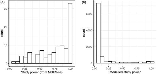
The calculations above model the distribution of $\zeta ,$ the latent signal-to-noise ratios, determined from the actual study results. Figure 7b shows the achieved power from a sample of 10,000 simulated studies from the modeled $\zeta$— that is, what power would have been achieved if the signal-to-noise ratios are the latent ones calculated here, rather than the researchers’ beliefs. The median power from the EEF researchers’ beliefs was .83, the median power of simulated studies for the modeled latent signal-to-noise ratios is .06 with only around 6% of the simulated studies having power above .8.

The Impact on Effect Sizes

Since $$\frac{\left|d\right|}{\left|\delta \right|}=\frac{\left|d\right|/\mathrm{se}}{\left|\delta \right|/\mathrm{se}}=\frac{\left|z\right|}{\left|\zeta \right|}$$ the exaggeration ratio for effect sizes is the same as that for signal-to-noise ratios. That is, it is possible to estimate the latent effect size $\mathrm{\delta }$ for each study, by multiplying $\mathrm{d}$ by the mean exaggeration ratio associated with the study’s $z$ value. Figure 8 shows the outcome of this adjustment for the 106 studies in the EEF project set.

Figure 8. Effect sizes in the set of EEF studies, against their adjusted size.

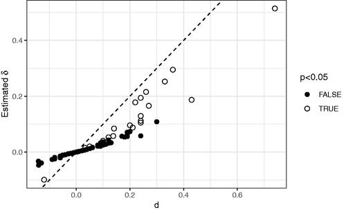
A number of features are of interest: statistically significant studies, and most of those with larger estimated effect size, grossly overestimate the latent effect size and that overestimate is not a simple scaling across the set, because the studies vary in levels of precision. As shown in Figure 5a, more precise estimates of effect size are likely to be less inflated than less precise ones.

As a result, in some cases the order of the effect sizes can be reversed. For example, while the evaluation of Butterfly Phonics (Merrell & Kasim, 2015) reports a larger point estimate of effect size $(d\mathrm{ }=.43)$ than Graduate Coaching Program ($d=.36,$ Lord et al., 2015), the less precise estimate of the former means it is likely to be more inflated. The analysis suggests the expected latent effect sizes are in the reverse order (.19 against .30 respectively). What is less clear from Figure 8 is the extent of the sign error. Among those studies which are statistically significant, the mean sign error is .14 and there is around a 50% chance that there are more than 3 sign errors among the 20 significant findings.

These inflation rates are considerably higher than those calculated by van Zwet and Gelman (2022) for a set of psychology studies and a set of phase III medical trials, where estimated mean exaggeration ratios for barely significant results were 1.7 and 1.15, respectively, reflecting that these sets probably consist of studies with much higher power to detect their latent effects.

Limitations

This analysis naturally has limitations. First, it may not currently be widely applicable: the EEF data set may be rather unusual in education in coming with strong evidence that it is free from publication bias and has statistical analysis plans that mitigate against p-hacking and other research practices which might undermine the distributional assumptions.

The exaggeration ratio and hence the extent to which an estimated effect size should be shrunk depends on the choice of set to which the study is deemed to belong. A particular study’s adjustment depends on assuming it would have latent effect size drawn from the same distribution as the set as a whole (in van Zwet & Gelman’s [2022] terms, they need to be exchangeable on the basis of the set inclusion criteria). The narrow variance of MDES among the EEF studies suggests the research community expects similar latent effect sizes; the nature of the EEF’s strategy ensures the set is complete and self-contained; and the designs, context, and study populations in the set are similar, so the EEF studies form a reasonable context for analysis.

However, if a particular study was considered as part of a different set, a different adjustment might arise. The adjustment comes from thinking of the evidence in the set as a whole, not of the information in each study separately. The high inflation factor in this analysis appears to be the result of the EEF projects having many studies with very small latent effect sizes, partly due to the decision to choose distal measures, active controls and often heterogenous samples. A different set, using different inclusion criteria and particularly with cherry-picked studies, or pre-filtered by publication bias could give smaller inflation factors, but might also be a less justifiable basis for adjustment.

Discussion

One aim of the “evidence-based education” movement is to act as a filter, primarily for policy but also for further research. On the basis of promise shown within a set of studies, further studies are commissioned, or policy is recommended. Such promise is often at least partly based on having higher effect sizes: that is, by appearing to be “winners.” Even if the set of studies from which winners are chosen is free from publication bias and p-hacking, above average results are likely overestimates and noisy above average results are likely gross overestimates. The mechanism developed by van Zwet and colleagues (van Zwet & Cator 2021; van Zwet & Gelman, 2022; van Zwet et al., 2021) gives a basis for adjusting effect sizes in a set of studies and, when applied to a well-known and highly respected set of RCTs, suggests that barely significant results should be shrunk by 60%. Moreover, even if ceteris paribus arguments do all of the heavy lifting required of them to allow effect size to be used as a measure of relative effectiveness, some interventions with higher, but noisier, effect sizes could rationally be judged as less effective than others with smaller, more precise, effect sizes.

The Winner’s Curse and Power Analysis

Effect size plays a key role in study design through power analysis. The evidence here can be read as suggesting the set of EEF projects is a collection of very underpowered studies: the median MDES predicted by the researchers was .2 but among modeled latent effect sizes only around 4% have magnitude above .2. However, one’s reading of this can be mediated by the approach to determining MDES.

A study primarily designed to detect the presence of an effect with the smallest educational value (in the context of the study) are somewhat immune from the winner’s curse, since the emphasis is on detection rather than estimation. Few EEF studies appear to have been designed this way, but in such cases, a study is perhaps not best described as “underpowered,” since failure to detect an effect for which it was properly powered provides some warrant for the absence of an effect of educational value. To describe such a study as underpowered is tantamount to arguing the designers were wrong: that smaller effects should be considered of educational value. For example, one might argue that an impact below 1/3 of a GCSE grade (used by Speckesser et al., 2018) would be of considerable educational value but it is harder to maintain this study was “underpowered” simply because it failed to detect a signal weaker than the one it was intended to detect.¹³

Similarly, for studies designed around MDES set to a standard effect size (such as the EEF’s .2), where MDES is determined by external constraints or where MDES is chosen from previous research, one might also argue that failure to reach statistical significance is not necessarily a sign that they are “underpowered” but instead as some level of evidence that any effect was not likely to be of the size intended by the researchers.¹⁴

However, if inference of the presence of an effect is based on relative effect size across a set, the winner’s curse will have an impact. For example, when many studies are carried out powered for a particular effect size and filtered for further phases of research on the basis of statistical significance,¹⁵ some will get through the filter even though the latent effect size was below the MDES (and some may even get through the filter with the wrong sign).

Power analyses which use previous research to determine MDES need to be particularly aware of this. If the set of that previous research is self-contained and complete, then the mean will be unbiased (the winner’s curse and the loser’s curse balance out). If attention is disproportionately given to a higher part of the set—perhaps publication bias filtered some studies out, or the MDES is chosen at the upper quartile—then the winner’s curse will apply: the latent effect size will be less than the MDES and the study will likely be underpowered. In particular, if an intervention is chosen for further study from among a number of possible candidates on the basis of a previous effect size, then that effect size is likely inflated.

Again, choice of set matters. For example, seen against the background of phonics interventions, Butterfly Phonics’ effect size may not seem particularly large (Merrell & Kasim, 2015). But many phonics interventions are studied with more specifically chosen participants from homogenous populations, with highly proximal measures. Once the notion that effect size is somehow a property of the intervention—rather than the study as a whole—is abandoned, one can see why an EEF evaluation of Butterfly Phonics should not be read solely in the context of a set of phonics studies, but in the context of the EEF studies. As an EEF study, the use of active comparisons, more heterogenous samples and particularly distal measures means latent effect sizes will be expected to be much smaller, and so significant effect sizes more exaggerated.

As well as attending to the set, using effect size in planning future studies needs to account for the nature of the study. If a replication is not exact, designers also have to account for the study differences when estimating MDES. An aim of the EEF is to evaluate programs in the most realistic contexts with widely drawn populations, active comparisons and national tests (which are likely to be less well related to the impact of the difference in treatments): ideal conditions for small latent effect sizes. So, the transition from pilot to efficacy to effectiveness studies would be expected to come with substantially reduced latent effect sizes at each stage, even if all interventions were taken forward without filtering. Given that the transition does also involve filtering, it will suffer the winner’s curse where latent effect sizes might be expected to be very much smaller again than those previously reported.

The analysis above suggests that expected latent effect sizes in the EEF studies are well below the effect sizes the researchers intended to detect. A way of minimizing the impact of the winner’s curse is to be more realistic about the power of studies. This might mean accepting that simple RCT designs with relatively heterogenous populations, active comparison treatments and weakly aligned measures will tend to have much smaller effects than the EEF’s standard .2 and valuable research resource may continue to be wasted if researchers continue to search for effect sizes too large to be justified. Increasing sample sizes to have a good chance of detecting small latent effect sizes will often be impractical. Redesigning studies to increase the latent effect size by targeting interventions on more homogenous groups or using more proximal outcome measures might allow for studies with acceptable sample sizes to be well powered, even if this comes at the expense of the realistic contexts EBE researchers would prefer.

Policy

While the winner’s curse has implications for designing future studies, it also impacts the filtering of studies for policy, whether that filter is statistical significance or any similar mechanism which disproportionately draws attention to a set of studies with higher values. Young et al. (2002) outlines a number of models of the process by which policy makers and knowledge generators interact. Their “knowledge driven model,” in which the role of policy makers is to implement whatever research findings are passed to them, is unlikely to be common in education. The relationship is more likely to be in the other direction: policy makers seeking to solve a problem either surveying existing research on potential solutions for the best outcome, or commissioning studies of various interventions, from among which the best are chosen. This is arguably the reason for the existence of the EEF in the UK, the Investing in Innovation (i3) and Education Innovation and Research (EIR) grants in the US and similar organizations.

This approach again results in a set of evidence which is filtered on the basis of an outcome measured with noise—prime conditions for the winner’s curse. Seemingly more successful interventions might be the result of lucky randomization and thus have inflated effect sizes, with noisier studies which get through the filter being likely to suffer more inflationary effects.

The approach taken by Gelman and Carlin (2014)—type M and S errors—considers how we can adjust for one particular study in the context of a prior understanding concerning the “true” value of the parameter. That may be useful to policy makers in helping them avoid overreacting to one surprisingly successful study and perhaps encouraging them to be a little bit Bayesian, but policy makers seeking evidence for good interventions are unlikely to already know the true values. Indeed, policy makers are often faced with a wide array of evidence from which to select a set of policies, rather than deciding whether or not to implement a particular isolated policy. In this case, they may naturally look to relevant interventions which seem to score highest on the metrics they value. While policy making is likely to be more involved than choosing on highest effect size, it is a driver behind key documents such as high profile practice guides (e.g., Fuchs et al., 2021; Hodgen et al., 2018). Even if all that involves is drawing attention away from interventions whose evaluations resulted in lower or middle effect sizes, the winner’s curse will arise. The analysis here not only reinforces that, when selections on higher size are made, measures of those chosen are likely overestimates, but shows that one can adjust for the exaggeration in the context of the set of potential policies and can identify circumstances in which an intervention with a lower, less noisy value might be preferred.

Of course, when the metric that is valued is effect size, these arguments can only come after accounting for the complexities in reasoning that an apparent positive causal role played by an intervention in the context of a study will transport to policy and practice (Cartwright & Hardie, 2012) and somehow convincingly showing that all the ceteris paribus arguments needed to make effect size a reasonable measure of relative effectiveness do really hold (Simpson, 2017). Once all that is done, knowledge of the winner’s curse and mechanisms for adjusting estimates may help policy makers avoid apparently successful studies becoming a recipe for disappointment.

Open Research Statement

This manuscript was initially submitted prior to April 1, 2022, the date that the Journal of Research on Educational Effectiveness mandated the disclosure of open research practices. Therefore, the authors were not required to disclosure their open research practices for this article.

Notes

1 The effect size which would result from perfectly matched groups instead of randomly allocated ones (or, equivalently, the limit as the sample size tends to infinity).

2 There is a complementary phenomenon: those bidding below the mean valuation are more likely to have underbid their own valuation. In the example, if there is enough supply that even those bidding $7 get tickets, two thirds of them will underpay even what they felt the show was worth.

3 Some methods texts mistakenly describe random allocation as maximizing the likelihood of two matched groups, balancing the groups or canceling out the effects of imbalanced features (e.g., Connolly et al., 2017; Hanley et al., 2016; Haynes et al., 2012; Torgerson & Torgerson, 2008). Randomization determines a well-defined probability distribution for the mean difference in outcomes from random allocation alone, and it is the addition of this distribution which leads to the winner’s curse.

4 And conditional on d negative, there is a deflation effect—the loser’s curse.

5 In this case, the type S error is very small: the chance of a study reporting a statistically significant result is in the opposite directions is around .008.

6 Assuming large enough sample size that the $t$ distribution is close to normal.

7 A widely used but unfortunately highly misleading set of meta-analyses which ignores the issues outlined above of effect size comparability, so that unsurprisingly types of intervention for which clear studies are easy to design (such as feedback) are misleadingly rated as more effective than interventions where clear studies are hard to conduct (such as extending school time) (Simpson, 2017).

8 If this was not clear in the protocol, the relevant reference to MDES in the full report was used.

9 $\left|z\right|$ matched pairwise on size and assigned opposite signs randomly within each pair.

10 Based on minimum BIC. A sensitivity analysis showed no substantial change of results with three components, with a random sample of 90% of the set or a different pattern of symmetrization.

11 In some cases, EEF evaluations note that this leads to poorly powered studies. For example, McNally (2014) were constrained on the number of schools they could work with, leading to a larger than expected MDES and the concern that the “trial is thus potentially underpowered for the small effects we are likely to obtain” which raises the question of value for money of the trial.

12 General Certificates of Secondary Education, national examinations for 16-year-olds in England.

13 In designing such detection studies, however, one needs to be careful to decide on the smallest effect of interest relevant to the study’s particular design and context: it is not enough to say that .2 is “educationally significant” in some absolute sense (Jerrim, n.d.). Identical interventions will have latent effect size well above or well below .2 depending on design choices and contextual features such as the outcome measure, the comparison treatment and the group’s heterogeneity.

14 Lortie-Forgues and Inglis (2019) argue that there is generally rather poor evidence in the EEF studies either in favor of, or against the presence of an effect. However, the argument centers on the assumption that the EEF researchers ought to have been looking for effect sizes much smaller than those the researchers themselves claimed they were looking for. So, the lack of “informativeness” suggested in Lortie-Forgues and Inglis’s analysis was an inevitable consequence of the odd way the authors defined “informative” without reference to researchers’ aims.

15 The EEF has flagged some projects as promising or for further funding which are far from statistically significant (e.g., Stokes et al., 2018), but normally interventions are flagged as promising if they are statistically significant.

References

- Azevedo, E. M., Deng, A., Montiel Olea, J. L., Rao, J., & Weyl, E. G. (2020). A/B testing with fat tails. Journal of Political Economy, 128(12), 4614–4672. https://doi.org/10.1086/710607
- Capen, E. C., Clapp, R. V., & Campbell, W. M. (1971). Competitive bidding in high-risk situations. Journal of Petroleum Technology, 23(06), 641–653. https://doi.org/10.2118/2993-PA
- Cartwright, N., & Hardie, J. (2012). Evidence-based policy: A practical guide to doing it better. Oxford University Press.
- Cohen, J. (1988). Statistical power analysis for the behavioral sciences (2nd ed.). Lawrence Erlbaum Associates.
- Connolly, P., Biggart, A., Miller, S., O’Hare, L., & Thurston, A. (2017). Using randomised controlled trials in education. Sage.
- Education Endowment Foundation. (2019). Classification of the security of findings from EEF evaluations.
- Fuchs, L. S., Newman-Gonchar, R., Schumacher, R., Dougherty, B., Bucka, N., Karp, K. S., Woodward, J., Clarke, B., Jordan, N. C., Gersten, R., Jayanthi, M., Keating, B., & Morgan, S. (2021). Assisting Students Struggling with Mathematics: Intervention in the Elementary Grades (WWC 2021006). National Center for Education Evaluation and Regional Assistance (NCEE), Institute of Education Sciences, U.S. Department of Education. http://whatworks.ed.gov/.
- Gelman, A., & Carlin, J. (2014). Beyond power calculations: Assessing type S (sign) and type M (magnitude) errors. Perspectives on Psychological Science: A Journal of the Association for Psychological Science, 9(6), 641–651.
- Gelman, A., & Loken, E. (2014). The statistical crisis in science. American Scientist, 102(6), 460. https://doi.org/10.1511/2014.111.460
- Hanley, P., Chambers, B., & Haslam, J. (2016). Reassessing RCTs as the “gold standard”: Synergy not separatism in evaluation designs. International Journal of Research & Method in Education, 39(3), 287–298. https://doi.org/10.1080/1743727X.2016.1138457
- Hattie, J. (2009). Visible learning: A synthesis of over 800 meta-analyses relating to achievement. Routledge.
- Haynes, L., Goldacre, B., & Torgerson, D. (2012). Test, learn, adapt: Developing public policy with randomised controlled trials. Cabinet Office-Behavioural Insights Team.
- Hedges, L. V. (1982). Estimation of effect size from a series of independent experiments. Psychological Bulletin, 92(2), 490–499. https://doi.org/10.1037/0033-2909.92.2.490
- Higgins, S. (2018). Improving Learning: Meta-analysis of Intervention Research in Education. Cambridge University Press.
- Hodgen, J., Foster, C., Marks, R., & Brown, M. (2018). Evidence for review of mathematics teaching: Improving mathematics in key stages two and three. Education Endowment Foundation. https://educationendowmentfoundation.org.uk/public/files/Publications/Maths/EEF_Maths_Evidence_Review.pdf.
- Husain, F., Wishart, R., Marshall, L., Frankenberg, S., Bussard, L., Chidley, S., Hudson, R., Votjkova, M., & Morris, S. (2018). Family skills: Evaluation report and executive summary. Education Endowment Foundation.
- Jerrim, J. (n.d.). Chess in school: Protocol. Education Endowment Foundation.
- Kirk, R. E. (2001). Promoting good statistical practices: Some suggestions. Educational and Psychological Measurement, 61(2), 213–218. https://doi.org/10.1177/00131640121971185
- Lord, P., Bradshaw, S., Stevens, E., & Styles, B. (2015). Perry Beeches coaching programme: Evaluation report and executive summary. Education Endowment Foundation.
- Lortie-Forgues, H., & Inglis, M. (2019). Rigorous large-scale educational RCTS are often uninformative: Should we be concerned? Educational Researcher, 48(3), 158–166. https://doi.org/10.3102/0013189X19832850
- McNally, S. (2014). Hampshire Hundreds: Evaluation report and executive summary. Education Endowment Foundation.
- Merrell, C., & Kasim, A. (2015). Butterfly phonics: Evaluation report and executive summary. Education Endowment Foundation.
- Prentice, D. A., & Miller, D. T. (1992). When small effects are impressive. Psychological Bulletin, 112(1), 160–164. https://doi.org/10.1037/0033-2909.112.1.160
- Raudenbush, S. W., & Bryk, A. S. (1985). Empirical Bayes meta-analysis. Journal of Educational Statistics, 10(2), 75–98. https://doi.org/10.3102/10769986010002075
- Robinson-Smith, L., Merrell, C., Stothard, S., & Torgerson, C. (n.d.). EasyPeasy trial protocol. Education Endowment Foundation.
- Ruiz-Primo, M. A., Shavelson, R. J., Hamilton, L., & Klein, S. (2002). On the evaluation of systemic science education reform: Searching for instructional sensitivity. Journal of Research in Science Teaching, 39(5), 369–393. https://doi.org/10.1002/tea.10027
- Simpson, A. (2017). The misdirection of public policy: Comparing and combining standardised effect sizes. Journal of Education Policy, 32(4), 450–466. https://doi.org/10.1080/02680939.2017.1280183
- Sloan, S., Gildea, A., Miller, S., & Thurston, A. (2018). Zippy’s Friends: Evaluation report and executive summary. Education Endowment Foundation.
- Speckesser, S., Runge, J., Foliano, F., Bursnall, M., Hudson-Sharp, N., Rolfe, H., & Anders, J. (2018). Embedding formative assessment: Evaluation report and executive summary. Education Endowment Foundation.
- Stokes, L., Hudson-Sharp, N., Dorsett, R., Rolfe, H., Anders, J., George, A., Buzzeo, J., & Munro-Lott, N. (2018). Mathematical reasoning: Evaluation report and executive summary. Education Endowment Foundation.
- Terrin, N., Schmid, C. H., Lau, J., & Olkin, I. (2003). Adjusting for publication bias in the presence of heterogeneity. Statistics in Medicine, 22(13), 2113–2126.
- Torgerson, D., & Torgerson, C. (2008). Designing randomised trials in health, education and the social sciences: An introduction. Palgrave Macmillan.
- van Zwet, E. W., & Cator, E. A. (2021). The significance filter, the winner’s curse and the need to shrink. Statistica Neerlandica, 75(4), 437–452. https://doi.org/10.1111/stan.12241
- van Zwet, E., & Gelman, A. (2022). A proposal for informative default priors scaled by the standard error of estimates. The American Statistician, 76(1), 1–9. https://doi.org/10.1080/00031305.2021.1938225
- van Zwet, E., Schwab, S., & Senn, S. (2021). The statistical properties of RCTs and a proposal for shrinkage. Statistics in Medicine, 40(27), 6107–6117. https://doi.org/10.1002/sim.9173
- Vignoles, A., Jerrim, J., & Cowan, R. (2015). Mathematics mastery: Primary evaluation report. Education Endowment Foundation.
- Young, K., Ashby, D., Boaz, A., & Grayson, L. (2002). Social science and the evidence-based policy movement. Social Policy and Society, 1(3), 215–224. https://doi.org/10.1017/S1474746402003068