A framework to minimise total energy consumption and total tardiness on a single machine

Abstract

A great amount of energy is wasted in industry by machines that remain idle due to underutilisation. A way to avoid wasting energy and thus reducing the carbon print of an industrial plant is to consider minimisation of energy consumption objective while making scheduling decisions. To minimise energy consumption, the decision maker has to decide the timing and length of turn off/turn on operation (a setup) and also provide a sequence of jobs that minimises the scheduling objective, assuming that all jobs are not available at the same time. In this paper, a framework to solve a multiobjective optimisation problem that minimises total energy consumption and total tardiness is proposed. Since total tardiness problem with release dates is an NP‐hard problem, a new greedy randomised multiobjective adaptive search metaheuristic is utilised to obtain an approximate pareto front (i.e. an approximate set of non‐dominated solutions). Analytical Hierarchy Process is utilised to determine the ‘best’ alternative among the solutions on the pareto front. The proposed framework is illustrated in a case study. It is shown that a wide variety of dispersed solutions can be obtained via the proposed framework, and as total tardiness decreases, total energy consumption increases.

Keywords:

• energy efficient production planning
• sustainable/green manufacturing
• multiobjective GRASP
• single‐machine scheduling

1. Introduction

This paper proposes a framework to obtain a set of efficient solutions that minimises the total energy consumption and total tardiness of jobs on a single machine. The framework utilises a metaheuristic to determine a set of non‐dominated solutions, and then an analytical hierarchy process (APH) to select the most suitable solution which will be implemented on the shop floor.

The increase in price and demand for petroleum and other fossil fuels, together with the reduction in reserves of energy commodities, and the growing concern over global warming, have resulted in greater efforts toward the minimisation of energy consumption. In the USA, the manufacturing sector consumes about one‐third of the energy usage and contributes about 28% of greenhouse gas emissions. To produce one kilowatt‐hour of electricity, two pounds of carbon dioxide is released into the atmosphere, thus contributing to global warming (The Cadmus Group 1998).

In many facilities, it is common to see that some of the non‐bottleneck machines are left running idle. For example, in a Wichita, KS aircraft supplier of small parts, manufacturing equipment energy and time data were collected at a machine shop of four CNC machines using the framework described in Drake et al. (2006). Although this machine shop is considered as the bottleneck by the production planning department, it was observed that in an eight‐hour shift, on average a machine stays idle (i.e. it is not actively processing a part, or a setup is not performed) 16% of the time. This corresponds to a 13% energy savings if the machines are turned off during the idle periods. It is observed that leaving the non‐bottleneck machines idle is considered as a normal operating practice (Twomey et al. 2008).

As a result, research in minimisation of energy in a manufacturing environment using operational methods might provide significant benefits in both reduced costs and environmental impacts. The proposed framework can be applied to any production setting and may save a significant amount of energy while keeping a good service level in terms of scheduling and energy consumption objectives. In addition, using this algorithm, the industry may leave a smaller signature on the environment, thus, leading to more environmentally friendly production planning.

To ensure energy efficient production planning, Mouzon et al. (2007) proposed dispatching rules to minimise energy consumption as well as maximum completion time for a single machine dynamic scheduling problem. It is observed that if the interarrival time until the next job is longer than a breakeven duration, then turning off the machine until the arrival of the next job provides significant energy savings. Furthermore, when production is postponed and jobs are processed without having any idle time, the energy consumption may decrease. Mouzon et al. also investigate the effects of batching on energy consumption and maximum completion time of orders: although batching increases the total completion time, it decreases the number of setups and idle time. As a result batching reduces the total setup energy and the idle energy. The dispatching rules proposed by Mouzon et al. have a great potential for reducing energy consumption especially in non‐bottleneck machines.

Energy efficiency has been an area of interest especially in portable devices such as mobile phones and laptops, which utilises embedded mobile systems (Swaminathan and Chakrabarty 2003). For example, to reduce energy consumption, hardware and software methods (Wu et al. 2006) as well as wireless protocols (Tiwari et al. 2007) are developed.

In this paper, our goal is to devise an algorithm that is capable of finding a well‐spread near optimal pareto front in a reasonable amount of time and of providing the scheduling manager with a set of non‐dominated solutions to choose from in order to minimise total tardiness and total energy consumption objectives simultaneously. The problem we are solving has not been examined in the literature to the best of our knowledge. This algorithm will provide alternative solutions that may save a significant amount of energy cost while maintaining a good scheduling service level.

The scheduling objective that is considered is the total tardiness (lateness of the tasks) objective which is a widely used measure of performance in the manufacturing environment. This objective can be defined as , where d_j is the due date of job j and c_j is the completion time of job j. Total tardiness is the sum of all jobs' lateness over the scheduling horizon. If the job is on time or early, then the associated tardiness is zero. It is also assumed that jobs are processed without preemption. Furthermore, the jobs may have non‐zero release dates (i.e. r_j ⩾0). Note that the total tardiness problem with non‐zero release dates on a single machine is considered an NP‐hard problem (Lenstra et al. 1977, Sen et al. 2003). In other words, there is no algorithm to solve this problem in polynomial time. As a result, our problem which has the total tardiness problem as one of its objectives is also NP‐hard.

It is well known that metaheuristics such as tabu search, genetic algorithm, simulated annealing, etc., can be utilised to obtain ‘good’ solutions in a reasonable amount of time for very hard problems. In this paper, the method used to solve the scheduling problem is the Greedy Randomised Adaptive Search Procedure (GRASP). An extensive review of the GRASP heuristic can be found in Resende (1998) and Resende and Ribeiro (2002). The goal of a heuristic in multiobjective optimisation is to obtain an estimation of the pareto optimal front which represents the non‐dominated solutions to the problem.

This paper is organised as follows: first, the problem definition is presented. Then, the mathematical model of minimising total energy consumption and total tardiness on a single machine with unequal release dates is developed. Next, a multiobjective GRASP is proposed. After developing the Analytical Hierarchy Process to select the best solution from the pareto front, the framework is illustrated via computational experimentation and a case study.

2. Problem definition

The multiobjective optimisation problem of minimisation of total tardiness and total energy consumption on a single machine with unequal release dates is NP‐hard, since minimisation of total tardiness on a single machine with unequal release dates is NP‐hard (Lenstra et al. 1977). To fully define the problem, the characteristics of the machine must be determined: assume that when the machine stands idle, it consumes Power _idle . Furthermore, the power consumed while processing a part is Power _processing . When the machine is turned off and then turned on (i.e. a setup occurs), it consumes Energy _setup . This setup operation takes at least T_setup duration.

The tip power, which is the marginal power utilised to process a part, must also be determined. That is,

Finally, the breakeven duration (T_B ) is defined as the least amount of duration required for a turn off/turn on operation (i.e. time required for a setup) and the amount of time for which a turn off/turn on operation is logical instead of running the machine at idle. Mathematically,

To identify solutions to the multiobjective problem that minimises total energy consumption and total tardiness, several factors must be considered in making scheduling decisions: first, the order of jobs and their starting times (or completion times) must be determined. Second, whether or not there will be a setup between two consecutive jobs must be decided. Finally, the length of the setup or length of the idle time must be determined.

The complexity of this problem can be illustrated on a two jobs example. Assume that job 1 has a processing time of 2 seconds and job 2 has a processing time of 1 second. Also, assume that job 1 has a zero release date while job 2 has a release date of 4 seconds. Finally, job 1 and 2 have a due date of 3 seconds and 6 seconds, respectively. The processing power and idle power consumptions are 2 hp and 1 hp, respectively. The setup energy is 1.5 hp.sec and the setup time is 2 seconds. As a result, T_B is 2 seconds.

Figure 1 illustrates a few feasible solutions to the multiobjective problem by considering the two possible job sequences and whether or not there is a setup between them. The first observation is that the solution that minimises the total energy consumption (solution 4) is not the solution that minimises total tardiness (solution 2). Therefore, the two objectives are conflicting. In addition, the example illustrates that when two jobs do not directly follow each other (i.e. there is an idle period between jobs), a decision relative to whether leaving the machine idle or performing a setup is necessary. This decision is based on the time between completion time of a job and the start time of the following job, and the energy consumption characteristics of the machine.

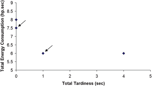
In this instance of the problem, there are two non‐dominated solutions. The feasible solutions are represented in Figure 2 and the pareto front is highlighted.

Figure 1 Feasible and non‐dominated solutions to the 2 jobs problem.

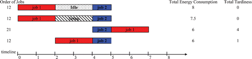
Figure 2 Non‐dominated solutions to the 2 jobs problem.

This paper proposes a framework to select the most appropriate solution from a set of non‐dominated solutions for the problem of minimisation of total energy consumption and total tardiness on a single machine. This framework involves two phases: once the set of all efficient (non‐dominated) solutions are identified via a multiobjective GRASP, a decision maker must determine the most appropriate solution to implement using a method like the APH (Saaty 1980).

3. A mathematical model for minimisation of total energy consumption and total tardiness

The Multiobjective Total Energy Total Tardiness (MOTETT) optimisation problem can be defined as:

The energy consumption objective, Equation (1) is the sum of the total idle energy (i.e. energy consumed when the machine is not processing any job) and total setup energy (i.e. the energy necessary to turn on and turn off the machine). Note that the total processing energy () is not included in the optimisation problem, since it is a fixed constant regardless of the sequence. The second objective involves the total tardiness objective, equation (2). In the mathematical formulation, equation (3) states that a job cannot be processed before it is released. equation (4) ensures that two jobs cannot be processed at the same time. Finally, equation (5) states that if a job j precedes a job k and if a setup will be performed (since the idle duration is longer than the breakeven duration), then y_jk is equal to the corresponding idle energy minus the setup energy.

By solving this mathematical model, the goal is to obtain a pareto front that will have solutions containing information about when each job should start (or finish), when to turn off and on the machine and when to leave the machine idle.

MOTETT is not linear but can be transformed into a linear mixed integer optimisation problem. Since the total tardiness problem with release dates is an NP‐hard problem, it is not practical to solve the multiobjective model using optimisation software to determine the optimal pareto front. In the next section, a multiobjective greedy random adaptive search heuristic to solve MOTETT is proposed. The advantage of metaheuristic methods is that they may provide a good solution in a reasonable amount of time. Also, these heuristics are very efficient when rescheduling is needed because of changes in the manufacturing environment.

4. Solution to MOTETT via a greedy randomised adaptive search procedure

The GRASP is a two‐phase iterative metaheuristic. First, a solution is created in the construction phase, and then the neighbourhood of this solution is locally searched to obtain a better solution. In GRASP, it is very important to define a ‘suitable’ neighbourhood in the local search phase to converge to a near‐optimal solution quickly.

The GRASP has been applied to several scheduling problems: for example, it can solve a job shop scheduling problem to minimise the total completion time effectively (Binato et al. 2000, Aiex et al. 2001). In another application, it is utilised to minimise total earliness (Laguna and Velarde 1991). It is also applied to minimise total tardiness on a single machine with setup times (Armentano and Araujo 2006). Although there are a significant number of GRASP applications to solve combinatorial optimisation problems, utilising this procedure in a multiobjective programming is not very common (Jones et al. 2002). An example of a multiobjective GRASP involves the multiobjective knapsack problem (Vianna and Arroyo 2004).

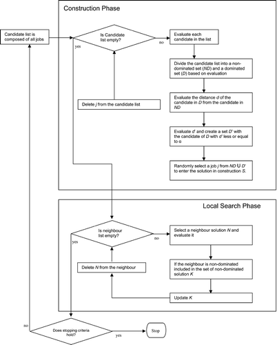
To solve MOTETT, the single objective GRASP algorithm is adapted to the multiobjective case. The multiobjective GRASP to minimise total energy total tardiness (GRASPTETT) considers a pareto front to evaluate the objectives instead of a single objective function value. The proposed GRASPTETT algorithm can be seen in Figure 3. The pseudo code below represents the GRASP algorithm:

GRASPTETT Algorithm

 While stopping criteria not satisfied

  CONSTRUCT a candidate solution s

  Do a LOCAL SEARCH around the candidate solution s.

Figure 3 GRASPTETT, a multiobjective GRASP algorithm.

The GRASPTETT algorithm runs for a predetermined number of iterations or for a maximum CPU time and it converges to a near optimal pareto front. The details of the GRASPTETT algorithm are discussed below.

4.1 Evaluation of a solution

Before describing the details of the GRASPTETT algorithm, first, how to evaluate solutions generated either at the construction phase or at the local search phase will be presented. Input to evaluating the solution procedure is a partial solution that provides the order of jobs and the setup vector, which indicates if there is a setup between consecutive jobs.

Before providing details on how to evaluate a partial solution, the total tardiness objective which is not linear has to be linearised. To linearise this objective the following transformation is used:

When a partial solution is given, the order of jobs and the setup sequence is known. As a result, MOTETT can be written as a multiobjective linear problem (MOTETTLP) as:

where Ω is the number of setups and X () is a set that contains j if there is no (a) setup between the job at position j and the job at position j+1. In this formulation, R_j , D_j, P_j and C_j denote the release date, due date, processing time and completion time, respectively, of the job scheduled at the j^th position. The MOTETTLP can be solved by combining the two objectives into a single objective by adding the weighted sum of both objectives, i.e. the objective function for the weighted problem is

This mathematical program is a linear problem. For any pair of weight combinations, a set of non‐dominated solutions for that particular job sequence and setup vector can be obtained (Steur 1986).

4.2 Construction phase

The construction phase has the objective of building a solution by adding one element at a time from a candidate list. At each iteration of the first phase, a candidate job is added to the current solution by selecting randomly a job from a restricted candidates list (RCL). The elements of the RCL are obtained from a list of non‐dominated jobs. In addition, some of the dominated jobs are also added to RCL to provide some randomness in the construction phase. The construction phase can be summarised as follows:

CONSTRUCTION Procedure

Φ = Current solution = Ø

γ = Candidate List = {1, …, n}

Non‐dominated candidate list = Ø

Dominated candidate list = Ø

While γ≠Ø

Evaluate all ι∈γ with/without setup

If ι with/without setup non‐dominated

then ι with/without setup ∈ CONSTRUCT Non‐dominated candidate list

else ι with/without setup ∈ CONSTRUCT dominated candidate list

Find distance between members of CONSTRUCT Dominated&Non‐dominated sets

Normalize the distance

RCL =  CONSTRUCT Non‐dominated List ∪{Dominated solutions with distance ⩽α}

Select randomly a from RCL

γ = γ\{a}

Φ = Φ∪{a}

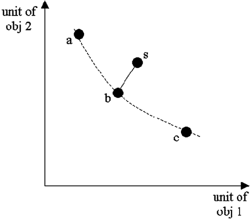
The distance of a solution from the non‐dominated set of solutions is defined by the smallest distance from a non‐dominated solution. In Figure 4, the distance between a candidate solution and a non‐dominated pareto front is the distance between s and b. The relative distance of each dominated candidate solution is divided by the maximum distance.

Figure 4 Illustration of the distance between a solution and the non‐dominated solutions.

In the construction phase, first, each candidate job must be evaluated by adding this job to the sequence with or without setup. In this evaluation, the MOTETTLP may lead to more than one solution with different lengths of idle periods or setup durations. The solutions for each candidate job are compared and the non‐dominated ones are separated from the dominated ones. In a greedy algorithm a candidate job leading to a non‐dominated solution must be chosen to be added to the current solution. But to include some randomness into the algorithm it is important to have the opportunity to add a candidate job from the dominated solution which is ‘α percent’ distant from the non‐dominated solutions. The parameter α is used to control the randomness of the algorithm: if α is equal to one then the construction phase is totally random and if α is equal to zero, then the construction phase is totally greedy.

The restricted candidates list is composed of the candidates leading to the non‐dominated solution as well as the ones leading to solutions that are at a maximum ‘relative distance’ of α from the non‐dominated solutions. Then, a candidate job is randomly selected from the restricted candidates list to enter the current solution. These steps are repeated until the current solution forms a complete solution with the order of the jobs as well as the setup vector.

4.3 Local search phase

In the second phase of the GRASPTETT algorithm, a local search is performed. Here, all of the solutions in the defined neighbourhood (N(s)), of the constructed solution s are evaluated. If the new solution is a non‐dominated solution, then it is added to the pareto set. As a result, after each iteration of the local search an approximate pareto front is obtained. This procedure can be summarised as follows:

LOCAL SEARCH Procedure

s = Current Solution

While N(s), ≠Ø

Choose y∈N(s)

If y is a non‐dominated solution

Add y to MOTETT pareto front

N(s) = N(s)\{y}

This local search for the multiobjective problem is considered similar to the single objective problem. The only difference is that instead of keeping the best solution, a set of the non‐dominated solutions is obtained. For the single objective total tardiness problem, Armentano and Araujo (2006) used two different neighbourhoods, the exchange of two jobs and the insertion of a job between two consecutive jobs. As a result, the size of each neighbourhood is n×(n−1)/2 and (n−1)². However, in this problem, each neighbour is evaluated using a series of linear programs which is very time‐consuming. To solve the problem in a reasonable amount of time, a neighbourhood with a smaller size has to be defined: new solutions are obtained by swapping the positions of two consecutive jobs [size of (n−1)] either with or without a setup, thus yielding a neighbourhood with a size of 2×(n−1) possibilities (Figure 5).

Figure 5 Illustration of the neighbourhood of a job(2). (a) Initial solution, (b) first neighbour of job 2, (c) second neighbour of job 2.

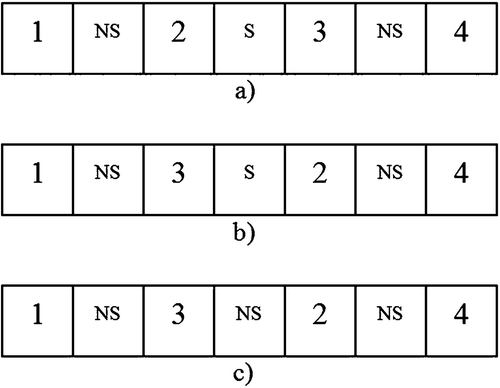
In Figure 5, two of the neighbours of solution a are represented in b and c. Job 2 and 3 are swapped and a solution with and without setup is considered as a neighbour to obtain solutions b and c . Note that solution a has six neighbours which consist of swapping jobs 1 and 2, jobs 2 and 3, and jobs 3 and 4 with and without setup.

5. Analytical hierarchy process to select best alternative from the approximate pareto front

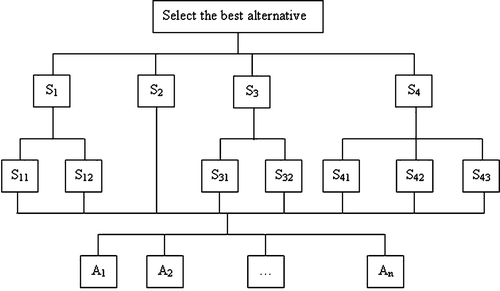
The GRASPTETT algorithm provides an approximate pareto front. To identify the ‘best’ alternative among the non‐dominated solutions on the pareto front, the decision maker can utilise his/her own preferences, which may be used as input to the APH (Saaty 1980). The AHP can choose the best alternative among a set of non‐dominated solutions. The objective is to maximise the overall purpose (top level). The decision maker must structure the problem in a hierarchy of criteria and sub‐criteria to maximise the overall purpose (top level). S/he also has to provide a pairwise comparison of the criteria to determine the value of the weight that will permit the evaluation of each alternative.

In addition to total tardiness and total energy consumption criteria, other criteria, such as maximum tardiness, total number of setups, or maximum completion time can be added. The hierarchy classification of criteria defined for this case study as an example is presented in Figure 6. The overall objective is to select the best alternative from the non‐dominated pareto front A ₁, A ₂,…, A_n . In the first level, there is energy‐related criteria (S ₁), total number of jobs not started as soon as they are released (S ₂), completion time‐related criteria (S ₃), and tardiness‐related criteria (S ₄). The first criterion (S ₁) has total energy consumption (S ₁₁) and total number of setups (S ₁₂) as sub‐criteria. The third criterion (S ₃) has total completion time (S ₃₁) and maximum completion time (S ₃₂) as sub‐criteria. Finally, the last criterion (S ₄) has total tardiness (S ₄₁), maximum tardiness (S ₄₂), and number of tardy jobs (S ₄₃) as sub‐criteria.

Figure 6 AHP hierarchy.

The decision maker needs to provide pairwise comparisons between the criteria and sub‐criteria using a scale such as the one defined by Saaty (1980) in Table 1. Assume the decision maker has defined the judgment matrix in Table 2 using Saaty's scale. According to the pairwise comparison in Table 2(a), the energy‐related criterion (S ₁) is strongly more preferred than the number of jobs not started as soon as they are released (S ₂), slightly more preferred to the completion‐time criterion (S ₃), and equally preferred to the tardiness criterion (S ₄). The completion‐time criterion is slightly more preferred to the number of jobs not started as soon as they are released. Finally, the tardiness criterion is strongly preferred to the number of jobs not started as soon as they are released and slightly more preferred to the completion‐time criterion.

Table 1. Saaty scale used for pairwise comparisons of criteria.

Scale value	Explanation
1	Equally preferred
3	Slightly more preferred
5	Strongly more preferred
7	Very strongly more preferred
9	Extremely more preferred
2,4,6,8	Used to reflect compromise between scale values

Tables 2(b) and 2(c) show that the total energy consumption is slightly more preferred than the number of setups, and the maximum completion time is slightly more preferred to the total completion time. According to Table 2(d), the total tardiness is slightly more preferred to the maximum tardiness and to the number of tardy jobs. Also, maximum tardiness is slightly preferred to the number of tardy jobs.

Table 2. AHP scaling parameters.

(a) Judgment criteria matrix (JCM).
	S 1	S 2	S 3	S 4
S 1	1	5	3	1
S 2	0.2	1	0.5	0.2
S 3	0.33	2	1	0.33
S 4	1	5	3	1
(b) Energy related JCM.
	S 11	S 12
S 11	1	3
S 12	0.33	1
(c) Completion time JCM.
	S 31	S 32
S 31	1	2
S 32	0.5	1
(d) Tardiness JCM.
	S 41	S 42	S 42
S 41	1	2	3
S 42	0.5	1	2
S 43	0.33	0.5	1

According to the preferences described above, the value judgment or priority (Δ _i) value for each alternative A_i is calculated as

where

is a scaled criterion value and □ is a criteria/subcriteria.

6. GRASPTETT parameter tuning

In this section, extensive numerical experimentation is performed to fine tune the GRASPTETT algorithm and make observations on the effect of different parameters on the performance measure that will be utilised to compare the alternative pareto fronts. Each test is run with the same parameters 10 times and the average is the measure of performance. Based on these values, the goal is to optimise the α parameter of GRASPTETT. The parameters of the problem are generated as follows: processing times are randomly generated from an exponential distribution with a mean of 3 seconds. Release dates for each job are randomly generated from an exponential distribution with a mean between arrivals of 10 seconds. Slack times (s_j ) are randomly generated from a uniform distribution with parameters 0 and where β is a parameter between 0 and 1 (Chu 1992). Finally, due dates are calculated based on the generated slack times: d_j  = s_j +r_j +p_j .

The parameter β determines how far the due dates are from the release dates. The higher the β is, the larger the available time (d_j −r_j ) to process jobs without any tardiness. Also, as β increases, the due dates are more spread over time. Parameter α allows for the inclusion of randomness into the algorithm. As noted before, when α is equal to zero, the algorithm is totally greedy and when α is equal to one, the algorithm is totally random. Values between 0 and 1 are a compromise between a totally greedy or a totally random algorithm. The algorithm is tested with α values of 0.05, 0.25 and 0.5 and problem sizes of 10, 30 and 50 jobs. The Power _idle , Energy _setup and T_setup of the machine are 1 hp.sec, 3 hp and 5 seconds, respectively. All experiments run on a Pentium core 2 Duo T7300 with 2 gigabits of RAM. The amount of time each experiment is run depends on the number of iterations that GRASPTETT runs.

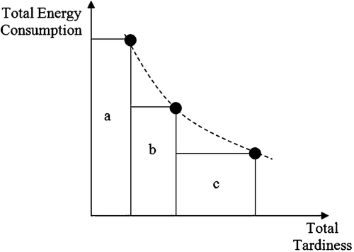
To assess and compare the GRASPTETT with different values of the parameter α, we use a ‘measure of performance’ which is the area covered by the non‐dominated set of solutions (Zitzler 1999). This area is determined by the convex union of all rectangles defined by the origin and the non‐dominated solutions. Since minimisation objectives are considered, the performance of an algorithm is better when the measure has smaller values. For example, the pareto front defined by three solutions in Figure 7, yields the union of three rectangles (a, b and c) as the measure of performance.

Figure 7 Measure of performance of a set of non‐dominated solutions.

As shown in Table 3, it seems that α is optimal at 0.5 when β = 0.05. However, as the value of β increases to 0.25 and 0.5 the optimal value for α decreases respectively to 0.25 and 0 (Tables 4 and 5). It can be concluded that as the available time to process the jobs (i.e. the slack time) increases, the optimal value for the parameter α decreases from 0.5 to 0. In other words, a totally greedy grasp algorithm will perform better when the due dates are well spread and available time between the release time and due date is large. When the slack time is small, a compromise between a random algorithm and a greedy algorithm (i.e. a β value around 0.05) will perform better. When using the algorithm on real data sets, it is helpful to first determine the average available time or slack time of the data to choose the right α level to run the GRASP algorithm.

Table 3. Performance depending on parameter α and number of jobs n with β = 0.05.

α	n = 10 (×10^3)	n = 30 (×10^4)	n = 50 (×10^5)
0	2.0344	6.8216	1.6047
0.25	1.8930	6.1498	1.4384
0.5	1.6595	5.2714	1.3776
0.75	1.7346	5.7297	1.4197
1	2.0473	5.7261	1.3824

Table 4. Performance depending on parameter α and number of jobs n with β = 0.25.

α	n = 10 (×10^3)	n = 30 (×10^4)	n = 50 (×10^5)
0	2.3726	5.5736	1.8024
0.25	2.0328	4.0509	1.5366
0.5	2.1148	3.9589	1.1883
0.75	2.5790	4.6978	1.3428
1	2.5782	4.7974	1.5283

Table 5. Performance depending on parameter α and number of jobs n with β = 0.5.

α	n = 10 (×10^3)	n = 30 (×10^4)	n = 50 (×10^5)
0	0.7941	1.8725	0.4754
0.25	0.9609	3.1914	1.3963
0.5	1.1083	3.3974	1.4135
0.75	0.8635	2.8428	1.4888
1	1.0637	2.6075	1.3641

7. Case study

This section presents a case study of 50 job problem with an exponential arrival time of 10 seconds and exponential processing times with a mean of 3 seconds. We observe that the most difficult problems have a low β value where the due dates are close to the release dates and tight. As a result, we set the parameter β to 0.05. The Power _idle , Energy _setup and T_setup of the machine are 1 hp.sec, 3 hp and 5 seconds, respectively. The GRASPTETT method is able to find the approximate pareto front in a considerable amount of time (less than 1 CPU minute) whereas an exact method would have spent a tremendous amount of time to reach the optimal solution for a 50 job problem even for the single objective one machine total tardiness problem with unequal release dates.

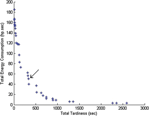
The pareto front for this case study is shown in Figure 8. Note that the processing energy is not included in the total energy consumption. Each of the solutions represents the schedule of setups as well as the start time of each of the 50 jobs. As shown, if the total tardiness cost decreases, the total energy consumption increases, which shows the trade‐off between total energy consumption and total tardiness. The set of solutions consists of an approximation of the optimal pareto front. The decision maker or the controller can then make a decision on which schedule to choose depending on his/her preference.

The AHP is applied on 10 best alternatives on the pareto front according to the priority presented in Table 6. As shown, all best solutions have the same maximum completion time (i.e. the last job in the sequence is completed at the same time in all solutions). However, the total completion time objective varies from one solution to another (approximately a range of 8% variation). The best solution (alternative 10 which is the solution pointed to with an arrow in Figure 8) has a total of four setups with a total energy consumption of 50.4 hp.sec. Also, in this solution, 38 jobs are not started as soon as they are released, and 24 jobs are tardy. However, the total tardiness is small and on average, each tardy job is 14 seconds late with a maximum lateness of 56.7 seconds.

Table 6. Case study.

Alternatives	S 11	S 12	S 2	S 31	S 32	S 41	S 42	S 43	Evaluation
1	56.4	6	37	11295.5	395.6	324.2	56.7	25.0	0.75644
2	15.0	5	44	11735.4	395.6	740.2	78.7	36.0	0.75645
3	9.0	3	46	11903.8	395.6	898.0	80.3	38.0	0.75940
4	82.9	8	31	11063.2	395.6	126.7	29.0	15.0	0.75978
5	24.0	8	42	11504.4	395.6	520.2	42.2	34.0	0.76381
6	12.0	4	45	11743.0	395.6	740.2	78.7	36.0	0.76437
7	96.7	4	30	11048.2	395.6	118.3	30.5	13.0	0.76812
8	72.8	8	31	11099.2	395.6	157.1	29.0	18.0	0.76973
9	40.3	8	38	11314.2	395.6	343.0	30.7	27.0	0.77591
10	50.4	4	38	11308.8	395.6	332.2	56.7	24.0	0.77634

Figure 8 Pareto front for 50 random jobs withβ = 0.05.

8. Conclusion

Minimising total tardiness and total energy consumption at the same time is a difficult problem that can take a large amount of time if solved to optimality. The purpose of this paper is to develop a framework to obtain an optimal set of non‐dominated solutions with different levels of energy consumption and total tardiness. The GRASP metaheuristic is used to obtain an approximate pareto front and its parameter is optimised to obtain the best results. The decision maker can then make a choice among the set of solutions or input preferences into an AHP procedure. To illustrate how the framework can be utilised, a case study is analysed.

The multiobjective optimisation problem defined in this paper has been solved using a multiobjective GRASP (GRASPTETT). To the author's best knowledge, GRASP has not been extensively utilised in multi‐objective optimisation. As a result, the GRASPTETT algorithm presented in this paper is an algorithmic contribution. In addition, minimisation of total energy consumption and total tardiness at the same time is a new class of problem that needs to be modelled and solved efficiently.

The proposed methodology can be applied to settings other than manufacturing equipment. For example, many drivers should make the difficult decision of leaving the car idle while waiting for somebody. Another example is the compressors in the industrial setting: compressors use about 50% of the maximum power when they are idle. It may be desirable to turn off the compressors instead of keeping them at the idle mode for a long amount of time. For other big energy consuming machines such as boilers, and chillers the same observation can be made.

The problem of minimisation of energy consumption and a scheduling objective at the same time is quite challenging: complexity results from the scheduling objective and also from having setups between jobs, and deciding the length of the setups and idle duration. Future work on this problem might be to extend to a multi‐machine environment. In this environment, scheduling jobs at the same time on two machines may increase the total energy bill significantly since the energy charges not only include the consumption charge but also peak demand charge. Another extension is considering equipment with multiple sleep modes (e.g. computers have stand by, hibernate and sleep modes). In this environment, one needs to decide the sleep mode of the machine and the duration of stay.

References

- Aiex , R. M. , Binato , S. and Resende , M. G. C. 2001 . “ Parallel GRASP with path‐relinking for job shop scheduling. ” . In Parallel computing ATT Labs Research Technical Report
- Armentano , V. A. and Araujo , O. C. B. 2006 . Grasp with memory‐based mechanisms for minimizing total tardiness in single machine scheduling with setup times. . Journal of Heuristics , 12 (6) : 427 – 446 .
- Binato , S. , Hery , W. J. , Loewenstern , D. M. and Resende , M. G. C. 2000 . “ A greedy randomized adaptive search procedure for job shop scheduling. Essays and surveys in metaheuristics. ” . In ATT Labs Research Technical Report
- The Cadmus Group . 1998 . Regional Electricity Emission Factors Final Report
- Chu , C. 1992 . A branch‐and‐bound algorithm to minimize total tardiness with different release dates. . Naval Research Logistics , 39 : 265 – 283 .
- Drake , R. , Yildirim , M. B. , Twomey , J. , Whitman , L. , Ahmad , J. and Lodhia , P. 2006 . “ Data collection framework on energy consumption in manufacturing. ” . In Proceedings of 2006 Institute of Industrial Engineering Research Conference May 2006, Orlando, FL
- Jones , D. F. , Mirrazavi , S. K. and Tamiz , M. 2002 . Multi‐objective meta‐heuristics: an overview of the current state‐of‐the‐art. . European Journal of Operational Research , 137 (1) : 1 – 9 .
- Laguna , M. and Velarde , J. L. G. 1991 . A search heuristic for just‐in‐time scheduling in parallel machines. . Journal of Intelligent Manufacturing , 2 : 253 – 260 .
- Lenstra , J. K. , Rinnooy Kan , A. H. G. and Brucker , P. 1977 . Complexity of machine scheduling problems. . Annals of Discrete Mathematics , 1 : 343 – 362 .
- Mouzon , G. , Yildirim , M. B. and Twomey , J. 2007 . Operational methods for the minimization of energy consumption of manufacturing equipment. . International Journal of Production Research , 45 (18–19) : 4247 – 4271 .
- Resende , M. G. C. 1998 . “ Greedy randomized adaptive search procedure (GRASP). ” . In AT&T Labs Research Technical Report 98.41.1
- Resende , M. G. C. and Ribeiro , C. C. 2002 . “ Greedy randomized adaptive search procedures. ” . In State of the Arts Handbook on Metaheuristics , Boston, MA : Kluwer .
- Saaty , T. 1980 . The analytical hierarchy process , New York : John Wiley .
- Sen , T. , Sulek , J. M. and Dileepan , P. 2003 . Static scheduling research to minimize weighted and unweighted tardiness: a state‐of‐the‐art survey. . International Journal of Production Economics , 83 (1) : 1 – 12 .
- Steur , R. E. 1986 . Multiple criteria optimization: theory, computation, and application , Malabar, FL : Krieger Publishing Company .
- Swaminathan , V. and Chakrabarty , K. 2003 . Energy‐conscious, deterministic I/O device scheduling in hard real‐time systems. . IEEE Transactions on Computer‐Aided Design of Integrated Circuits and Systems , 22 : 847 – 858 .
- Tiwari , A. , Ballal , P. and Lewis , F. L. 2007 . Energy‐efficient wireless sensor network design and implementation for condition‐based maintenance. . ACM Transactions on Sensor Networks , 3 (1) : 1 – 23 .
- Twomey , J. , Yildirim , M. B. , Whitman , L. , Liao , H. and Ahmad , J. 2008 . “ Energy profiles of manufacturing equipment for reducing consumption in a production setting. ” . In Working Paper Wichita State University
- Vianna , D. S. and Arroyo , J. E. C. 2004 . “ A GRASP algorithm for the multi‐objective knapsack problem. ” . In XXIV International Conference of the Chilean Computer Science Society 69 – 75 . 11–12 November 2004, Arica, Chile. IEEE Computer Society
- Wu , H. , Ravindran , B. , Jensen , E. D. and Li , P. 2006 . Energy‐efficient, utility accrual scheduling under resource contraints for mobile embedded systems. . ACM Transactions on Embedded Computing Systems , 5 (3) : 513 – 542 .
- Zitzler , E. 1999 . Evolutionary algorithms for multiobjective Optimization. Thesis (PhD) Swiss Federal Institute of Technology, Zurich