A modelling framework for the acquisition and remanufacturing of used products

Abstract

In recent times, there has been a consistent need for companies to produce ‘green’ products and offer ‘green’ services in order to contribute to environmental protection. The utilisation of used devices (extending their useful life cycle) is an excellent, indirect way for companies to conform to this requirement and, at the same time, increase their profit. Cell phones constitute one of the most interesting cases of products, which can be returned, remanufactured and reused: their replacement rate is large, the available quantity for reuse is huge and, consequently, the profit potential is significant. Motivated by the real case of a company involved in the acquisition and remanufacturing of used cell phones, a simple mathematical programming model is proposed in this work that can help remanufacturing companies to make optimal decisions concerning the quantities to be purchased and remanufactured. Its use, namely the simulation of the model stochastic parameters and the optimisation of the model, reveals not only that the exploitation of used products can be profitable, but also that as the ‘product acquisition system’ improves, the economic benefits for any remanufacturing company can be even greater.

Keywords:

• reverse logistics
• remanufacturing
• mixed integer programming
• cell phones/mobile phones
• product acquisition

1. Introduction

In the last two decades, companies especially in the EU and the USA have been asked to produce environmentally friendly products and offer ‘green’ services in order to contribute to the international, large-scale effort of environmental protection. One way of doing so is through the utilisation of used devices, which extends their useful life cycle. Consequently, the number of products that are reused – through any of the different options of reuse (remanufacturing, reuse of components, recycling, etc.) – is gradually increasing. This does not happen only because companies are encouraged (mainly in the USA) or mandated (mainly in the EU, e.g. by the WEEE and RoHS directives) to produce and sell ‘green’ products, but also because companies become progressively aware of the profitability of reuse activities. Undoubtedly, the environmental legislation has already started to constitute a lever, which makes companies seriously examine the development of product recovery systems. Nevertheless, in recent years it has been realised that these recovery systems should not be considered as a cost centre, but as a profit centre.

The enormous increase in research on remanufacturing (see comprehensive reviews at Guide 2000, Fleischmann 2001 and Srivastava 2007) and, more recently, on closed-loop supply chains (CLSC) is not, therefore, at all surprising. van Wassenhove and Guide (2002) focus on the business aspects of creating and managing cost-effective CLSC. They identify the most important processes required by a CLSC including product acquisition, reverse logistics, inspection (consisting of testing, sorting and grading), disposition, remanufacturing, distribution and selling. CLSC have also been studied by the European network ‘Reverse logistics and its effects on industry’, the major research results of which are gathered and presented in the volumes edited by Dekker et al. (2004) and Flapper et al. (2005). A comprehensive review and discussion of several areas in CLSC is presented by Guide and van Wassenhove (2003), while Guide et al. (2003) critically discuss important gaps in the research literature; the areas of inspection, disposition, distribution and selling of remanufactured products have not been thoroughly examined from an academic point of view. On the contrary, the operational aspects of remanufacturing have received the most attention and there have been numerous contributions dealing with production planning and control (Guide and Srivastava 1998, Guide 2000, Souza et al. 2002), inventory control (van der Laan 1997, Inderfurth 1997, van der Laan et al. 1999, Toktay et al. 2000) and materials planning (Inderfurth and Jensen 1999, Ferrer and Whybark 2001).

In general, the decision to engage in reuse activities should be made based on an integrated economic analysis of the costs and benefits of such activities. This analysis should be done even when the law mandates recovery, because it can determine the best way to manage product returns. A company that has established a product recovery system relies on returned products, since the latter constitute its raw materials. Hence, product acquisition management becomes of great importance because it can affect several essential issues: whether reuse activities are profitable; if they are, then, how profitable they can be; a number of operational issues such as facility design, production planning, control activities, etc. However, the area of product acquisition is another area of CLSC that has had a very limited amount of research, as Guide and van Wassenhove (2001) ascertain. In addition, French and LaForge (2006) arrive at the same conclusion regarding product acquisition in process industries. Nevertheless, some important contributions can still be found in the area of product acquisition. Galbreth and Blackburn (2006) point out that the condition of returned items is often highly variable and sorting is an important remanufacturing operation. They examine the case of a remanufacturer who acquires unsorted used products from third party brokers and they propose some optimal acquisition and sorting policies. A year later, Zikopoulos and Tagaras (2007) examine procurement and production decisions in reverse supply chains under yield uncertainty. More specifically, they investigate how the profitability of reuse activities is affected by uncertainty in terms of the quality of returned products. Note that our work is mostly focused on product acquisition, trying to fill in the aforementioned research gap.

Guide and van Wassenhove (2001) mention that there are two systems for obtaining used products from end-users: the waste stream system and the market-driven system. In the context of the former, companies passively accept any product return, not being able either to influence the quality of returns or to acquire returned products only of a certain quality. Inevitably, the companies involved consider the huge volumes of returned products as a costly nuisance whose losses they try to minimise. The adoption of a rather ‘chaotic’ system like this can be justified only for companies facing mandatory product returns and just for a short adjustment period, during which they should advance their product acquisition management to a higher level, after the conduction of the economic analysis mentioned before.

The market-driven system is more popular among US companies, because they have been persuaded about the profitability of reuse activities, mainly remanufacturing (Guide 2000). Besides, by building a green profile voluntarily, US companies intend to keep the national legislation loose – indirectly, of course, because ‘officially’ they cannot influence it– since, for the time being, it simply encourages and does not force them to embody any reuse activities. Usually, companies which have adopted this system motivate end-users to return used products, trying to influence the products' quality level in various ways: for example, by offering financial incentives especially for better quality used products. Overall, it is a characteristic of market-driven systems that the return rate, timing and quality of returned products are not regarded as variables of an extraneous process which cannot be controlled and influenced by the companies, but as a process with wide margins of activation.

One way or another, more and more companies find themselves either with used products in hand or with offers in batches of returned products. Many of them get involved in reuse activities and this is what makes the quantitative mathematical programming model developed in this work particularly useful. Consequently, the major objective of this paper is to propose a simple, mixed integer programming (MIP) model, which can help companies involved in remanufacturing activities to determine both the optimal quantities to be purchased and remanufactured. Moreover, we apply the MIP model in practice to prove not only the profitability of remanufacturing used products, but also the even greater profitability of an evolved product acquisition system (PAS). This double goal has been achieved first, through the simulation of the stochastic parameters of the model and, then, through the optimisation of the appropriate version of the model. Finally, we conduct sensitivity analysis (of the appropriate versions) of the MIP model, in order to find out which of the model parameters affect the optimal solution most and, thus, draw the attention of any potential user of the presented optimisation tool to their careful determination.

It should be mentioned that even if this paper focuses on the acquisition and remanufacturing of used cell phones, the proposed mathematical programming approach is general enough to be used in other production systems. The same strategy has been used by a few other researchers who focus on cell phones in order to study various remanufacturing issues. First, Seliger et al. (2004) and, then, Franke et al. (2006) develop a generic remanufacturing plan for cell phones. Their approach for the planning of remanufacturing capacities and programmes by means of combinatorial optimisation and discrete-event simulation, supports any planner in the periodic adaptation of an existing remanufacturing system. Uncertainties regarding quantity and condition of mobile phones, reliability of capacities, processing times and demand are considered. Robotis et al. (2005) model the case of a reseller who acquires used products (e.g. cell phones) of old technology from an advanced market and then he either (1) sells (a small fraction of) these used products in a developing market – where the old technology is acceptable – without any value-adding activities, or (2) adds value by remanufacturing these products to an as-new condition and then sells them in the developing market at a higher price.

The paper is organised as follows. A case of product recovery concerning a remanufacturer of cell phone units is first discussed (Section 2). Then, in Section 3 the mathematical programming model and its versions are presented, while Section 4 includes some illustrative examples. The sensitivity analysis of the proposed model is conducted in Section 5. Finally, some concluding remarks and directions for future work are presented in Section 6.

2. Problem definition

ReCellular, Inc. (www.recellular.com) was established in 1991 as a global trading operation of remanufactured, graded and used cell phones, as well as other handheld electronics. It offers remanufactured products as a high quality, cost-effective alternative to new cellular handsets. The company belongs to the cellular communications industry, which is a highly dynamic market where the demand for new telephones changes continuously for many reasons: introduction of new technology, promotional campaigns, opening of new markets, etc. At the same time, the factors that influence demand also affect the availability of used handsets: the supply of used cell phones is an unstable and volatile market (van Wassenhove and Guide 2002). The product acquisition management of ReCellular also depends on the unknown future demand for remanufactured phones. ReCellular has to purchase and keep stocks of used phones to compete for sales, as the lead times for delivery, after the acquisition agreement with its suppliers, are often lengthy and uncertain. The company does not collect handsets directly from the end-users, but obtains them in bulk mostly from airtime providers or third-party collectors, such as charitable foundations. All these may offer a variety of handsets in varying condition (quality level), for a wide range of prices and volumes. Thus, the company receives from its suppliers, almost on a daily basis, plenty of offers in batches of used cell phones of different models, quantities and quality levels1. Based on an estimated future demand for used handsets, Recellular has to decide which offers to accept and then, from every batch that is selected to be purchased, the quantities of used phones to remanufacture. All these daily decisions should be made in the context of maximising the total profit, while satisfying all operating constraints.

In the proposed mathematical model, it is assumed that ReCellular is not able, but mainly willing to influence the quality of returned cell phones and, consequently, their acquisition cost. First, it is meaningless to offer financial incentives to its suppliers in order to receive used phones of better quality, because ReCellular does not acquire handsets directly from the end-users. Second, the volatility of the market mentioned previously makes the company cautious about offering this type of financial motivation. Finally, it is more important for the company to know the quality of returned cell phones as accurately as possible, than to receive used devices of the highest quality; note that the latter is not absolutely certain that it is the most profitable potential for ReCellular. This actually depends on all the other price and cost parameters, as it will become clear through the illustrative examples in Section 4.

The PAS that is set up today between ReCellular – and generally between any remanufacturer – and its suppliers is rather immature: it includes trading of batches containing cell phones in multiple quality levels, while even the same supplier may offer batches of different quality mix from deal to deal. Besides, no acceptance sampling is carried out before the acquisition of any batch and generally there is significant uncertainty. It is interesting to mention that in the past the system was even more ‘primitive’, but enough progress has been made since then (Guide and van Wassenhove 2001). For several reasons, further evolution of the PAS should be tempting both for ReCellular and the suppliers of used handsets. Figure 1 represents the current state of the PAS (1) and the states towards which it may and should move progressively in the future (2, 3 and 4). Evidently, the higher the state of the PAS, the more mature it is.

Figure 1 The states of the PAS.

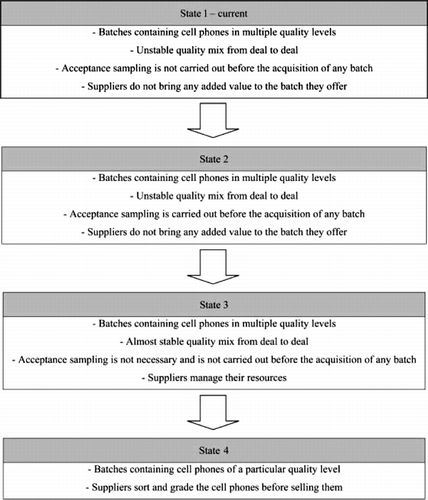
If the aforementioned evolution occurs, the expected benefit of ReCellular is evident (and can be tremendous): any remanufacturing company would clearly prefer the PAS to become more deterministic, because this would allow it to be more profitable, providing its customers with the quality they want at the lowest possible cost. Currently, Recellular may purchase cell phones of a different quality level than it would prefer and thus be burdened much more than necessary.

On the other hand, the most important incentive for suppliers to support the evolution of the PAS is their ability to make this business more profitable for them as well. The increased profitability would be the result of an increase in the prices of used cell phones; each supplier should be paid better for ‘adding value’ to any batch (for example by sorting and/or grading cell phones), before selling it and for guaranteeing less or no uncertainty at all to ReCellular. Progressively, the greater profitability of this business for any participating supplier will attract others to join the specific market. The long-term increase in suppliers will offer Recellular more alternatives, which may even further contribute to a profit increase.

3. Modelling framework

As mentioned previously the MIP model that is proposed in this Section aims at determining the optimal quantities to be purchased and remanufactured by any remanufacturing company like ReCellular, every time it receives several offers in batches of used products. Depending on the state of the PAS, the MIP model is modified accordingly; in Subsections 3.1 to 3.4 we discuss the various alternative versions of the model.

Note that Pourmohammadi et al. (2004) design a material network flow to minimise the environmental and operational costs of exchanging waste and by- product materials in a B2B network. In order to represent this problem, they formulate a mixed integer linear model. In addition, Lebreton and Tuma (2006) use the same optimisation approach in a similar CLSC case: a linear programming model is developed to assess the profitability of tire remanufacturing. Finally, Willems et al. (2006) quantify the disassembly time reductions required to achieve economic feasibility of systematic product disassembly. They use a modelling framework, based on linear programming, to investigate the effect of reducing the expected disassembly time and cost on the selection of the optimal end-of-life strategy.

The MIP model presented here is developed for a single-period setting and is related to a specific type of used products (e.g. Nokia 5100). In a particular period – deal, every supplier offers to the remanufacturing company just one batch of used products. The supplier quotes the price of the latter according to (1) the quality mix he usually offers based on all previous deals and (2) the approximate prices which used products of certain quality levels have in market (see Section 4 for more details). It is also assumed that the remanufacturing company does not try to influence either the various costs or the quantities of the offered batches, which is often a realistic assumption as in the case of ReCellular that we mentioned earlier. An estimated future demand for remanufactured products drives the remanufacturing company to order batches of used devices. As it usually happens in practice, the company has to purchase either the whole quantity of an offered batch or nothing. When acceptance sampling is conducted (state 2 of the PAS), the remanufacturing company is supposed to sample every offered batch before its potential acquisition. We also consider that there is no disposal, because returned devices can be remanufactured regardless of their initial quality level. On the other hand, every returned product needs remanufacturing in order to be sold in the secondary market: even the best quality level of products, e.g. the one corresponding to devices which have simply been out of package, is lower than the quality level of a completely remanufactured product. Finally, used products are remanufactured only if they are to be sold.

Let the index i () reflect the identity number of the supplier offering a batch of used products and the discrete random variable J , taking the values , reflect the quality level of those products. Also assume that the best quality level is L and the worst is 1. The mathematical programming formulation relies on the following parameters:

• D : estimated future demand for remanufactured products which should be satisfied at the end of the examined period;

• A _i : batch size offered by supplier i;

• p _s : selling price of a remanufactured unit;

• p _e : salvage price (corresponding to the salvage value) of an acquired, but non-remanufactured unit; it is independent of the unit quality level and the supplier who offered it. Evidently, it is ;

• c _a,i : acquisition cost of a used unit from supplier i;

• c _r,j : remanufacturing cost of a used unit at quality level j;

• c _s : shortage cost per unit of unsatisfied demand;

• c _c : sampling cost of a used unit;

• q _i : percentage of a batch offered by supplier i that is going to be sampled before the acquisition of the batch2;

• W : available budget;

• f _i ( j ): percentage of used units in the batch offered by supplier i, being at quality level j. These percentages are actually the values of the probability mass function , which are determined in practice through (1) extremely insecure estimations based, for example, on data collected from all previous deals with any supplier i, if any (state 1 of the PAS), (2) estimations based on the sampling outcome of batches (state 2 of the PAS) and (3) reliable estimations based on data collected from previous deals with any supplier i (state 3 of the PAS);

The decision variables of the model are the following:

• y _i : a binary variable which reflects the decision of the remanufacturing company to order or not the batch offered by supplier i; it is

• x _i,j : the fraction of A _i f _i (j) which should be remanufactured; it is for every i and j;

The following variables are also introduced to model the problem:

• C : total profit of the remanufacturing company, which includes the opportunity cost as well;

• A : total quantity of used units which the company should order from its suppliers. It is .

• R _j : quantity of used units being at quality level j which should be remanufactured. It is calculated by:

• R : total quantity of used units which should be remanufactured (and sold). It is

The objective function (OF) of the MIP formulation expresses the total profit, which should be maximised. It has the following form:

The first two terms of Equation (3) represent the company's revenue from selling the remanufactured units, as well as from salvaging the non-remanufactured ones, respectively. The negative terms that follow, correspond to the total sampling cost, the total acquisition cost, the total remanufacturing cost and the opportunity cost, respectively. Note that the cost of sampling the batch offered by supplier i is assumed to be proportional to the sample size q _i A _i , which, in turn, is proportional to the size A _i of the specific batch.

The OF is subject to the following constraints:

Constraints (4) ensure that if the remanufacturing company does not order the batch offered by supplier i (i.e., ), then no products could be remanufactured from this batch (i.e., for every j). Constraint (5) imposes that used products should be remanufactured only if they are to be sold and constraint (6) is auxiliary and arises as a combination of Equations (2) and (1). The MIP model can also include a budget constraint, like constraint (7).

Omitting the constant term c _s D and making some modifications, then Equation (3) becomes as follows:

where . Using Equations (1) and (2), and letting , and , then Equation (10) is further simplified:

In addition, constraints (5) and (6) should be replaced by and Equation (1) respectively.

In the above formulation, it is interesting to note that p expresses the profit from every remanufactured product, not only because it will be sold (direct profit), but also because it will not burden the company with shortage cost (indirect profit). Parameter r _j reflects the cost of every remanufactured product at quality level j: apart from the obvious remanufacturing cost, r _j reckons that any remanufactured  product will not be salvaged (indirect loss), but sold. Finally, a _i reflects the additional cost for acquiring every used product offered by a specific supplier i, since the salvage price guarantees a minimum payback for every acquired used product.

To enlighten the reader about the type of problems that can be solved with (the appropriate version of) the MIP model presented above, let us consider the following introductory information of a fictitious case: in order to satisfy an estimated future demand for 1000 remanufactured cell phones, a company involved in reuse activities examines which of the following offers to accept: a batch offered by supplier 1 of 700 used phones and/or a batch offered by supplier 2 of 1100 phones. In the following subsections, additional information regarding this example is given, which is differentiated depending on the state of the PAS examined.

3.1 State 1 of the PAS

In this state, the percentages f _i (j) of used products being at quality level j, in the batch of any supplier i, are either completely unknown, e.g. in the case of a new supplier, or significantly different from deal to deal. Consequently, although it is necessary to use certain values of those percentages for any supplier i, in order to find the optimal MIP solution of a specific deal in practice, it should not be ignored that any estimations used for this purpose are not reliable and the risk of arriving at a non-optimal solution is high.

Additionally, in state 1 of the PAS it is for any i, since no acceptance sampling is carried out before the acquisition of any batch.

In our illustrative example, using the introduced notation and the hypothetical information of all previous deals with suppliers 1 and 2 about the percentages f _i (j), we can consider that the remanufacturing company wants to satisfy a demand for phones and based on the values of the price and cost parameters (p _s , p _e , c _a,i , c _r,j , c _s ), it has to choose either the batch of phones, containing, let us say, 301 phones at quality level 3 – assuming – and 399 phones at the best quality level – assuming – or/and the batch of phones, containing, let us again suppose, 297 phones at quality level 5 – assuming – and 803 at the worst quality level – assuming . As mentioned previously, the actual quality mix of both offered batches could be slightly or completely different, a fact that renders acceptance sampling and transition to state 2 of the PAS very tempting.

3.2 State 2 of the PAS

In this more advanced state, acceptance sampling would permit the remanufacturing company to have a better idea of the percentages f _i (j). Thus, both the MIP model and the decisions about the acquisition and the remanufacturing of batches would become more accurate; they would be based on recent values of the percentages f _i (j) and not on old, and probably unreliable information about them. This means that acceptance sampling of offered batches can be extremely useful for any company involved in remanufacturing activities.

There is more than one way of conducting and handling the results of sampling. The only way to get a precise view of the quality mix of all offered batches, is by examining the whole batches (100% inspection) before acquiring any of them, which means that in this case it is for any i. A serious disadvantage of this procedure is the extremely large total inspection cost.

In our example, if the company had examined the whole batches before their potential acquisition, let us suppose that it would have found that the batch offered by supplier 1 contains 245 phones at quality level 3 and 455 phones at the best quality level, while the batch offered by supplier 2 contains 275 phones at quality level 5 and 825 at the worst quality level. Consequently, 100% inspection would have given the following results: , , and .

A simpler, faster and cheaper, but not so accurate alternative, regarding the information about the percentages f _i (j), would be to conduct random sampling in every offered batch and then use exclusively the results of sampling in order to estimate those percentages. It is well known that the main disadvantage of any sampling procedure is that in order to increase its reliability, it is necessary, among other things, to take as large a sample as possible, which means a high sampling cost. Besides, by adopting this way of handling the results of sampling, all previous data reflecting the ‘quality history’ of suppliers would not be taken into consideration. However, this is not a disadvantage at all, if the representativeness of the sampling procedure is ensured and if the reader recalls that in this particular state of the PAS, the percentages f _i (j) may be different from deal to deal.

In our example, sampling e.g. 10% of both offered batches ( for any i), i.e. 70 and 110 phones respectively, could have given the following fictitious results: 25 phones offered by supplier 1 at quality level 3 and 45 phones at quality level 6, while 28 phones offered by supplier 2 at quality level 5 and 82 phones at quality level 1. These figures would lead to the following estimations of the percentages f _i (j): , , and . Consequently, the remanufacturing company would have concluded that the batch offered by supplier 1 contains 252 phones at quality level 3 and 448 phones at the best quality level, while the batch offered by supplier 2 contains 275 phones at quality level 5 and 825 at the worst quality level.

The aforementioned disadvantages of random sampling can be mitigated by calculating a ‘weighted’ estimation, which could combine the information arising both from the current sample and previous deals. The offered quantities of used products, the age of data or a combination of them could be used as weights. However, the most effective technique to exploit the sampling procedure in order to update properly knowledge about the percentages f _i (j) is by using Bayes' theorem and the fact that regardless of the distribution of the quality level J, the sampling mean is distributed normally for large sample sizes. The disadvantages of this procedure are the following:

• Making use of past information about any supplier i is worthy only if the quality mix he offers remains relatively stable from deal to deal. Otherwise, the importance of sampling becomes crucial and past information has limited value.

• In order to take advantage of Bayes' theorem, it is necessary for the MIP model to include additional terms proportional to the mean quality level, such as , which do not exist in the particular form of the model.

3.3 State 3 of the PAS

The version of the MIP model that corresponds to state 3 of the PAS is identical to the one of state 1. However, there is an important difference regarding its accuracy, that arises from the fact that the percentages f _i (j) of all suppliers do not change considerably between successive deals. Therefore, once a remanufacturing company obtains their values after a number of deals, it can incorporate them into the MIP model, in any future deal.

In this state it is for any i, since no acceptance sampling is carried out before the acquisition of any batch.

3.4 State 4 of the PAS

Let us now consider the following variation of the initial example: in order for a remanufacturing company to satisfy an estimated future demand for cell phones, it examines which of the subsequent offers to accept: a batch offered by supplier 1 containing phones at quality level 3 and/or a batch offered by supplier 2 containing phones at quality level 5.

In this state of the PAS, the mathematical programming formulation is simplified not only because it is for every i, but mainly because for any supplier i, for only one value of J and for any other value; in our example .

4. Illustrative examples

The presented MIP model has been applied to a number of practical problems in order to show that remanufacturing may be significantly profitable. It has also been used to evaluate from an economic point of view the transition of the PAS from state 3 to 4. The profitability of the transition from state 1 to 2 or from 2 to 3 largely depends on the uncertainty of the qualities of returned products and, therefore, of the offered batches. Nevertheless, subsequently, apart from the transition of the PAS from state 3 to 4, which is mainly examined, we also discuss the transition from state 2 to 3.

The methodology that has been used comprised the following steps:

1. determination of the range of the parameters values,

2. simulation of the parameters,

3. optimisation of the appropriate version of the MIP model

4. comparison and analysis of the emerging results.

The tool that has been used in steps (2) and (3) was Microsoft Fortran PowerStation 4 and its libraries; we have developed a number of programs specifically for this particular paper. Additionally, just for the sake of verification, we have used another software combination: first we have formed the appropriate version of the MIP model at Microsoft Office Excel, then we have conducted simulation of the parameters using ‘Crystal Ball’, which is a special add-in software of Microsoft Office Excel and, finally, the MIP model has been solved using ‘Solver’ of Microsoft Office Excel.

The data that have been used in the illustrative examples were collected mainly from the web site of ReCellular and are summarised in . In the following paragraphs we explain how the presented values have been chosen.

Table 1 Characteristics and description of the various quality levels of returned cell phones.

Quality level	Description
6	Pass a functional and electrical test and with minimal cleaning look like brand new. Phones show no physical damage and have a good antenna, display, lens, keypad and a working charging system.
5	Pass a functional and electrical test and with cleaning and buffing look almost as if they were brand new. Phones show no physical damage and have a good antenna, display, lens, keypad and a working charging system. Keypad and plastic may show some fading.
4	Pass a functional and electrical test but will require rework to make these phones usable. Phones have a good display and working keypad, but may have some physical damage and may show signs of wear that will require the replacement of some parts.
3	Phones have the same physical appearance as the quality level 6 phones, but failed the test or did not power up and their lens may have some scratches. Many of these phones can be repaired with some technical knowledge.
2	Phones have the same physical appearance as a quality level 5 phones, but failed the test or did not power up. Many of these phones can be repaired with some technical knowledge.
1	Phones have failed the test or did not power up. Phones can be used for part salvage.

Table 2 Parameters values for states 3 and 4 of the PAS.

States 3 and 4
Parameter	Examined values	Parameter	Examined values	Parameter	Examined values
K	6	p s ($)	U (125, 145)	c r,4 ($)	U (30, 31.5)
i	1 to	P e ($)	U (4, 13)	c r,5 ($)	U (20, 21)
L	6	c r,1 ($)	U (45, 47.25)	c r,6 ($)	U (5, 5.25)
j	1 to	c r,2 ($)	U (40, 42)	c s ($)	U (7.5, 33.5)
D (cell phones)	U (10, 5000)	c r,3 ($)	U (35, 36.75)	W ($)	A very large value
State 3
	Examined values
Parameter	Scenario 1	Scenario 2	Scenario 3	Scenario 4	Scenario 5	Scenario 6
f i (j) for ∀ i	The types of suppliers arise randomly	Every type of supplier appears once	The types of suppliers arise randomly	Every type of supplier appears once	The types of suppliers arise randomly	Every type of supplier appears once
A i for ∀ i (cell phones)	U (0, 0.8√D)	U (0, 0.8√D)	U (0, 1.1√D)	U (0, 1.1√D)	U (0, 5000)	U (0, 5000)
State 4
Parameter	Examined values
c a,i ($)	For	For	For	For	For	For
	U (60, 63)	U (70, 73.5)	U (80, 84)	U (90, 94.5)	U (95, 99.75)	U (100, 105)
A i for ∀ i (cell phones)	for every j, where A i refers to the batch size of state 3
Note: Information on prices and costs was valid in 2004. Today, there might be significant differentiations.

The number of suppliers and quality levels of used phones is taken to be six, i.e. and . In order to determine the percentages f _i (j) that are used for the evaluation of deals made in state 3 of the PAS, each supplier is considered to have access to a different group of users; these users have different habits and the quality level of returned phones is highly dependent on how the phones are treated during their use. For example:

• A collector that purchases phones from users in Scandinavia and the airtime providers offering a 30-day return policy, provide ReCellular with uniformly high quality phones, e.g. or .

• A collector that deals with users in the USA has a very mixed collection: most phones show average wear, a few are in very poor condition (e.g. due to water damage) and a few are in like-new condition, e.g. , , , , , (the specific example is based on real data from a collector in the USA).

• A charitable foundation provides ReCellular with very high quality phones, e.g. .

• A supplier that deals with commercial contracts (where the phones may have been heavily used and not maintained, e.g. used by people in a big construction company) offers fairly poor quality phones, e.g. or .

The various types of suppliers used to illustrate the applicability of the MIP model are summarised in Table 3.

Table 3 Percentages f _i(j) of the various types of suppliers.

Type of supplier	Percentages f i (j)
I
II
III
IV
V
VI

The demand for remanufactured phones D varies uniformly between 10 and 5000 units, according to real data from ReCellular. Usually, the size of the offered batches is directly connected to the demand D, because suppliers take it into account before determining their offers. Three cases have been studied regarding the values of A _i s of state 3: in the first two ones, suppliers are assumed to take the expected demand D into account in order to determine their offers, while in the third one it is assumed that only the maximum value of D, i.e. 5000 units, is taken into consideration by the suppliers. Consequently, according to the first case (0, 0.8D), in order to take into account that often the maximum offered batch size is somewhat smaller than the estimated demand. In the second case (0, 1.1D), considering the possibility that the maximum offered batch size may be slightly greater than the demand. Finally, in the third case (0, 5000).

However, in order to evaluate the potential benefit from the transition of the PAS from state 3 to 4, it is necessary to determine simultaneously the size of the offered batches for both examined states, namely (1) the size of batches containing used cell phones at a quality mix, according to the percentages f _i (j) of any supplier i (state 3), as well as (2) the size of batches containing phones at a specific quality level (state 4). The simultaneous determination of A _i s is based on the requirement that the total offered quantity of used phones per quality level should be the same, regardless of the state of the PAS. This requirement can guarantee that the examined offers are equivalent and the results comparable. In Table 4 we present three indicative sets of batch sizes for both examined states. In these sets, first the values of all A _i s and all f _i (j)s of state 3 have been simulated – where (0, 1.1D) – and then every A _i of state 4 has been calculated using ; in this sum A _i refers to the batch size of state 3. For example, the highlighted quantity (first indicative set – state 4) arises as follows: .

Table 4 Indicative sets of size and quality of offered batches.

	State 3									State 4
D	i	A i	Type of supplier	f i (1)	f i (2)	f i (3)	f i (4)	f i (5)	f i (6)	j	A 1	A 2	A 3	A 4	A 5	A 6
1133	1	702	I	0	0	0.2414	0.2586	0.2993	0.2007	1	251.64
	2	614	II	0.0848	0.1621	0.3079	0.2921	0.1379	0.0152	2		293.19
	3	682	III	0	0	0	0	0.4720	0.5280	3			533.85
	4	760	IV	0.2540	0.2460	0.2231	0.2769	0	0	4				987.24
	5	1236	V	0	0	0	0.3365	0.3602	0.3034	5					1061.80
	6	19	VI	0.3442	0.3502	0.3056	0	0	0	6						885.27
1700	1	1251	II	0.0691	0.1955	0.3413	0.2587	0.1045	0.0309	1	510.97
	2	136	II	0.0972	0.1512	0.3186	0.2814	0.1488	0.0028	2		709.71
	3	1033	IV	0.2868	0.2132	0.2061	0.2939	0	0	3			1095.25
	4	1349	II	0.0853	0.1663	0.3054	0.2946	0.1337	0.0147	4				1410.73
	5	1094	III	0	0	0	0	0.5026	0.4974	5					1214.56
	6	1061	V	0	0	0	0.3279	0.3143	0.3579	6						982.78
2029	1	68	I	0	0	0.2071	0.2929	0.2385	0.2615	1	0
	2	1854	I	0	0	0.2595	0.2405	0.2712	0.2288	2		0
	3	1227	V	0	0	0	0.3541	0.3100	0.3359	3			984.98
	4	2109	I	0	0	0.2323	0.2677	0.2005	0.2995	4				2089.32
	5	1304	V	0	0	0	0.3657	0.3370	0.2973	5					1896.53
	6	415	V	0	0	0	0.3551	0.3248	0.3201	6						2006.17

Regarding the values of A _i s of state 4 in Table 4, it should be noted that the equivalency of offers between states 3 and 4 is achieved (1) in the first two sets if the remanufacturing company receives offers for every quality level and (2) in the third set if it receives offers for only four quality levels. Consequently, the types of suppliers participating in a deal of state 3 ‘affect’ the values of A _i s of state 4.

Coming back to the percentages f _i (j) of state 3, two cases have been studied leading to a total of six scenarios presented in Table 2. As per the first case, the types of suppliers that participate in a deal arise randomly: for example, ReCellular may receive in a deal three offers from suppliers of type I and three offers from suppliers of type V (see the third indicative set in Table 4). As per the second case, one supplier of every type offers a batch to the remanufacturing company (see the first indicative set in Table 4).

In order to determine the values of the acquisition cost c _a,i of a used cell phone according to its quality level j (state 4), first the information about the minimum sum of money that ReCellular should have paid in order to acquire a returned Nokia 5100 has been considered for all six quality levels (Table 5). Then, it has been considered that in practice c _a,i fluctuate uniformly in the interval (min c _a,i , 1.05·min c _a,i ), for any quality level j. The specific range of values is consistent with the fact that c _a,i should always be an increasing function of j. On the other hand, the acquisition cost c _a,i of a cell phone unit offered by supplier i, when the deal is made in state 3, arises taking into consideration the need for equivalency between the compared states of the PAS and the assumption mentioned at the beginning of Section 3; according to this each supplier quotes the price of the cell phones in his batch, based on the quality mix he usually offers, i.e. according to his percentages f _i (j). For example, a supplier of type I using the minimum c _a,i s of Table 5 should offer his products in .

Table 5 Minimum values of c _a,i s and c _r,j s, for a used Nokia 5100, depending on its quality level.

j	1	2	3	4	5	6
min c a,i	60	70	80	90	95	100
min c r,j	45	40	35	30	20	5

The procedure of determining the remanufacturing cost c _r,j for every quality level j is similar. The minimum remanufacturing costs c _r,j s of a used Nokia 5100 depending on its quality, according to ReCellular, are given in Table 5. In practice c _r,j fluctuate uniformly in the interval (min c _r,j , 1.05·min c _r,j ), for any quality level j.

ReCellular acquires used handsets and after their remanufacturing process, sells them at a price that goes beyond the various costs (i.e. acquisition, remanufacturing, etc.), assuring a reasonable profit for the company. Taking into consideration the fluctuation of c _r,j s and c _a,i s for all quality levels, and a reasonable profit margin for ReCellular (i.e. between 5 and 15%), it follows that the selling price p _s of a remanufactured Nokia 5100 varies uniformly between 125 $ and 145 $. Concerning the salvage price p _e of a non-remanufactured Nokia 5100, it should be noted that there is always a common value for any cell phone, regardless of its quality level. This is typically a very low value, which varies uniformly from 5 to 15% of the average acquisition price of cell phones in various quality levels.

Shortage cost usually takes the form of lost sales cost or back order cost. It includes payment of overtime and/or special administrative expenses due to stock-outs, loss of sales and loss of goodwill. In our case, the shortage cost c _s per cell phone unit of unsatisfied demand reflects a ‘lost opportunity for profit’. Therefore, using p _s and the average c _r,j s and c _a,i s for any quality level j, the shortage cost c _s has been estimated to be distributed uniformly between 7.5 $ and 33.5 $. Finally, in order to simplify the MIP model, a very large value for the available budget W has been assumed. In this way, constraint (7) becomes non-active.

Using the data of Table 2, the parameters of the MIP model have been simulated 20,000 times for each one of the six examined scenarios. Then, for each scenario and simulated set of parameters values, the appropriate version of the MIP model (between those two that correspond to states 3 and 4 of the PAS) has been optimised. In Table 6 we present a complete set of parameters values and the solution of the MIP model for states 3 and 4 of the PAS, regarding the second (highlighted) indicative set of A _i and f _i (j) values of Table 4. Note that C _m represents the optimal – maximum – total profit (OF) for states and 4 of the PAS. In every other case, the parameters have been simulated and the optimal solutions have been determined accordingly.

Table 6 Simulated parameters values and solution of the versions of the MIP model for states 3 and 4 of the PAS, for the second (highlighted) set of A _i and f _i (j) values of Table 4.

Parameters values for both states 3 and 4
p s	p e	c r,1	c r,2	c r,3	c r,4	c r,5	c r,6	c s
128.75	6.29	46.22	41.25	36.28	30.64	20.59	5.16	27.80

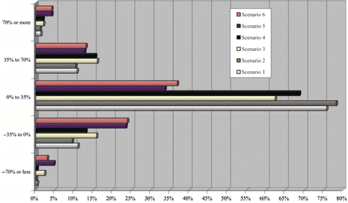
The analysis of results determines the percentage profit increase in state 4 compared to state 3, i.e. , ranks combinations according to ΔQ ₄, determines the maximum, the minimum and, mainly, the average ΔQ ₄ for every scenario, detects and enumerates cases where either or and finally creates the histogram of relative frequencies of ΔQ ₄. In Table 7 and Figure 2 we summarise the most important results for all examined scenarios. Various important conclusions can be drawn, such as:

• C ₃ or C ₄ might be negative for many reasons. The most important one is related to the combination of sizes of the offered batches, especially when every (0, 5000), which might render the decision of the remanufacturing company to order the proper set of batches exceptionally difficult: for instance, if the company has to choose between six very large (small) batches when D is very small (large), the, probably large, excess (shortage) in the optimal solution and, consequently, the negative values of C ₃ or C ₄ are unavoidable.

  Table 7 Analysis of results of all simulated sets (20,000 per examined scenario).

  	Scenario 1	Scenario 2	Scenario 3	Scenario 4	Scenario 5	Scenario 6
  Percentage (number) of sets where C 3 < 0 (%)	0 (0)	0.02 (4)	0 (0)	0.005 (1)	16.52 (3304)	16.57 (3314)
  Percentage (number) of sets where C 4 < 0 (%)	0.06 (12)	0.02 (4)	0.35 (70)	0.005 (1)	18.06 (3611)	20.80 (4159)
  Percentage of sets where ΔQ 4>0 (%)	88.89	90.91	81.05	86.61	68.73	70.83
  Average ΔQ 4 (%)	17.37	17.84	16.56	19.34	46.21	9.49
  Maximum ΔQ 4 (%)	500.62	914.49	306.83	545.89	147,832.80	180,820.45
  Minimum ΔQ4 (%)	− 175.60	− 37.22	− 234.22	− 65.92	− 212,684.21	− 80,471.09

  Figure 2 Relative frequencies of the percentage profit increase .

  

• Considering the small percentage (number) of sets where either or , the profitability of remanufacturing activities – at least in the case of used cell phones – for every company taking action in states 3 or 4 of the PAS becomes obvious. Evidently, this happens mainly when suppliers take into consideration the estimated demand D before determining their batch size (Scenarios 1–4); the increased dispersion of batch sizes regarding the actual demand D (Scenarios 5–6) raise significantly the percentage (number) of unprofitable deals.

  Parameters values for state 3						Parameters values for state 4
  c a,1	c a,2	c a,3	c a,4	c a,5	c a,6	c a,1	c a,2	c a,3	c a,4	c a,5	c a,6
  83.94	84.02	77.30	84.31	99.65	97.82	60.92	71.16	83.43	93.44	95.27	104.07

  Solution of the version of the MIP model for state 3
  y 1	y 2	y 3	y 4	y 5	y 6	C 3	A	R	R 1		R 2	R 3	R 4	R 5		R 6
  0	1	0	1	0	0	9929.45	1485	1485	128.24		244.87	455.32	435.68	200.63		20.26
  x 1,1	x 1,2	x 1,3	x 1,4	x 1,5	x 1,6	x 2,1	x 2,2	x 2,3	x 2,4	x 2,5	x 2,6	x 3,1	x 3,2	x 3,3	x 3,4	x 3,5	x 3,6
  0	0	0	0	0	0	1	1	1	1	1	1	0	0	0	0	0	0
  x 4,1	x 4,2	x 4,3	x 4,4	x 4,5	x 4,6	x 5,1	x 5,2	x 5,3	x 5,4	x 5,5	x 5,6	x 6,1	x 6,2	x 6,3	x 6,4	x 6,5	x 6,6
  1	1	1	1	1	1	0	0	0	0	0	0	0	0	0	0	0	0

  Solution of the version of the MIP model for state 4
  y 1	y 2	y 3	y 4	y 5	y 6	C 4	A	R	x 1	x 2	x 3	x 4	x 5	x 6
  0	1	0	0	0	1	30,561.99	1692.50	1692.50	0	1	0	0	0	1

• The percentage of sets where approaches (in the worst case) and exceeds (by far usually) 70%. This makes obvious that the profitability of remanufacturing activities – at least at the cellular communications industry – will become much more remarkable, if the PAS gradually evolves in the future.

• More specifically, the transition of the PAS from state 3 to 4 can ensure an average percentage profit increase ΔQ ₄ that varies between 9.49% (Scenario 6) and 46.21% (Scenario 5). When suppliers take the expected demand D into account in order to determine their offers (Scenarios 1–4) the average ΔQ ₄ is not differentiated seriously; otherwise, the average ΔQ ₄ takes more extreme values (see a more analytical remark below).

• Undoubtedly, the maximum and minimum ΔQ ₄ values are impressive, either positively (mainly) or negatively. However, those values might be misleading, especially in Scenarios 5–6, where they often arise due to extremely small absolute values of C ₃. A better idea about the distribution of ΔQ ₄ is given in Figure 2, where it is evident that in the majority of sets (for all scenarios) ΔQ ₄ varies between 0 and 35%.

• Regarding the influence of the examined scenarios (keep in mind that the various scenarios are differentiated according to the combination of the values of A _i s and the types of suppliers participating in deals made in state 3 – see Table 2 for more information) on the results, it should be noted that:

  • The bigger the potential maximum size of A _i s, i.e. moving from the pair of Scenarios 1–2 to 3–4 and, then, to 5–6, the more important the way the percentages f _i (j) are determined; when every (0, 0.8D) (Scenarios 1–2), then the types of suppliers taking part in a deal do not affect significantly the average ΔQ ₄. It remains almost stable at 17.5% at Scenarios 1–2. When every (0, 1.1D) (Scenarios 3–4) the differentiation of the average ΔQ ₄ arises at 2.78% () and finally at Scenarios 5–6 the differentiation of the average ΔQ ₄ is significant.

  • Comparing the scenarios in pairs that are determined according to the maximum value of A _i s, namely Scenarios 1 vs 2, 3 vs 4 and 5 vs 6, it seems that the single appearance of every type of supplier in a deal leads to an increase in the average ΔQ ₄, when suppliers take into consideration the estimated demand D in order to determine the size of their batches (Scenarios 1–2 and 3–4). This can be mainly attributed to the bigger uniformity of the offered batches in Scenarios 2 and 4 (in comparison with Scenarios 1 and 3 respectively), regarding the quality of used phones they contain. On the contrary, when suppliers participating in a deal ignore the specific value of D, the decrease in the average ΔQ ₄ is remarkable: from 46.21% it shrinks to 9.49%.

• By having a close look at the parameters values of Table 2, it becomes clear that all returned handsets, even those of the poorest quality, can be remanufactured profitably. Taking this into consideration, if , then the optimisation of the versions of the MIP model for states 3 and 4 of the PAS leads to the following result: and, thus, states 3 and 4 are ‘equivalent’ regardless of the examined scenario. This equivalency of states is a result of the fact that the optimal acquisition policy for the company in both states is to purchase and remanufacture every offered batch, due to the need to avoid shortage, which usually costs a lot. Consequently, there is no effect from the different style of offers that appears at the two states of the PAS.

• Studying the optimal solutions of the MIP model (for both states 3 and 4) which recommend that the company should acquire an excess of products, i.e. , and, more specifically, the optimal y _i s and x _i,j s, it can be seen that every acquired batch (i.e. ) with size is completely remanufactured (i.e. ), except for one: this batch can be considered as the one that leads to excess and contains the products with the lowest profitability. In other words, in the optimal solution when the choice of batches lead to an excess of products, one can be found at most.

Regarding the transition of the PAS from state 2 to 3, the profitability of two fictitious deals made between a remanufacturing company and its suppliers is compared; the first one is made in state 2 of the PAS, while the second in state 3. We assume that in both deals each supplier i offers a batch of size A _i , with the same quality mix of used products, described by some percentages f _i (j), which are the same for both states of the PAS. Understandably, the two deals are almost identical and, therefore, comparable. They differ only because in the case of the deal of state 3 of the PAS the company can rely on previous knowledge of the percentages f _i (j) of any supplier i, as they do not change significantly between successive deals, while in the case of the deal of state 2 the quality mix of any supplier is unstable from deal to deal and the company has to conduct acceptance sampling in order to estimate those percentages. In the ideal occasion where acceptance sampling gives absolutely accurate information about the actual percentages f _i (j) of all suppliers, then and, therefore, it will always be . In the more realistic case where acceptance sampling leads to more or less inaccurate estimations of the percentages f _i (j), sub-optimal solutions of the MIP model will be obtained, directing the remanufacturing company to improper choices of batches to acquire and remanufacture, thus in (much) lower total profit than the actual C ₂. Hence, in any case it is and this clearly reveals that the evolution of the PAS can bring important economic benefits for any company involved in reuse activities.

5. Sensitivity analysis of the proposed MIP model

Wagner (1995) states that the values of various parameters of any model are often ‘guesstimated’ and that it is usually helpful to practitioners to understand the sensitivity of a model to simultaneous variations in several parameters. Therefore, the sensitivity analysis of the versions of the MIP model corresponding to states 3 and 4 of the PAS is very interesting, since it reveals which of the price, cost and all other parameters affect the optimal solutions and, generally, the examined models most; thus, any potential user of the presented optimisation tool will be careful in their determination.

At first, regarding the sensitivity analysis of the version corresponding to state 3, only Scenarios 1, 3 and 5 (where the types of suppliers arise randomly) have been examined. Accordingly, in state 4 of the PAS it has been assumed that the quality level of cell phones offered by each supplier arises randomly.

The sensitivity analysis has been carried out in the following steps:

1. determination of the range of the parameters values (already done in Section 4 – presented in Table 2),

2. specification of the sensitivity analysis methodology,

3. simulation of the parameters and optimisation of the appropriate version of the MIP model

4. analysis of results.

As far as the sensitivity analysis methodology is concerned, the one proposed by Wagner (1995) has been implemented. Among the three alternative algorithmic methods that he presents, ‘Monte Carlo estimation of parameter sensitivity’ has been selected in order to ascertain the relative influence of the model parameters.

Considering the version of the MIP model for state 4, it can be easily observed that 22 parameters can vary, i.e. A _i and c _a,i for , c _r,j for , as well as p _e , p _s , c _s and D. All these imprecise parameters affect the OF and some of them affect constraint (6) as well. Since all A _i s (as well as c _a,i s and c _r,j s) are equivalent, the sensitivity analysis of the specific version of the model in relation to the variation of just one A _i (c _a,i and c _r,j ) is enough in order to find out the impact of the variation of any other A _i (c _a,i and c _r,j ).

A final remark about the implemented sensitivity analysis methodology is that due to the fact that the 22 aforementioned imprecise parameters vary jointly, the one-at-a-time sensitivity notion has been considered as a more precise indicator of global sensitivity. Wagner (1995) mentions that this notion is good at discerning the parameters that influence strongly any examined model. The following steps have been followed:

• One (at a time) of the imprecise parameters has been considered as known. This has been the conditioning parameter, p _k , which has been sampled times.

• For each one of these 200 sampled values of p _k , the remaining (21) parameters have been sampled times simultaneously.

• For each one of the 2000 combinations of parameters values, for and , namely the optimal total profit for state 4 of the PAS and for specific values of s and t, has been determined.

• Considering the values of for each one of the 200 values of p _k at a time (i.e. for a specific value of s at a time), averages of have been calculated from the following formula: for .

• Then, for the residuals have been calculated from the following formula: for a specific value of s at a time and for .

• The value of has been estimated as the sample variance of the residuals, using the following formula: , and indicates the variation in the optimal total profit due to the joint variation in all the other (21) parameters, given only the value of p _k .

• The variance of C ₄, namely , has been estimated using

• The results have been transformed in terms of R ² through the following formula: , where is the fraction of variation in C ₄ attributable to the conditioning parameter p _k .

The only difference that can be detected at the sensitivity analysis of the version of the MIP model corresponding to state 3 of the PAS is that in this case there are 58 imprecise parameters, i.e. f _i (j) for and , A _i and c _a,i for , c _r,j for , p _e , p _s , c _s and D, instead of the 22 imprecise parameters that can be found in state 4.

The sensitivity analysis results are summarised in Table 8. Given that (1) the larger the value of , the more p _k influences the variation of the OF and (2) if is greater than , then the OF is more sensitive to p _k than p _j , we conclude that among the imprecise parameters, it is by far the demand D and, secondarily, the selling price p _s of a remanufactured cell phone unit that influence the MIP model the most. All the other parameters affect the model much less and almost equally. This conclusion arises regardless of the examined state of the PAS and the distribution of A _i s. The only influence that can be detected when either of them differentiates can be connected with the variances and , i.e. in the variability of the profitability of the remanufacturing activities. More specifically,  <  regardless of the distribution of A _i s, while both and take greater values when every (0, 5000).

Table 8 Sensitivity analysis results.

State 3 of the PAS
Parameter	A i ∼U (0,0.8 · D) for ∀ i			A i ∼U (0,1.1 · D) for ∀ i			A i ∼U (0,5000) for ∀ i
pk
D	258,763,383	1,082,154,241	0.761	249,572,475	1,080,533,105	0.769	358,669,007	1,449,807,024	0.752
p s	779,692,298	1,111,688,993	0.299	742,674,849	1,053,212,235	0.295	1,184,331,686	1,443,883,475	0.180
c r,l	1,005,355,673	1,107,093,637	0.092	978,309,736	1,074,738,905	0.090	1,335,099,947	1,476,648,192	0.096
p e	966,423,504	1,076,390,633	0.102	990,370,778	1,093,970,751	0.095	1,220,606,022	1,367,246,360	0.107
A 1	992,941,324	1,108,368,535	0.104	965,640,030	1,067,453,614	0.095	1,317,229,625	1,465,259,837	0.101
c s	981,608,690	1,083,460,186	0.094	994,308,866	1,121,898,848	0.114	1,315,678,443	1,469,309,489	0.105
c a,1	994,128,215	1,097,968,916	0.095	926,580,868	1,058,031,262	0.124	1,348,510,094	1,474,993,274	0.086
f 1 (1)	1,027,458,816	1,118,222,793	0.081	996,277,426	1,115,125,018	0.107	1,265,413,351	1,446,481,406	0.125
State 4 of the PAS
D	308,533,125	1,400,620,596	0.780	345,769,300	1,430,516,877	0.758	421,860,626	1,799,455,068	0.766
p s	1,050,585,023	1,362,280,021	0.229	1,086,742,658	1,414,279,087	0.232	1,396,072,048	1,750,699,754	0.203
c r,l	1,182,036,654	1,322,757,713	0.106	1,219,267,454	1,371,204,625	0.111	1,527,408,214	1,684,166,299	0.093
p e	1,237,974,191	1,396,584,295	0.114	1,291,006,353	1,442,749,324	0.105	1,532,141,662	1,700,168,011	0.099
A 1	1,258,830,823	1,387,059,062	0.092	1,289,017,532	1,434,714,469	0.102	1,523,152,641	1,678,719,323	0.093
c s	1,262,408,580	1,406,859,253	0.103	1,274,173,372	1,408,864,239	0.096	1,444,289,156	1,615,289,036	0.106
c a,1	1,219,522,421	1,357,697,529	0.102	1,248,086,922	1,380,093,339	0.096	1,604,543,173	1,820,829,228	0.119

It should be noted that the aforementioned conclusions concerning the influence and, consequently, the importance of the imprecise parameters on the MIP model remain the same even when every type of supplier (Scenarios 2, 4 and 6 – state 3 of the PAS) and every quality level (state 4 of the PAS) appears once, when simulating the parameters of both states during the sensitivity analysis. Therefore, ReCellular and any other remanufacturing company of the cellular communications industry should be extremely careful in the determination of D and p _s , in order to use the MIP models properly and reliably.

6. Conclusions

This work presents a basic MIP model and a number of alternative versions, which are suitable for the various states of the PAS that is set up between a remanufacturer and its suppliers. These models aim at determining the optimal quantities to be purchased and remanufactured by (re-)manufacturing companies, every time they receive offers in batches of returned products. The illustrative examples refer to the cellular communications industry and specifically to remanufacturing and reselling of used cell phones. Through them, it has been shown that the profitability of reuse activities may be substantial, while the evolution of the current state of the PAS is encouraged. Taking into account that Guide and van Wassenhove (2001) believe that the potential evolution of the PAS is analogous with the evolution of quality management practices that occurred in the past, one can securely foresee that progressively the PAS will move towards more advanced states, to profit of all companies engaged in reuse activities, as well as their suppliers.

Finally, the sensitivity analysis of the MIP models has revealed the parameters that affect most the examined models.

In conclusion, the widespread need for protecting the environment through environmentally friendly products should be enhanced from now on by the profitability of reuse activities. Thus, manufacturing companies will find a strong motive to manage the collection, remanufacturing and reselling of their own (used) products, and, even indirectly, the numerous advantages of a more sensitive environmental design of products will be achieved: i.e. rational use of the continuously diminishing natural resources, drastic reduction of waste and accordingly of the requirement of new landfills, as well as of the pollution from specific types of wastes (chemical, plastic, etc.), etc.

There are a number of research challenges which can be considered in future work. More specifically:

• As the single-period optimisation problem might be restrictive in practice, the examination of the multi-period problem would undoubtedly be of great interest and value. The multi-period MIP model could permit the study of some interesting real-life cases that a remanufacturing company could come across such as (1) the possibility of receiving in some periods inadequate offers of used products or (2) having in some periods only a limited demand for remanufactured products or (3) the need to keep inventories of used/remanufactured units between periods, etc.

• Relaxation of one or more of the model assumptions presented in Section 4, focusing mainly on more accurate estimations of costs, prices and quantities. Besides the MIP model can be more sophisticated if the ‘price dynamics’, i.e. the interaction among demand, offers and prices, is taken into account.

• The integration of quality of new products – mainly ‘quality of design’, but also ‘quality of conformance’ – that are disposed in the market for the first time, regarding their return rate as used products, deserves future research.

• The study of the ‘value’ and the way of implementing sampling procedures while collecting returned products would provide extra benefits to the overall modelling framework.

• Finally, the integrated modelling of quality control using Systems Dynamics, in order to investigate the impact of the former on the flows and the total cost, constitutes a key research challenge towards the optimal design and operation of a reverse logistics system.

Acknowledgements

The author would like to thank Professor Luk van Wassenhove for all his support and advice during the conduct of the present research, as well as Professors George Tagaras and Dan Guide for their constructive criticism of this manuscript. The author is also grateful to Dr George Nenes for his contribution to the computer programming tasks of this research. Finally, the State Scholarships Foundation of Greece (‘IKY’) is acknowledged for its financial support in the form of a post-doctoral scholarship.

Notes

^1. Table 1 includes a short version of the description of the various quality levels, presented initially by Guide and van Wassenhove (2001).

^2. q _i could be potentially deemed as a decision variable.

References

- Dekker , R. , ed. 2004 . Reverse logistics: quantitative models for closed-loop supply chains , Berlin : Springer-Verlag .
- Directive 2002/95/EC of the European Parliament and of the Council of 27 January 2003 on the restriction of the use of certain hazardous substances in electrical and electronic equipment (RoHS)
- Directive 2002/96/EC of the European Parliament and of the Council of 27 January 2003 on waste electrical and electronic equipment (WEEE)
- Ferrer , G. and Whybark , C. 2001 . Material planning for a remanufacturing facility . Production and Operations Management , 10 ( 2 ) : 112 – 124 .
- Flapper , S.D.P. , van Nunen , J.A.E.E., and van Wassenhove , L.N. , eds. 2005 . Managing closed-loop supply chains , Berlin : Springer-Verlag .
- Fleischmann , M. 2001 . “ Quantitative models for reverse logistics ” . In Lecture notes in economics and mathematical systems , Volume 501 , Berlin : Springer–Verlag .
- Franke , C. 2006 . Remanufacturing of mobile phones – capacity, program and facility adaptation planning . Omega , 34 ( 6 ) : 562 – 570 .
- French , M.L. and LaForge , R.L. 2006 . Closed-loop supply chains in process industries: an empirical study of producer re-use issues . Journal of Operations Management , 24 ( 3 ) : 271 – 286 .
- Galbreth , M.R. and Blackburn , J.D. 2006 . Optimal acquisition and sorting policies for remanufacturing . Production and Operations Management , 15 ( 3 ) : 384 – 392 .
- Guide , V.D.R. Jr . 2000 . Production planning and control for remanufacturing . Journal of Operations Management , 18 ( 4 ) : 467 – 483 .
- Guide , V.D.R. Jr and Srivastava , R. 1998 . Inventory buffers in recoverable manufacturing . Journal of Operations Management , 16 ( 5 ) : 551 – 568 .
- Guide , V.D.R. Jr , Teunter , R.H. and van Wassenhove , L.N. 2003 . Matching demand and supply to maximize profits from remanufacturing . Manufacturing & Service Operations Management , 5 ( 4 ) : 303 – 316 .
- Guide , V.D.R. Jr and van Wassenhove , L.N. 2001 . Managing product returns for remanufacturing . Production and Operations Management , 10 ( 2 ) : 142 – 155 .
- Guide , V.D.R. Jr and van Wassenhove , L.N. , eds. 2003 . Business aspects of closed-loop supply chains , Pittsburg, PA : Carnegie Mellon University Press .
- Inderfurth , K. 1997 . Simple optimal replenishment and disposal policies for a product recovery system with leadtimes . OR Spektrum , 19 ( 2 ) : 111 – 122 .
- Inderfurth , K. Jensen , T. 1999 . “ Analysis of MRP policies with recovery options ” . In Modeling and decisions in economics , Edited by: Leopold-Wildburger , U. 189 – 228 . Heidelberg : Physica .
- Lebreton , B. and Tuma , A. 2006 . A quantitative approach to assessing the profitability of car and truck tire remanufacturing . International Journal of Production Economics , 104 ( 2 ) : 639 – 652 .
- Pourmohammadi, H., Rahimi, M. and Dessouky, M., 2004. Green logistics for regional industrial waste material and by-products. Proceedings of IIE annual conference and exhibition, 15–19 May 2004, Houston, TX. 1585–1590
- Robotis , A. , Bhattacharya , S. and van Wassenhove , L.N. 2005 . The effect of remanufacturing on procurement decisions for resellers in secondary markets . European Journal of Operational Research , 163 ( 3 ) : 688 – 705 .
- Seliger , G. 2004 . Process and facility planning for mobile phone remanufacturing . CIRP Annals -Manufacturing Technology , 53 ( 1 ) : 9 – 12 .
- Souza , G. , Ketzenberg , M. and Guide , V.D.R. Jr . 2002 . Capacitated remanufacturing with service level constraints . Production and Operations Management , 11 ( 2 ) : 231 – 248 .
- Srivastava , S.K. 2007 . Green supply-chain management: a state-of-the-art literature review . International Journal of Management Reviews , 9 ( 1 ) : 53 – 80 .
- Toktay , B. , Wein , L. and Stefanos , Z. 2000 . Inventory management of remanufacturable products . Management Science , 46 ( 11 ) : 1412 – 1426 .
- van der Laan, E., 1997. The effects of remanufacturing on inventory control. PhD Series in General Management 28, Rotterdam School of Management, Erasmus University Rotterdam
- van der Laan , E. 1999 . Inventory control in hybrid systems with remanufacturing . Management Science , 45 ( 5 ) : 733 – 747 .
- van Wassenhove , L.N. and Guide , V.D.R. Jr . 2002 . “ Closed-loop supply chains ” . In A handbook of industrial ecology , Edited by: Ayres , R. and Ayres , L. 497 – 509 . Northampton, MA : Edward Elgar .
- Wagner , H.M. 1995 . Global sensitivity analysis . Operations Research , 43 ( 6 ) : 948 – 969 .
- Willems , B. , Dewulf , W. and Duflou , J.R. 2006 . Can large-scale disassembly be profitable? A linear programming approach to quantifying the turning point to make disassembly economically viable . International Journal of Production Research , 44 ( 6 ) : 1125 – 1146 .
- Zikopoulos , C. and Tagaras , G. 2007 . Impact of uncertainty in the quality of returns on the profitability of a single-period refurbishing operation . European Journal of Operational Research , 182 ( 1 ) : 205 – 225 .