A laboratory study on CO₂ emission from asphalt binder and its reduction with the use of warm mix asphalt

Abstract

Oxidation of hydrocarbon in asphalt binder leads to the production of carbon dioxide (CO₂) during the production of hot mix asphalt. The objective of this laboratory study was to investigate the effects of the asphalt additive Sasobit^®, asphalt content and mixing/placement temperature on CO₂ emissions from binder with laboratory measurements. The isolated effects of Sasobit on asphalt absorption into the aggregate were also looked at. Temperature was found to be the only statistically significant factor on emissions. This would suggest that warm mix asphalt technology, which employs the use of Sasobit in asphalt mixtures, is a very effective way of lowering the industry's CO₂ emission impact, both directly and by the use of less energy for heating. This work predicts that greater than 30% reduction of CO₂ emissions is possible with typically used levels of Sasobit.

Keywords:

• warm mix asphalt
• Sasobit
• CO₂
• emission

Introduction and objectives

Hot mix asphalt (HMA) is a critical component of the transportation infrastructure in the US as well as in other parts of the world. Although the HMA paving industry is not a major source of air pollution, it has continually strived to recycle more asphalt, reduce air emissions and become a more environment friendly and acceptable industry.

HMA is produced by heating and mixing mineral aggregate and asphalt binder at a high temperature. To make the asphalt fluid for mixing, the asphalt is heated to 150–170°C just prior to mixing with aggregates. Asphalt is produced from refining crude oil and is a mixture of many different hydrocarbons. Aliphatic and aromatic hydrocarbons with various numbers of carbon atoms are present in the asphalt mixtures (Sutton 2002) in various concentrations, and the resultant asphalt mixture is a substance with an approximate molecular weight of 1000 (Trumbore 1999). Asphalt may also contain up to 3% metals, nitrogen, oxygen and sulphur compounds (Gasthauer et al. 2008).

The elevated temperatures necessary for placement of HMA can lead to rapid oxidation that brings about a change in the chemical composition of the binder. Oxidation may also modify functional groups on the hydrocarbon atoms, bringing about an increase in carbonyl and sulphoxide groups (Ouyang et al. 2006). As the constituents change with increased degree of oxidation, intermolecular interactions due to van der Waals forces and polar forces are also expected to change (Ouyang et al. 2006) and are partly responsible for the modification of asphalt properties with oxidation. Oxidation of the asphalt binder of a road surface over time produces an increase in the stiffness of the binder (Herrington and Ball 1996) and can lead to cracking of the mix.

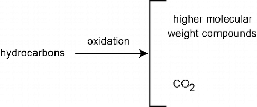
While the actual mechanisms of oxidation of the binder are elusive, it has been postulated that it is primarily oxidation of aromatics to form asphaltenes (Chavez-Valencia et al. 2007). An increase in molecular size with oxidation has been noted (Doh et al. 2008). Although not expected to occur to a large degree, complete oxidation of hydrocarbon molecules would produce carbon dioxide (CO₂), so CO₂ would be expected to evolve from asphalt when oxidation occurs, as shown in Figure 1.

Figure 1 CO₂ emissions from asphalt.

CO₂ is an important and well-known greenhouse gas. Although CO₂ actually has the lowest global warming potential (GWP, a scale of radiation capture potential of a gas given in units of CO₂ potential – i.e. CO₂ has a GWP of 1) of commonly measured greenhouse gases, we produce so much of it each year that its effect far outweighs that of other greenhouse gases (e.g. methane, N₂O, chloro-fluoro-carbons, etc.). In the past 150 years, the CO₂ level in the atmosphere has risen from 290 ppm to over 380 ppm (EPA 2007). Therefore, any improvement that can be made to the asphalt paving process to reduce CO₂ emission is worth research.

EAPA (2004) clearly shows that the bulk of the CO₂ emissions from asphalt pavements happen during the initial construction, because of the high temperature required for mixing and paving. Warm mix asphalt (WMA) additives such as Sasobit allow asphalt to reach the low viscosity needed for mixing and paving at a relatively lower temperature (Sasol 2006, FHWA 2008). Sasobit^®, a synthetic paraffin wax, melts around 99°C and reduces the viscosity of the asphalt binder. The addition of Sasobit allows the reduction of the production temperatures by 10–30°C. Thus, WMA has the potential for significantly lowering CO₂ and other emissions produced during the construction of asphalt pavements.

The use of WMA through the addition of Sasobit has the potential to reduce CO₂ emissions related to the asphalt pavement construction in two ways. A lower required temperature for mixing and paving will reduce oxidation of the asphalt binder thus reducing emissions. Additionally, a reduction of emissions will be realised in the form of saved energy, as lower construction temperatures will require the use of less energy which reduces CO₂ emissions when petrochemical energy sources are used.

Objective and scope of work

The objective of this research was to determine, using laboratory experimental methods and instrumentation, how CO₂ emissions from asphalt mixes created during the period between mixing and paving are affected by mixing/aging temperature, added asphalt content and Sasobit content. The scope of work consisted of the following:

•	evaluate the effect of temperature, added asphalt content and addition of the additive Sasobit on CO2 emissions from asphalt mixes;
•	investigate whether the addition of Sasobit affects asphalt absorption by aggregates and thereby changes the effective asphalt content; and
•	determine whether the additive Sasobit itself will have an effect on CO2 emissions.

Equipment, sample preparation and emission testing procedure

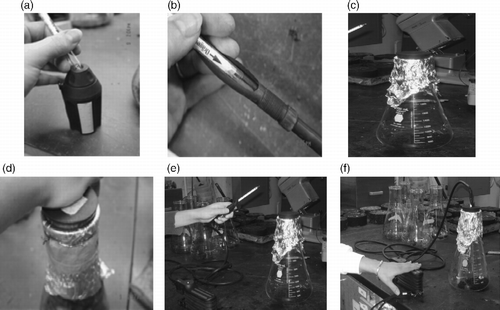
All CO₂ emissions were measured using an Accuro pump (Dräger Safety AG & Co., Luebeck, Germany, Dräger 2008) and 100–3000 ppm active flow CO₂ Dräger tubes. The pump was cleared with 10 strokes before each emission measurement was taken. The ends of each tube were removed using a Dräger tube opener, and the opened tube was inserted into the pump according to instructions. Ten pumps were used for each emission measurement as per the equipment instructions, and CO₂ concentration readings were taken at the end of the indicator discoloration to the nearest 50 ppm.

Samples were weighed and transferred to 2000 ml borosilicate glass Erlenmeyer flasks unless otherwise stated. The flasks were lightly agitated so that the sample was evenly distributed across the bottom. Aluminum foil was placed over the opening of the flask and wrapped with wire at the flask neck to give an airtight seal. All samples were cooled to room temperature before testing. A rubber stopper, with a hole for the Dräger tube, was placed over the top of the flask and pushed down through the foil seal. A second hole covered with a piece of masking tape containing a small pinhole prevented vacuum from forming in the flask during pumping. An open Dräger tube, already positioned in the pump, was immediately placed into the stopper hole and pumping was started to measure headspace CO₂ concentration. The equipment is shown in Figure 2.

Figure 2 Equipment and steps in testing: (a) the ends of each Dräger tube were removed using a tube opener, (b) the opened tube was inserted into the pump, (c) HMA mix samples were weighed and poured into 2000 ml borosilicate glass Erlenmeyer flasks, (d) a rubber stopper was placed over the top of the flask and pushed down through the foil seal, (e) an open Dräger tube, already positioned in the pump, was placed into the stopper hole and pumping was started and (f) 10 pumps were used for each emission measurement, and CO₂ concentration readings were taken at the end of the indicator discolouration to the nearest 50 ppm.

Testing plan and procedure

Effect of temperature, Sasobit content and asphalt content on CO₂ emission

Data for the CO₂ emissions model were collected at four different temperatures (110, 125, 155 and 175°C) for mixes with 1.5% Sasobit content and at three temperatures (125, 155 and 175°C) for mixes without Sasobit. At each temperature, 2–4 different added asphalt contents, ranging from 4 to 7% asphalt by weight, were considered. Based on the results of preliminary testings, three 200-g samples were taken at each combination of temperature, asphalt content and Sasobit content, and CO₂ emissions in the flask headspace were measured with Dräger testing equipment after 3 h of equilibrium time.

Effect of Sasobit on absorption of asphalt

Theoretical maximum density (TMD) tests were conducted to determine how the addition of Sasobit^® affects absorption of asphalt by the aggregate. TMD tests measure the greatest possible density an asphalt mix can have. Since the mass of aggregate, mass of asphalt and density of asphalt are constant for a given mix, the TMD value effectively indicates the effective specific gravity of aggregate (G _se). Because the density of unmixed aggregate, or bulk specific gravity of aggregate (G _sb), is also constant, the value of the G _se suggests how much of the aggregate's air void space has been filled with asphalt, or how much asphalt has been absorbed. For checking the effect of Sasobit on absorption through testing of theoretical maximum density (TMD, AASHTO T209) three 2000-g batches of aggregates where mixed with 5% asphalt content at 155°C for three different additions of Sasobit (0, 1.5 and 3%). The batches were heated for 2 h at mixing temperature and TMD tests were completed for all 12.

Effect of Sasobit on CO₂ emissions

A set of CO₂ emission tests were completed to see if Sasobit had any effect on the CO₂ emissions from asphalt containing the additive. Because Sasobit^® is itself a high carbon hydrocarbon, it was thought that perhaps the additive would alter the oxidation potential of asphalt.

Four 35-g samples of 155°C PG64-28 asphalt for each of the three different Sasobit additions, 0, 1.5 and 5%, were heated in sealed 600 ml beakers at 155°C for 3 h. The beakers were allowed to cool to room temperature after being removed from the oven, and CO₂ concentration measurements were taken using the Dräger equipment.

Materials

The asphalt/aggregate samples were first prepared in bulk by combining the constituents at mixing temperature (as close to the commercial asphalt/aggregate production process as possible), followed by the separation of the bulk material into individual samples that were transferred to the Erlenmeyer flasks for CO₂ emission tests as described above. This experimental procedure closely mimics the asphalt/aggregate production process, which is comprised of initial mixing, followed by transportation, idle time and placement. PG 64-28 asphalt obtained from Maine Department of Transportation (MDOT) was used for all experiments. The aggregates were obtained from a quarry in Westbrook, Maine that supplies aggregates to MDOT. All mixes were made with 1000 g of an aggregate mix consisting of 60% (600 g) stone (coarse aggregate, bulk specific gravity: 2.690 and absorption: 0.5%) and 40% (400 g) sand (fine aggregate, bulk specific gravity: 2.600 and absorption: 0.8%). The asphalt and aggregate were then mixed and spread in a pan to cool to room temperature. Once cooled the mixtures were separated into individual particles by hand, and then into coarse (stones) and fine (sand). From each mixture three 200-g samples comprising of 60% (120 g) coarse and 40% (80 g) fine sand were weighed and placed into the Erlenmeyer flasks. The flasks were sealed, placed in the oven at the temperature at which they were mixed and CO₂ emissions were measured in the flask headspace all according to the procedure outlined above.

Ambient laboratory CO₂ concentration

The ambient CO₂ concentration in the lab was also measured frequently to make sure it was not changing. After six consistent readings of 450 ppm over 6 days this was discontinued and 450 ppm was assumed to be the ambient CO₂ concentration (slightly higher than the reported standard atmospheric concentration of 380 ppm).

Results and analysis

CO₂ emission

The CO₂ emission data collected from experiments are summarised in Table 1. The ambient CO₂ concentration in the laboratory, determined to be 450 ppm, was subtracted from all CO₂ measurements taken. The resulting value represented CO₂ emissions created by the asphalt mixes.

Table 1 CO₂ emission data.

Asphalt content	Emission reading (ppm)	Net CO2 emissions = emission reading − ambient (ppm)	Average
No Sasobit
Temperature: 125°C
4%	650	200	233.3
	650	200
	750	300
5%	700	250	216.6
	600	150
	700	250
5.50%	650	200	250.0
	750	300
	700	250
6%	700	250	300.0
	800	350
	750	300
Temperature: 155°C
4%	1400	950	983.3
	1600	1150
	1300	850
5%	1500	1050	966.6
	1450	1000
	1300	850
5.50%	1400	950	1016.6
	1500	1050
	1500	1050
6%	1500	1050	1033.3
	1500	1050
	1450	1000
Temperature: 175°C
4%	2150	1700	1783.3
	2300	1850
	2250	1800
6%	2400	1950	1850
	2300	1850
	2200	1750
With Sasobit
Temperature: 110°C
4%	600	150	150.0
	650	200
	550	100
6%	650	200	166.6
	600	150
	600	150
Temperature: 125°C
4%	650	200	283.3
	800	350
	750	300
5%	800	350	316.6
	850	400
	650	200
6%	800	350	316.6
	850	400
	650	200
7%	800	350	416.7
	850	400
	950	500
Temperature: 155°C
4%	1350	900	966.6
	1450	1000
	1450	1000
5%	1500	1050	1033.3
	1650	1200
	1300	850
6%	1500	1050	1066.6
	1450	1000
	1600	1150
Temperature: 175°C
4%	2300	1850	1900.0
	2250	1800
	2500	2050
6%	2500	2050	1900.0
	2450	2000
	2100	1650

An analysis of variance (ANOVA) of the entire dataset was done with the null hypothesis that any of the standardised coefficients of the independent variables was zero. Rejecting this hypothesis would indicate that these independent variables show a relationship with CO₂ emissions even in the case that none of them showed a significant relationship individually.

Table 2 shows the results of the ANOVA for the regression model. This analysis confirms that at least one of the three independent variables, Sasobit^® content, temperature and added asphalt content, has a statistically significant effect on CO₂ emissions (Sig. < 0.000).

Table 2 ANOVA of linear regression model of CO₂ emissions with Sasobit^® content, temperature and added asphalt content.

	Sum of squares	d.f.	Mean square	F	Sig.
Regression	22,037,232.903	3	7,345,744.30	299.735	0.000
Residual	1,445,941.700	59	24,507.48
Total	23,483,174.603	62

A linear regression model analysis was done with CO₂ emissions as the dependent variable and Sasobit content, mixing/aging (heating) temperature and added asphalt content as the independent variables (SPSS 2008, statistical software was used). Individual t-tests on the relationships between emissions and each of the independent variables were also conducted. The t-test operated with a null hypothesis that the standardised coefficient (β) of each independent variable (i.e. the regression coefficient of the independent variable normalised by taking the Z score) is equal to zero. A non-zero β-value, assumed if the null hypothesis is rejected, would suggest that the two variables are related. The significance of this test is the probability that we will reject the null hypothesis when it is actually true (Type I error). The smaller this value is (the more significant the test is), the stronger the relationship between the two variables.

The results of the linear regression with CO₂ emissions as the dependent variable are shown in Table 3. Temperature is shown to have a very significant relationship (Sig. < 0.000) with CO₂ emissions. Sasobit^® content also seems to have a reasonably significant relationship (Sig. = 0.004) with CO₂. For this range of added asphalt contents (4–7%) there does not seem to be any strong correlation between asphalt content and emissions.

Table 3 Linear regression model of CO₂ emissions with Sasobit^® content, temperature and added asphalt content.

	Unstandardised coefficients		Standardised coefficients
Independent variable	B	Std. Error	β	t	Sig.
(Constant)	− 3341.569	183.917		− 18.169	0.000
Sasobit^® content	8119.577	2673.540	0.100	3.037	0.004
Temperature	27.693	0.927	0.984	29.880	0.000
Added asphalt	2529.813	2136.274	0.038	1.184	0.241

Revised CO₂ emission model

The results from this regression analysis prompted a second linear regression analysis including temperature as the only independent variable. Because temperature is likely the only meaningful significant factor in this model, the model was recreated ignoring the other independent variables. The results of ANOVA of this model are shown in Table 4a and the second linear regression in Table 4b. Both of these analyses show the relationship to be highly significant (Sig. < 0.000). A series of curve fits were also done to investigate potential nonlinear behaviour of this relationship and possibly a more accurate model for predicting CO₂ emissions. The parameters of these curve fits and their corresponding R ² values are shown in Table 4c.

Table 4a ANOVA of linear regression model of CO₂ emissions with temperature.

	Sum of squares	d.f.	Mean square	F	Sig.
Regression	21,771,556.26	1	21,771,556.265	775.912	0.000
Residual	1,711,618.33	61	28,059.317
Total	23,483,174.60	62

Table 4b Linear regression model of CO₂ emissions with temperature.

	Unstandardised coefficients		Standardised coefficients
	B	Std. Error	β	t	Sig.
(Constant)	− 3064.342	140.861		− 21.754	0.000
Temperature	27.111	0.973	0.963	27.855	0.000

Table 4c Curve fits for CO₂ emissions versus temperature.

	Model summary					Parameter estimates
Equation	R ^2	F	d.f.1	d.f.2	Sig.	Constant	b 1	b 2	b 3
Linear	0.927	775.91	1	61	0.000	− 3064.342	27.11
Quadratic	0.975	1187.87	2	60	0.000	4331.942	− 77.85	0.364
Cubic	0.976	1194.75	2	60	0.000	1891.856	− 25.91	0.000	0.001
Power	0.944	1021.80	1	61	0.000	6.45 × 10^− 10	5.55
Exponential	0.941	971.88	1	61	0.000	2.175	0.039

The highest R ²-value for a curve fit was for the cubic equation (R ² = 0.976). This does not necessarily indicate the true behaviour of the relationship as it would be hard to strongly conclude a cubic or quadratic relationship with the relatively small amount of collected data. One thing that is certainly clear from the data is that the relationship between temperature and emissions is something other than linear.

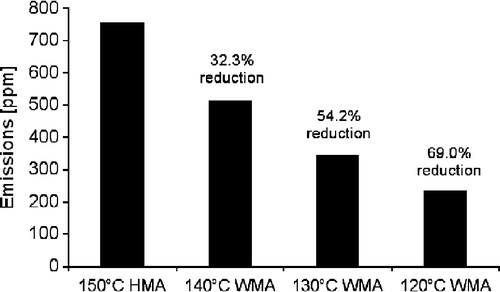
Using any one of the models, the reduction in emission due to a decrease in temperature can be estimated. For example, using the following exponential equation, the reduction in emission of CO₂ was estimated as shown in Table 5.

where is the CO₂ concentration in ppm expected in the 2000 ml flask headspace in equilibrium with 200 g of asphalt mixture and T is the mixing/aging temperature in degree Celsius.

Table 5 CO₂ reduction estimates for different temperature reductions.

HMA temperature (°C)	WMA temperature (°C)	HMA emissions (ppm)	WMA emissions (ppm)	% Reduction
150 (considering PG 64-28 asphalt binder)	140	755.23	511.3	32.29
	130	755.23	346.2	54.16
	120	755.23	234.4	68.96

The data are shown graphically in Figure 3.

Figure 3 Reduction in CO₂ emission with lower processing temperatures.

Additional CO₂ emissions reductions will occur as a result of less needed energy input.

The heat energy needed to increase the materials' temperature can be determined according to the following equation:

where Q is the energy needed for the temperature change, m is the mass of the material heated, c is the specific heat capacity of the material and ΔT is the temperature change.

If mixes of the same weight and composition are being compared, m and c are constant and ΔT can be used directly to quantify energy needed. Assuming that mixes are heated from room temperature (25°C), the energy savings from using WMA can be calculated as follows:

For the same temperature reductions considered in the previous section, the following CO₂ production due to reduced energy consumption would be realised (Table 6).

Table 6 Energy and CO₂ reduction estimates for reduced mix temperatures.

HMA temperature (°C)	WMA temperature (°C)	% Reduction
150	140	8
	130	16
	120	24

It can reasonably be assumed that CO₂ generated through petrochemical combustion for energy production is directly proportional to the mass of fuel burned. A reduction in energy needed to produce asphalt pavements would result from lower mix temperatures. Therefore, the percent savings in Table 6 are also representative of emission reductions for these temperature reductions.

The results from this study allow us to compare the percentage decrease in CO₂ emissions due to reduced oxidation of the asphalt mix because of lower mix temperatures needed with WMA. However, production and construction data could be used to calculate the actual savings in CO₂ emission due to a reduction in the amount of fuel that is needed for raising the temperature. Mix production data from Germany shows that a reduction of 10°C in the production temperature would lead to a reduction of 1.73 kg of CO₂ per metric tonne of mix produced (Butz 2008a). This number is based on the following data reported by Butz (2008a):

• Fuel needed for drying and heating 1 metric tonne of mix = 8 l.

• 1 l of fuel releases 2.7 kg of CO₂.

Therefore, for 8% reduction (from Table 6) in the amount of fuel required, the savings in the amount of CO₂ released = 1.73 kg (2.7 kg 0.08 8 l).

Note that in terms of actual number, this amount could be as significant as the reduction in CO₂ emitted from decreased oxidation of the mix.

The above data are based on light heating oil (boiling temperature range 180–360°C; average elemental composition C = 86.5%, H = 13.3%) and on dry aggregates (stored under roof). The plant is a typical batch mixing plant. It has been reported that the type of fuel as well as the plant configuration does not have a significant influence on the relative fuel and CO₂ savings if the burner is tuned for decreased mixing temperatures. However, the absolute fuel consumption and CO₂ release per tonne of hot mix depend on the individual plant configuration and the type of fuel used, e.g. in Europe some plants use natural gas (lower CO₂ emissions) or coal dust (higher CO₂ emissions; Butz 2008b).

Theoretical maximum density

The results from the 12 TMD tests, along with calculated absorptions are shown in Table 7. Note that absorption is calculated using the following equations:

where P _ba, absorbed asphalt (%); G _se, effective specific gravity of aggregate; G _sb, bulk specific gravity of aggregate; P _b, percent of asphalt binder in the mix and G _mm, theoretical maximum specific gravity (numerically equal to TMD in gm/cm³)

Table 7 TMD results (and calculated absorption) for different additions of Sasobit.

TMD (g/cm^3) (absorption, %)
Sample	No Sasobit^®	1.5% Sasobit^®	3% Sasobit^®
1	2.496 (1.5)	2.496 (1.5)	2.488 (1.3)
2	2.491 (1.4)	2.491 (1.4)	2.491 (1.4)
3	2.491 (1.4)	2.490 (1.4)	2.488 (1.3)
Average	2.493 (1.4)	2.492 (1.4)	2.489 (1.3)

A one-way ANOVA was conducted with the absorption data to see if changing Sasobit content caused a statistically significant change in absorption of the asphalt to aggregates. The results of this ANOVA (Table 8) show that these data do not support the hypothesis that there is a significant effect of the Sasobit content (Sig. = 0.125). This indicates that there is no relationship between the measured absorption and Sasobit content. This analysis suggests that Sasobit does not significantly affect absorption if the temperature remains constant.

Table 8 One-way ANOVA of absorption data with Sasobit^® content as an independent variable.

	Sum of squares	d.f.	Mean square	F	Sig.
Between groups	0.02	2	0.010	3.000	0.125
Within groups	0.02	6	0.003
Total	0.04	8

Effects of Sasobit on CO₂ emissions

The results of the analyses of Sasobit^® content effects on TMDs and CO₂ emissions provide little explanation as to why the addition of Sasobit^® seems to have a significant effect on emissions. Hence, the results from emission tests of asphalt (binder only) with and without Sasobit were examined more fully. The results of the CO₂ emission testing done with different percentages of Sasobit^® are listed in Table 9. Note again that the values listed in this table are the net CO₂ emissions (CO₂ readings minus background CO₂) and not the actual readings taken with the Dräger equipment.

Table 9 Net CO₂ emissions (ppm) for different additions of Sasobit^®.

Sample	No Sasobit^®	1.5% Sasobit^®	5% Sasobit^®
1	350	300	350
2	350	350	350
3	300	350	350
4	350	350	350
Note: The lack of difference between the three sets of numbers is apparent.

Table 10 contains the results of the one-way ANOVA of this data done with CO₂ emission as the dependent variable and Sasobit content as the independent.

Table 10 One-way ANOVA of Sasobit effects on emissions.

	Sum of squares	d.f.	Mean square	F	Sig.
Between groups	416.667	2	208.333	0.500	0.622
Within groups	3750.000	9	416.667
Total	4166.667	11

With a resulting significance of 0.622 it seems clear that the chemical properties of Sasobit itself do not change the oxidation potential of asphalt containing it. And it may be surmised that the Sasobit itself is not undergoing significant oxidative degradation, as it would have resulted in increased CO₂ production at greater Sasobit concentrations. Therefore, it is not directly responsible for any differences in CO₂ emission.

Conclusions and recommendations

Temperature seems to be the factor that most influences CO₂ emissions. Although the asphalt content of a pavement most likely does affect emissions, this effect is smaller than the sensitivity of the testing equipment for the range of asphalt contents used in the experimental setup. The added content range used in the experimentation is representative of that used in the practice, and therefore asphalt content can be assumed to have a negligible effect on CO₂ emissions in construction. This finding also suggests than any variation in effective asphalt content due to absorption can be neglected.

These results suggest that, considering the factors studied in this research, lowering the asphalt mix temperature is definitely the most effective way to reduce CO₂ emissions during asphalt mix production and pavement construction. The findings also support the use of the temperature lowering additives such as Sasobit to meet this end without seeming to cause any undesired effects on emissions or volumetric properties of the asphalt mix.

Today, WMA projects in the US typically use around 1.5% Sasobit^® in asphalt binder as this is currently the economically optimal value (Shaw 2008). A 1.5% Sasobit^® addition will generally allow for mixing and paving temperatures about 10–30°C (depending on the mix and project) lower than those for HMA. With these levels of Sasobit, CO₂ emission reductions of around 32% from direct reductions and another 8% reduction from energy savings is possible. This is an estimated joint reduction of about 40%. Although the reduction from burning less fuel is smaller in percentage, the actual numbers could be significantly higher than that from reduction of oxidation of the mix.

Continued attempts to lower asphalt construction temperatures should be undertaken as this is certainly the most effective way to reduce emission impact from this sector. However, emission reductions diminish with lower temperatures. Therefore, in the interest of lowering emissions, it may currently make more sense to focus efforts on implementing more widespread WMA projects than focusing on reducing temperatures further.

Acknowledgements

This material is based upon the work supported by the National Science Foundation under Grant No. 03-577 as well as in-kind contribution from MDOT. Any opinions, findings and conclusions or recommendations expressed in this material are those of the author(s) and do not necessarily reflect the views of the National Science Foundation and MDOT. The authors are deeply grateful to Thorsten Butz and John Shaw of Sasol Wax, and Mr Wade McClay and Mr Rick Bradbury of MDOT. The authors are also indebted to Margaret Pakula of Northwestern University, and Laura Rockett, Amy LeBlanc, Christine Keches, Mr Don Pellegrino and Mr Dean Daigneault of the Civil and Environmental Engineering Department at Worcester Polytechnic Institute (WPI).

Additional information

Notes on contributors

John Bergendahl

1 1 [email protected]

Notes

¹ [email protected]

References

- Butz, T., 2008a. Communication with, Sasol Wax GmbH, Hamburg, Germany, 25 July 08
- Butz, T., 2008b. Communication with, Sasol Wax GmbH, Hamburg, Germany, 17 November 08
- Chavez-Valencia , L.E. 2007 . Modeling the performance of asphalt pavement using response surface methodology – the kinetics of aging . Building and Environment , 42 : 933 – 939 .
- Doh , Y.S. , Amirkhanian , S.N. and Kim , K.W. 2008 . Analysis of unbalanced binder oxidation level in recycled asphalt mixture using GPC . Construction and Building Materials , 22 : 1253 – 1260 .
- Draeger, 2008. Available from: http://www.draeger.com/ST/internet/US/en/index.jsp [Accessed 16 July 2008]
- EAPA, 2004. Environmental impacts and fuel efficiency of road pavements. Prepared by Joint EAPA/Eurobitume Task Group Fuel Efficiency, March 2004
- EPA, 2007. ‘Greenhouse Gas Emissions.’ US Environmental Protection Agency. 16 April 2007. Available from: http://www.epa.gov/climatechange/emissions/index.html [Accessed 14 July 2007]
- FHWA, 2008. Warm mix asphalt technologies and research. US DOT FHWA. Available from: http://www.fhwa.dot.gov/pavement/asphalt/wma.cfm [Accessed 17 July 2008]
- Gasthauer , E. 2008 . Characterization of asphalt fume composition by GC/MS and effect of temperature . Fuel , 87 : 1428 – 1434 .
- Herrington , P.R. and Ball , G.F.A. 1996 . Temperature dependence of asphalt oxidation mechanism . Fuel , 75 ( 9 ) : 1129 – 1131 .
- Ouyang , C. 2006 . Improving the aging resistance of asphalt by addition of zinc dialkyldithiophosphate . Fuel , 85 : 1060 – 1066 .
- Sasol International, 2006. What is Sasobit®? Available from: http://www.sasolwax.com/Europe.html [Accessed 1 June 2006]
- Shaw, J., 2008. Presentation on Sasol at warm mix open house, Morro Bay, CA, May, 2008. Available from: http://www.warmmixasphalt.com/submissions/85_20080629_JohnShaw_Sosabit_Caltrans.pdf [Accessed 24 March 2009]
- SPSS, 2008. Available from: http://www.spss.com/ [Accessed 16 July 2008]
- Sutton, C.L., 2002. Hot blue smoke emissions. Technical Paper T-143, ASTEC, Chattanooga, TN, 2002
- Trumbore , D.C. 1999 . Estimates of air emissions from asphalt storage tanks and truck loading . Environmental Progress , 18 ( 4 ) : 250 – 259 .