Identifying and modeling key trade-offs between hydrogen fuel cell and electric vehicles

Abstract

Through a sensitivity analysis, the trade-off between vehicle range and CO₂ emissions is investigated as a function of electric emissions coefficient. Various powertrains were analysed for use in a small crossover sport utility vehicle. Gasoline, gasoline electric hybrid, diesel, fuel cell and battery electric vehicles (BEVs) were considered. Using various upstream fuel pathways and a model for vehicle performance, emissions and energy use were estimated. The hydrogen fuel cell vehicle was found preferable to BEVs under conditions of high CO₂ emissions per kW-hr and a high vehicle range requirement. The BEV was preferable for all other conditions.

Keywords:

• Fuel cell
• electric vehicle

1. Introduction

Advancements for cheaper, cleaner and more efficient power are leading to a wealth of different fuel and powertrain choices for advanced-technology vehicles. Policies directed at both powertrains and the energy grid will have an impact on which power platforms ultimately gain acceptance. For example, the environmental impact of any sort of plug-in vehicle is highly dependent on the source of electricity for the local grid. Therefore, it is essential to evaluate powertrains in a manner that allows a continuum of possibilities to be considered. Consumer choice will also play a role in which platforms are successful, so it is essential to compare vehicles that consumers would consider to be reasonable equivalents, if not identical, in terms of day-to-day operation and performance. From the consumer’s viewpoint, a fundamental difference between battery electric vehicles (BEV) and most other powertrains is that refuelling a BEV will take significantly longer than refilling a tank with gas or replacing a hydrogen tank. Electric vehicle range can be increased through additional batteries, but these batteries will reduce vehicle performance or increase the power required for the vehicle in order to maintain an equivalent acceleration. Therefore, the desired range of a BEV between recharging is an essential parameter in any comparison of alternative fuel powertrains.

While previous studies have addressed the performance of alternative fuel powertrains (Eaves and Eaves 2004; Liao, Weber, and Pfaff 2004; Mizsey and Newson 2001; Rousseau et al. 2003; Stodolsky et al. 1999), these investigations do have some drawbacks:

•	The electric grid’s mix sensitivity on the overall energy consumption and carbon emissions of advanced powertrains such as the BEV and hydrogen (via electrolysis) fuel cell is often overlooked.
•	Previous studies do not always ensure that vehicles compared are of equal mass-to-power ratio (i.e. acceleration performance).

While multiple speculative scenarios are often considered, possible grid CO₂ emission coefficient and consumer preference for vehicle range comparisons are usually treated as discrete variables, whereas they are truly continuous variables. A previous study (Maduro 2010) investigated overall energy consumption and carbon emissions for numerous powertrains as a function of grid electricity mix on a Toyota-Prius-sized vehicle. To reflect a vehicle more typical of the US market, this study simulates performance of various powertrains in small crossover SUVs of similar weight-to-power ratio while executing the US Federal Test Procedure-75 (FTP-75) drive cycle, also known as the city cycle. Results of this study are presented as a preference map that identifies regions of preference for one platform over another on a plot with desired vehicle range on one axis, and electric grid CO₂ emission coefficient on the other axis. A list of the powertrains and fuel pathways analysed is shown in Table 1. For the gasoline and diesel powertrains, fuel consumption numbers were obtained from manufacturer data. For the fuel cell vehicle (FCV), laboratory tests were used to establish input data for the simulations discussed. Lastly, for the BEV, a drive cycle model was utilized. For all six powertrains, an upstream emissions model was utilized.

Table 1. Powertrains analysed.

Fuel pathway	Powertrain
Gasoline (reformulated, 87 Octane number)	Spark Ignition Internal Combustion Engine – 2009 Ford Escape (SI ICE)
Gasoline (reformulated, 87 Octane number)	Spark Ignition Internal Combustion Engine/Hybrid – 2009 Ford Escape Hybrid (SI ICE/Hybrid)
Diesel (less than 15 ppm Sulfur, 42.5 min. Cetane number)	Compression Ignition Internal Combustion Engine – 2006 Jeep Liberty CRD (CI ICE)
H2 via natural gas reforming	Fuel cell electric vehicle (FCV/NGR)
H2 via national grid electrolysis	Fuel cell electric vehicle (FCV/E)
National grid electricity	Battery electric vehicle (BEV)

2. Simulation and baseline analysis

The simulation of vehicle emissions and energy usage was carried out in three distinct steps.

Well-to-tank (WTT) – Upstream emissions were estimated using Argonne National Laboratory’s Greenhouse Gases, Regulated Emissions and Energy Use in Transportation (GREET) Model (GREET Model 2013). This established the total upstream energy use as well as an emissions coefficient (i.e. grams CO₂ per unit of tank energy) for each fuel pathway.

Tank-to-wheel (TTW) – For conventional powertrains, existing manufacturer data were used to estimate fuel consumption of the vehicle while executing a drive cycle. For alternative powertrains (i.e. fuel cell and BEV), a powertrain model was developed in Matlab® to estimate tank energy consumption (either hydrogen or electricity). For the FCV, data for the powertrain simulation were obtained from experimental studies on a lab-scale hydrogen fuel cell.

Well-to-wheel (WTW) – The results of the WTT and TTW simulations were added to estimate overall energy usage and CO₂ emissions for each powertrain. An amortized CO₂ emission value was added to the BEV case to account for the manufacture of the battery.

Before discussion of specific simulation details, it is important to note both simulation and study limitations. First, excepting battery costs for the BEV, only WTW impacts were studied, not full manufacturing cycle cradle-to-grave impacts. The authors felt that the remaining life cycle costs for manufacturing would be comparable from platform-to-platform, and therefore would not have a great influence on platform-to-platform comparisons. Furthermore, only emissions and energy use were analysed. Costs of various powertrains were not considered and only a city drive profile (the FTP-75 cycle utilized for emissions and fuel economy characterization in the United States) was studied. The FTP-75 cycle is similar in nature to both the Japanese 10–15 mode as well as the new European drive cycle (NEDC) so similar results would be expected for analyses of these cycles. Although the US cycle is transient while the NEDC and Japan 10–15 are modal, all three incorporate idle stops, acceleration and braking events, and higher speed cruising. Furthermore, average cycle velocities, obtained using a 1-s running average of the velocity trace, are 34.1, 33.6 and 25.6 km/hr for the FTP-75, NEDC and Japanese 10–15 mode cycles, respectively. Thus, while exact emissions and energy usage results are cycle dependant, general trends are expected to be similar across all three major drive cycles. Lastly, auxiliary power draw for air conditioning and power steering systems while executing the FTP-75 drive cycle was not simulated.

2.1. WTT simulation

Five fuel pathways were analysed for upstream CO₂ emissions and energy consumption associated with production and distribution: conventional gasoline, ultra-low sulphur diesel, hydrogen via hydrocarbon reforming, hydrogen via electrolysis using grid electricity and grid electricity. For both gasoline and diesel, the current standard upstream production and refining methods were assumed. For hydrogen reforming, steam reforming of natural gas was assumed. For the grid-based electricity, a US national average fuel mix for upstream electric production was used for preliminary analyses, and then sensitivity analyses were performed.

For each pathway, Argonne National Lab’s Greenhouse Gases, Regulated Emissions, and Energy Use in Transportation (GREET) Model (version 1.8) was utilized (Wang, Wu, and Elgowainy 2005). Within GREET, a hypothetical vehicle can be analysed using fuels along a wide variety of pathways. The program outputs both total energy consumption and CO₂ emissions for the various user-specified fuel pathways. For the current study, the pathways outlined in Table 1 were chosen. These output totals from GREET are further broken into the three separate phases of energy use and emissions: feedstock, fuel and vehicle operations. Feedstock includes the recovery, transportation, storage and distribution of the feedstock used for fuel production. Fuel includes fuel production, transportation, storage and distribution. Vehicle operations encompass gaseous and particulate tailpipe emissions (i.e. exhaust emissions). By default, GREET assumes a vehicle of 10.14 L/100 km and makes certain assumptions regarding the gasoline equivalent fuel economy performance of various other alternative powertrains for scaling total vehicle operations energy use. However, in the current study, we used either actual manufacturer data or our own powertrain simulations for vehicle operation energy consumption rather than GREET’s. As such, the CO₂ output of GREET (for each phase) was divided by the GREET vehicle operations energy output for the various fuel pathways to determine an emissions coefficient (in terms of grams CO₂ per MJ of vehicle fuel tank energy). These coefficients are shown in Table 2. These emissions coefficients from GREET are now independent of our TTW simulation and efficiency assumptions. Coefficients (g/MJ), obtained from the GREET simulation, can then be multiplied by the vehicle’s TTW energy consumption (MJ/km) to determine the total CO₂ emissions per unit distance travelled (g/km).

Table 2. Calculated emissions coefficients.

Fuel pathway	CO2 emissions per unit tank energy (g/MJ)
	Feedstock	Fuel	Vehicle operations	Total
Gasoline	3.3	12.8	72.8	88.8
Diesel	4.8	9.9	74.9	89.6
H2 – reforming	5.3	99.1	0.0	104.4
H2 – electrolysis	305.2	0.0	0.0	305.2
Grid electricity	6.7	201.8	0.0	208.5

Likewise, for each fuel pathway, the GREET energy results for each of the three phases were divided by the vehicle operations phase to determine the amount of energy consumed in each phase per unit of tank energy. These coefficients are presented in Table 3. Like the CO₂ coefficients from Table 2, these can be multiplied by the vehicle’s energy consumption (from the TTW simulation described later) to determine the overall energy use.

Table 3. Calculated energy coefficients.

Fuel pathway	Energy use per unit tank energy (g/MJ)
	Feedstock	Fuel	Vehicle operations	Total
Gasoline	0.054	0.198	1.000	1.252
Diesel	0.054	0.141	1.000	1.194
H2 – reforming	0.078	0.664	1.000	1.742
H2 – electrolysis	1.393	1.463	1.000	3.856
Grid electricity (national average)	0.092	1.544	1.000	2.636

2.2. TTW simulation

As noted earlier, the coefficients from Tables 2 and 3 can be multiplied by the vehicle’s energy use, in say MJ/km, to determine WTW CO₂ emissions and energy use per km of travel. Since GREET does not accurately simulate the vehicle operations energy consumption for the alternative powertrain crossover SUV in questions, a different source of information was needed. For the first three of the six powertrains considered in Table 1, this was fairly straightforward. All three of these powertrains are linked to actual United States production crossover SUVs as noted in Table 1. Thus, the Environmental Protection Agency’s reported city fuel economy numbers for each of the gasoline vehicles (Fuel Economy Guide 2009) and the diesel vehicle (Fuel Economy Guide 2005) was used. It should be noted that outside the United States, the Jeep Liberty is available in the European Union, Egypt and Venezuela. The Ford Escape (sold as the Ford Maverick) is also available in the European Union, South Korea and other Asia/Pacific markets. Other similarly sized and powered gasoline and diesel utility vehicles are commercially available elsewhere worldwide. However, for both FCVs and the BEV, a simulation was needed to estimate vehicle fuel consumption while executing the FTP-75 city cycle. To simulate these three vehicles’ executing the FTP-75 drive cycle, a dynamic model was developed in Matlab®. Using vehicle parameters (mass, drag coefficient, rolling resistance coefficient, etc.) as well as the velocity and acceleration signals, the instantaneous rolling, aerodynamic, and acceleration loads can be calculated as well as power requirement. Integrating this signal with respect to time and dividing by overall distance travelled yields energy requirement per km.

For these simulations, a drag coefficient of 0.4, frontal area of 3.15 m², rolling resistance coefficient of 0.015 and empty-chassis mass (curb mass minus powertrain mass) of 1400 kg was assumed to model a small crossover SUV. To this empty-chassis mass, the mass of various powertrain components needed (electric motors, batteries, fuel cell, etc.) were added. Because vehicle energy consumption is highly sensitive to performance, care was taken to ensure all vehicles fell within a similar performance range. Although exact acceleration performance is influenced by vehicle aerodynamics, transmission design, tire selection, weight distribution, etc., it is a very strong function of mass-to-power ratio. Therefore, normalizing for this ratio ensures that all vehicles are in a comparable performance range. All three traditional vehicles considered herein fell between 12 and 15 kg/kW. Thus, for the three alternative fuel vehicles, powertrains were sized to achieve a mass-to-power ratio of 13.5 kg/kW. The authors feel this is an essential aspect to developing a useful study, as consumer preference is likely to be highly dependent on vehicle acceleration performance.

To model hydrogen FCV efficiency, experimental performance measurements were taken directly on a Ballard NEXA 1.5 kW fuel cell stack. Although not an automotive-sized fuel cell stack, it includes all the necessary balance-of-plant items, and provides a reasonable estimate of overall stack efficiency for scaling purposes. In addition, the Ballard stack was of reasonable cost for the study and is manufactured by a major fuel cell producer who also supplies automotive scale stacks. As noted, the stack includes all necessary balance-of-plant items such as an air compressor, water management system, etc. Performance characterization consisted of measuring the stack’s polarization (voltage vs. current) using a resistive load bank, peak power, efficiency and weight. Efficiency was calculated by measuring the hydrogen consumption and comparing its heating value to the gross power production. Peak gross stack efficiency (in terms of converting latent hydrogen to direct current (DC) electricity) was found to be 61.1%. Net stack efficiency, which subtracts the power needed to run all ancillary equipment, was 50.9%. These data were used to model a stack sufficient to meet the mass-to-power target of the study when implemented in a 1400-kg vehicle chassis. These efficiency numbers in converting hydrogen to electric power were then used in the dynamic vehicle simulation, outlined earlier, to estimate hydrogen consumption from the vehicle’s mechanical wheel energy requirement. In addition, 90% efficiency was assumed for the DC to alternative current (AC) power conversion system (Faria et al. 2013). Efficiency curves for electric-to-mechanical conversion in the electric motor were obtained by scaling up data on an Azure Dynamics model AC90 vehicle traction motor. Weight of the electric motor was also scaled up from data on the AC90. This resulted in a total FCV mass of 1707 kg.

For the BEV, a simulation similar to that as outlined above for the FCV was developed to obtain mechanical energy requirement at the wheels. Like the FCV, a powertrain efficiency estimate was needed to go from tank energy to mechanical wheel energy. The same AC90 vehicle traction motor as the FCV was utilized. Again, the motor was sized to meet the mass-to-power ratio target of 13.5 kg/kW. In addition, the mass of storage batteries to obtain a 550 km range was added. The battery pack was sized such that it would be completely discharged at the end of the vehicle’s range target. The effect of this assumption is addressed later in the paper. Lithium ion batteries of 540 kJ/kg (150 Wh/kg) power storage density were assumed. This resulted in an extremely heavy vehicle of 2550 kg mass. The impact of BEV range target on vehicle mass and efficiency will be discussed later in a sensitivity analysis.

The TTW energy consumption, or vehicle operations phase by GREET terminology, for each of the six powertrains is shown in Table 4. The conversion from the more conventional units of fuel use in the third column to MJ/km in the fourth simply involved the respective use of heating value and density for gasoline, diesel and hydrogen; and the energy content in a kW-hr of electricity. Note that EPA’s original data reports fuel economy for the gasoline and diesel vehicles in miles per gallon, but these were converted to appropriate SI units.

Table 4. Simulated TTW energy consumption.

Fuel pathway	Powertrain	TTW fuel use	TTW energy use, MJ/km
Gasoline	SI ICE	10.68 L/100 km	3.70
Gasoline	SI ICE/Hybrid	6.91 L/100 km	2.40
Diesel	CI ICE	10.68 L/100 km	4.13
H2 – reforming	FCV/NGR	0.962 kg/100 km	1.36
H2 – electrolysis	FCV/E	0.962 kg/100 km	1.36
Grid electricity	BEV	24 kW-hr/100 km	0.87

While some sense of intuition might exist for the fuel use of traditional gasoline or diesel vehicles, fuel use for the hydrogen fuel cell and BEV is somewhat counter intuitive. As a point of reference, Honda claims their FCX clarity achieves 96.5 km/kg of hydrogen (Honda FCX 2009), or 1.035 kg/100 km. This mileage is similar to the 0.962 kg/100 km predicted for the simulated fuel cell crossover SUV discussed in this study. Also, Tesla claims their Roadster electric vehicle achieves a combined EPA range of 354 km with an onboard storage capacity of 57 kW-hr of electricity (Tesla 2009). This yields a city fuel consumption of 16.1 kW-hr/100 km, as compared to our simulated electric vehicle’s city fuel consumption of 24.0 kW-hr/100 km. Furthermore, Tesla’s more recent Model S equipped with an 85 kW-hr pack yields and EPA-certified 426 km range, or approximately 19.9 kW-hr/100 km. Results for both the fuel cell and BEV simulations performed here seem reasonable when compared to results for actual alternative fuelled vehicles, especially considering the weight penalty our vehicle has due its long range and utility nature (2550 kg) verses the lightweight roadster-based Tesla (1250 kg) with more energy-dense (and expensive) batteries.

2.3. WTW simulation

With the coefficients in Tables 2 and 3, as well as the vehicle energy use in Table 4, the overall WTW CO₂ emissions and energy consumption can be calculated by multiplying the two. Results for energy consumption are presented in Table 5 and Figure 1. Results for CO₂ emissions are presented in Table 6 and Figure 2. Results are broken down by the three GREET-defined phases of WTW energy use and emissions.

Table 5. Simulated well-to-wheel results for energy consumption.

Powertrain	Energy consumption (MJ/km)
	Feedstock	Fuel	Vehicle ops	Total
SI ICE	0.20	0.73	3.70	4.64
SI ICE/Hybrid	0.13	0.47	2.40	3.00
CI ICE	0.22	0.58	4.13	4.94
FCV/NGR	0.11	0.90	1.36	2.37
FCV/E	1.89	1.99	1.36	5.24
BEV	0.08	1.34	0.87	2.28

Figure 1. Well-to-wheel energy use comparison.

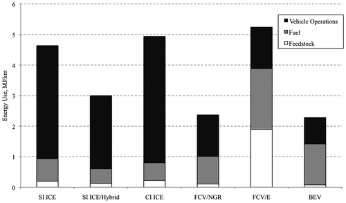
Table 6. Simulated well-to-wheel results for CO₂ emissions.

Powertrain	CO2 emissions (g/km)
	Feedstock	Fuel	Vehicle ops	Total
SI ICE	12.06	47.51	269.49	329.06
SI ICE/Hybrid	7.80	30.74	174.37	212.92
CI ICE	19.95	40.84	309.64	370.43
FCV/NGR	7.18	134.71	0.00	141.90
FCV/E	414.91	0.00	0.00	414.91
BEV	5.80	174.70	0.00	180.51

Figure 2. Well-to-wheel CO₂ emissions comparison.

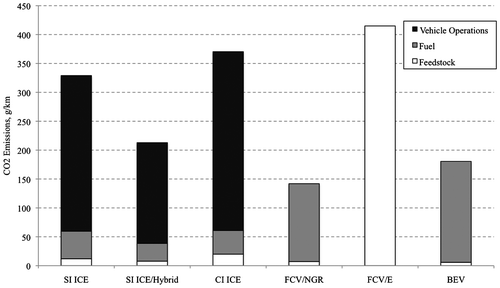
As shown, the first three conventional liquid hydrocarbon-fuelled vehicles have a small upstream energy requirement for petroleum drilling and refining, and thus low carbon footprint during these stages. However, the majority of the energy use and carbon emissions take place during vehicle operations due to the inefficiency of the internal combustion process. Of the three conventional powertrains, the spark ignition gasoline hybrid vehicle had the lowest energy use and CO₂ emissions. For the three alternative powertrains, much less energy is used during vehicle operations due to the highly efficient fuel cell and electric powertrains. However, significant energy is needed upstream for either hydrogen or electric generation. These three vehicles have zero tailpipe CO₂ emissions, but are not free from upstream CO₂ release. Overall, the lowest energy consumption was achieved by the BEV at 2.28 MJ/km with the FCV with natural gas reforming (NGR) closely trailing at 2.37 MJ/km. From a carbon footprint standpoint, the FCV/NGR have the lowest with only 141.9 g/km with the BEV a close second at 180.51 g/km. These results are similar to those reported by earlier researchers (Rousseau et al. 2003) in their WTW study of a full-size 2002 Ford Explorer SUV with various alternative powertrains. In that study, four fuel cell powertrains, all utilizing natural gas-sourced hydrogen but differing in onboard storage technique and powertrain layout, achieved emissions at or near 124.3 g/km. Furthermore, all four of the fuel cell powertrains simulated achieved WTW energy consumptions at or near 2.17 MJ/km. Both the WTW energy and CO₂ emissions figures for the cited study agree very well with the FCV/NGR vehicle simulated in the current investigation. Overall, small differences in energy usage and CO₂ emissions between the previous study and the current investigation are expected, given the fact that two are looking at vehicles of different type, mass and aerodynamics (i.e. full size SUVs in Rousseau et al. (2003), study vs. crossover SUVs in the current investigation).

It is interesting to note the high energy consumption and emissions from the electrolysis-based hydrogen FCV as compared to directly reforming natural gas. This is due to both the inefficiency of the electrolysis process, as well as the relatively dirty nature of the current average of US grid electricity. It should be noted that for the FCV with electrolysis (FCV/E), all of the CO₂ emissions are associated with feedstock production (in this case electricity) since the production of the vehicle’s fuel (hydrogen) from the feedstock and vehicle tailpipe emissions are both CO₂ free. This is illustrated in Figure 2.

3. Sensitivity of results to grid electricity emissions and vehicle range targets

In terms of sensitivity to input parameters, changes in vehicle specifications such as mass, drag coefficient, frontal area and rolling resistance coefficient would help or hurt all powertrains equally. For the current study, vehicle parameters were chosen to match those of the production gasoline and diesel vehicles compared against. In addition, changes in drive cycle between the FTP-75 and NEDC are not expected to fundamentally change the outcomes since both cycles are close in average velocity. However, there is an input parameter that does cause large changes in the results. For both the electrolysis-sourced hydrogen FCV and the BEV, WTW energy and emissions are highly dependent on where the electricity comes from. Increasingly, state legislations are pushing the grid in the direction of cleaner electricity. Thus, a sensitivity analysis was carried out to determine the total WTW CO₂ emission from these two vehicles across a range of possible electric grid conditions.

Figure 3 shows the sensitivity of the WTW emissions with respect to the cleanliness, in terms of grams CO₂ per kW-hr, of supplied grid electricity. Flat lines for the conventional Spark Ignition Internal Combustion Engine (SI ICE) vehicle and SI ICE/Hybrid are shown as references. These are flat since their emissions are not dependent on grid electricity. For the FCV, instead of plotting two separate lines for the electrolysis and NGR FCV, a single ‘best case emissions’ line is shown. At zero specific grid emissions, the ‘best case’ FCV is the electrolysis-sourced hydrogen. The CO₂ emissions then increase as the electric source becomes dirtier. Eventually, the line kinks flat (at approximately 256 g CO₂ per kW-hr) at the emissions level of a FCV/NGR since such a car would make sense over the electrolysis-based vehicle for all cases with higher values of CO₂ per kW-hr. For the BEV, WTW emissions are also a function of specific grid emissions. However, WTW emissions for the BEV are also a strong function of vehicle range. This is because increased range requirements result in a much heavier car, which in turn requires more energy to complete the FTP-75 cycle and maintain mass-to-power ratio. For the analyses discussed in this section, a span of possible BEV ranges from 0 to 1000 km is considered, which encompasses everything from only neighbourhood range all the way up to more ranges than a typical person could traverse in a single day before driver exhaustion.

Figure 3. CO₂ emissions as a function of grid emissions.

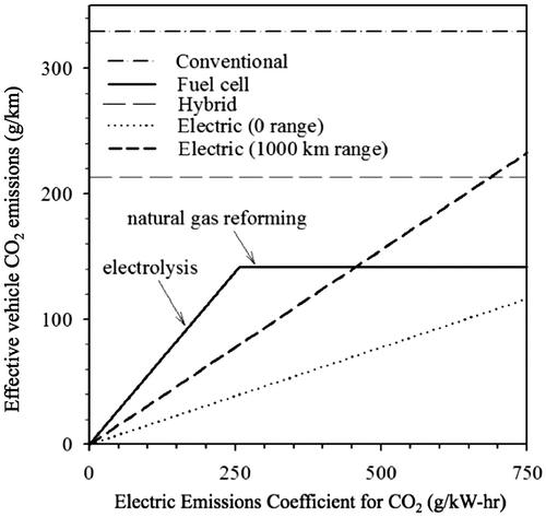
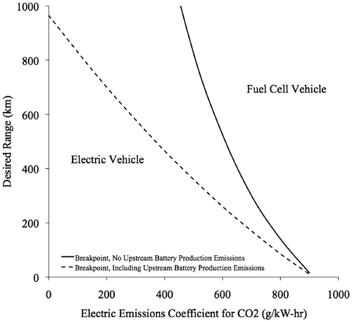
From a WTW CO₂ standpoint, the decision between a FCV and a BEV is dependent not only on how clean the grid is, but also on the range requirements for the electric vehicle. For the FCV, range is not as much of a concern, since hydrogen can be refuelled quickly. As the grid becomes cleaner, and moves leftward on the grid emissions axis of Figure 3 to less than approximately 450 g CO₂ per kW-hr, the case for BEV over an FCV becomes strong regardless of BEV range requirements. Based on these results, a preference map between the BEV and FCV was developed. This preference map (Figure 4) shows the optimal breakpoint, from a CO₂ perspective, between the BEV and FCV, as a function of grid emission coefficient and range requirement. The solid line refers to this optimal breakpoint based on CO₂ per km, whereas the dashed line accounts for battery upstream production emissions.

Figure 4. BEV and FCV breakpoint as a function of grid emissions and BEV range requirement.

While the current study does include the upstream WTT emissions associated with fuel production and distribution, no attempt was made to compare the upstream emissions associated with vehicle manufacturing and production. Because the various powertrains simulated vary greatly in terms of mechanical components and raw materials required, such a study would justify a separate investigation. However, an attempt was made to quantify the effect of battery production alone on the energy consumption and CO₂ emissions per km. To do this, the production energy and CO₂ emissions were amortized over an estimated 250,000 km vehicle life. As shown in Tables 5 and 6 and Figures 1 and 2, the BEV consumed 2.28 MJ and emitted approximately 180 g of CO₂ per km travelled. As noted, this does not include battery production. In their life cycle assessment of plug-in hybrid vehicles, Samaras and Meisterling (2008) used the energy estimates of Rydh and Sandén (2005) to arrive at 1700 MJ of energy consumed and 120 kg of CO₂ equivalent greenhouse gases emitted per kW-hr of Lithium-Ion battery storage capacity produced. For the base BEV case of 550 km range, our simulations predicted a 132 kW-hr pack needed. Using the aforementioned estimate of energy consumed in battery production and estimated vehicle life, this results in 224,400 MJ of energy required. Amortized over the life of the vehicle results in energy consumption increasing from 2.28 to 3.18 MJ/km travelled. Doing the same for CO₂ results in an increase to 244 g/km travelled.

In a similar fashion to before, the sensitivity of this newly calculated CO₂ emission level per km travelled was then analysed with respect to changes in desired electric vehicle range and specific grid electric emissions. As illustrated by the dashed line in Figure 4, the optimal breakpoint has shifted significantly. It must be stressed again that only battery upstream production emissions were analysed here, and no attempt was made to quantify the upstream emissions associated with fuel cell production. However, the above analysis illustrates the strong effect upstream production efficiency can have on optimal vehicle choice.

As shown, the BEV is preferential to the FCV in most cases except for those areas with high grid electricity emission coefficient and large vehicle daily range requirement. To illustrate the usefulness of Figures 3 and 4, consider two regions of the United States with very different electricity sources. In California, the average grid emissions are 277 g of CO₂ per kW-hr (Updated State-Level 2002). The BEV is preferential to both FCV powertrains even at an electric storage range requirement as high as 1000 km for this grid emission coefficient. However, in West Virginia, average grid emissions are 899 g of CO₂ per kW-hr (Updated State-Level 2002). The FCV is preferential for all but the smallest range requirements for this grid emission coefficient.

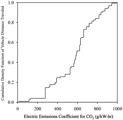
State-by-state vehicle miles travelled (VMT) data (Highway Statistics 2007) were obtained for all 50 states in the United States, and sorted from lowest to highest in terms of each state’s specific electric grid emissions (Updated State-Level 2002). Low-specific-emissions states include those with large nuclear and hydroelectric sources, while high-specific-emissions states are those almost entirely dependent on coal combustion. This VMT data were then integrated to obtain a cumulative density function and plotted verses specific grid emissions, as shown in Figure 5. Thus, cumulative density of unity corresponds to the total VMT in 2007 in the United States, which was 4.9 × 10¹² km. Combining this information with that from Figure 4 paints an interesting picture. For example, with today’s current grid, only a small portion of all distances travelled occur in areas where the grid is so dirty (> 900 g CO₂ per kW-hr) that an FCV always makes sense over the BEV regardless of range requirement. From Figure 5, approximately 80% of all distances travelled occur in areas of less than 800 g CO₂ per kW-hr electricity. Using that and referring back to Figure 4, a BEV with approximately 150 km range would be advantageous over the FCV for 80% of all distances travelled in the United States, ignoring upstream battery production emissions. Including these, a BEV with approximately 100 km range would be advantageous over the FCV for 80% of all distances travelled.

Figure 5. Cumulative fraction of vehicle distance travelled as a function of specific electric grid emissions coefficient.

4. Conclusion

Six powertrains were modelled to determine WTW energy consumption and CO₂ emissions in a crossover SUV using a combination of upstream fuel pathway emissions estimation software, EPA vehicle data, manufacture data on alternative vehicle powertrain components, in-lab experimental testing on a fuel cell stack and original vehicle powertrain simulations while executing the FTP-75 city cycle. The three conventional powertrains included a gasoline, gasoline electric and diesel. The three alternative powertrains included a BEV and two hydrogen FCVs (one with electrolysis and the other with NGR-based hydrogen generation). Of the six powertrains analysed, from an energy and carbon-footprint standpoint, the NGR-sourced hydrogen FCV and the BEV showed the greatest improvement over traditional technologies. Overall, the lowest energy consumption was achieved by the BEV at 2.28 MJ/km with the FCV with NGR closely trailing at 2.37 MJ/km. From a carbon footprint standpoint, the FCV/NGR have the lowest with only 141.9 g/km with the BEV a close second at 180.51 g/km. As noted earlier, these results are similar to those reported by earlier researchers (Rousseau et al. 2003) in their WTW study of a full-size 2002 Ford Explorer SUV with various alternative powertrains. In that study, all four fuel cell powertrains achieved emissions at or near 124.3 g/km and WTW energy consumptions at or near 2.17 MJ/km.

The optimal choice between the FCV and BEV vehicles is dependent on both the specific grid CO₂ emissions in a region and the vehicle daily range requirements for the electric vehicle. A preference map was developed to graphically illustrate the effect of these two parameters in making a battery vs. FCV decision. For example, the Tesla Model S 426 km range represents the high end of BEV ranges available on the market today. For the small crossover SUV modelled in this paper, the preference line between BEV and HFC vehicles for a 426 km range occurs at a local grid emissions coefficient of approximately 410 g/kW-hr when life cycle costs of battery production are accounted for. This grid coefficient in turn corresponds to the cleanest 25% of the US electric grid weighted for VMT. Note that the shape of the preference map for a sedan such as the Tesla Model S will be different from the preference map developed herein. The preference line for the 50 and 75% of the weighted electric grid emission coefficients correspond to vehicle ranges of approximately 225 and 175 km, respectively.

The preference map can also be viewed as a sensitivity study for two highly uncertain variables. The greenhouse gas emissions for the electric grid in the future will be highly dependent on the result of public policy and technological advances. Likewise, consumer preference for vehicle range under widespread alternative powertrain vehicle adoption is difficult to predict. Driving behaviours and requirements for early adopters of alternative powertrain vehicles might not reflect the behaviours and requirements of the population at large. While early entries to the BEV market will likely have fixed battery pack sizes, and therefore vehicle range, later entries might allow for more consumer choice, or perhaps the options will be adjusted to meet consumer preference.

This analysis showed that for most combinations of reasonable commuter-range requirement and grid cleanliness, a BEV is preferred over the FCV. For longer range requirements in regions with less-clean electric grid, the hydrogen FCV becomes preferable. The exact grid cleanliness and range requirement breakpoint between the battery or FCV is dependent on upstream production efficiencies for the battery pack, and accounting for life cycle costs of battery production shifts the preference life significantly for longer vehicle ranges.

Acronyms
BEV	=	battery electric vehicle
CI	=	compression ignition
E	=	electrolysis
EPA	=	Environmental Protection Agency
FCV	=	fuel cell vehicle
FTP	=	Federal Test Procedure
GREET	=	Greenhouse Gases, Regulated Emissions, and Energy Use in Transportation
ICE	=	Internal Combustion Engine
NEDC	=	new European drive cycle
NGR	=	natural gas reforming
SI	=	spark ignition
SUV	=	sport utility vehicle
TTW	=	tank to wheel
VMT	=	vehicle miles traveled
WTT	=	well to tank
WTW	=	well to wheel

Acknowledgements

The authors would like to acknowledge Mr James G. Kostic for his contributions towards developing the fuel cell experimental apparatus and obtaining performance data.

Disclosure statement

No potential conflict of interest was reported by the authors.

References

- Eaves, S., and J. Eaves. 2004. “A Cost Comparison of Fuel-cell and Battery Electric Vehicles.” Journal of Power Sources 130 (1–2): 208–212.10.1016/j.jpowsour.2003.12.016
- Faria, R., P. Marques, P. Moura, F. Freire, J. Delgado, and A. de Almeida. 2013. “Impact of the Electricity Mix and Use Profile in the Life-cycle Assessment of Electric Vehicles.” Renewable and Sustainable Energy Reviews 24: 271–287.10.1016/j.rser.2013.03.063
- Fuel Economy Guide (DOE/EE-0302). 2005. U.S. Department of Energy Office of Energy Efficiency and Renewable Energy.
- Fuel Economy Guide (DOE/EE-0325). 2009. U.S. Department of Energy Office of Energy Efficiency and Renewable Energy.
- GREET Model. 2013. U.S. Department of Energy Transportation and Technology R&D Center, Argonne National Laboratory.
- Highway Statistics. Table VM-2. 2007. U.S. Department of Transportation Federal Highway Administration.
- Honda FCX Clarity Fuel Cell Vehicle Specifications. American Honda Motor Corporation. Accessed November 2015. http://automobiles.honda.com/fcx-clarity/specifications.aspx
- Liao, G., T. Weber, and D. Pfaff. 2004. “Modelling and Analysis of Powertrain Hybridization on All-wheel-drive Sport Utility Vehicles” Proceedings of the Institution of Mechanical Engineers – Part D – Journal of Automobile Engineering 218 (10): 1125–1134.10.1177/095440700421801007
- Maduro, M. 2010. “Well-to-wheel Energy Use and Greenhouse Gas Emissions Analysis of Hypothetical Fleet of Electrified Vehicles in Canada and the U.S.” Masters diss., University of Ontario Institute of Technology.
- Mizsey, P., and E. Newson. 2001. “Comparison of Different Vehicle Power Trains.” Journal of Power Sources 102 (1–2): 205–209.10.1016/S0378-7753(01)00802-3
- Rousseau, A., R. Ahluwahila, B. Deveille, and Q. Zhang. 2003. “Well-to-wheels Analysis of Advanced SUV Fuel Cell Vehicles.” Society of Automotive Engineers 2003-01-0415.
- Rydh, C., and B. Sandén. 2005. “Energy Analysis of Batteries in Photovoltaic Systems. Part I: Performance and Energy Requirements.” Energy Conversion and Management 46: 1957–1979.10.1016/j.enconman.2004.10.003
- Samaras, C., and K. Meisterling. 2008. “Life Cycle Assessment of Greenhouse Gas Emissions from Plug-in Hybrid Vehicles: Implications for Policy.” Environmental Science and Technology 42: 3170–3176.10.1021/es702178s
- Stodolsky, F., L. Gaines, C. Marshall, and F. An. 1999. “Total Fuel Cycle Impacts of Advanced Vehicles.” Society of Automotive Engineers 1999-01-0322.
- Tesla Roadster Specifications. Tesla Motors Incorporated. Accessed August 2009. http://www.teslamotors.com/performance/perf_specs.php
- Updated State-level Greenhouse Gas Emission Coefficients for Electricity Generation 1998–2000. 2002. U.S. Department of Energy – Energy Information Administration.
- Wang, M., Y. Wu, and A. Elgowainy. 2005. The Greenhouse Gases, Regulated Emissions, and Energy Use in Transportation (GREET) Model, Operating Manual for GREET, Version 1.7 (ANL/ESD/05-3). Argonne National Lab.