Optimizing a two-echelon serial supply chain with different carbon policies

Abstract

In recent years, organizations are becoming environment conscious due to stringent laws, competitive advantages and increasing awareness of customers. They are integrating environmental practices into their operations to curb carbon emissions. Regulatory bodies are also imposing carbon policies to check emission. In this paper, we developed three models considering three carbon policies (I. carbon tax, II. strict cap and III. cap-and-trade) and have determined the optimal order quantity and number of shipments for a two-echelon supply chain. The objective is to minimize the total supply chain cost which comprises the ordering, setup, production, inventory holding and transportation costs. In Model I tax on carbon emissions has been included in the cost function; in Model II we have considered a strict carbon cap on the total carbon emission; and in Model III trading price of carbon is included in the cost function. A numerical study is given to illustrate the solution procedure. Further, sensitivity analyses are performed to examine the impact of the various parameters on the total cost and total emission.

Keywords:

• Carbon tax policy
• strict cap policy
• cap-and-trade policy
• vendor–buyer model

1. Introduction

Environment pollution is a burning issue in recent time. Continuous emissions of greenhouse gases into the atmosphere due to rapid industrial progression have raised the threat to environment and existence of human civilization. Scientists have revealed that over the past 130 years the average temperature of the earth has raised by approximately 0.85 °C. It is anticipated that between 2030 and 2050 approximately 250,000 deaths will take place annually due to weather change. Melting glaciers, rising sea levels, extreme weather conditions are result of global warming (WHO 2015). To address these issues organizations pay a great deal of attention for reducing greenhouse gases, associated with industrial operations. In recent years, organizations are paying emphasis on green and sustainable operations for different socio-economic reasons, such as government regulations, financial benefits, competitive advantage, ISO certification, customer satisfaction (Giunipero, Hooker, and Denslow 2012).

The view that human activities are responsible for increase in global temperature and environmental pollution has driven governments and different regulatory bodies to take initiatives and set realistic targets to curb emission. The Kyoto protocol, a part of the United Nations Framework Convention on Climate Change, targeted to reduce emission by 8% from 1990 levels by 2012. Scientists have suggested more aggressive target reduction of 25% from 1990 level by 2020 (Kinaxis 2009). To materialize this target regulatory bodies have imposed several laws and initiated different carbon policies. The existing carbon policies can be classified under three basic categories: carbon cost/tax policy, carbon cap-and-trade policy and strict carbon cap policy. Among these policies, carbon taxes and carbon markets (carbon cap-and-trade) are recognized as the most cost-effective mechanisms (Labatt and White 2007). The biggest international scheme for trading of greenhouse gases (GHG) is European Union Emissions Trading Systems (EU-ETS), which follows cap-and-trade concept, in which companies get an upper limit on green house gas emission and beyond this limit companies get penalized. If companies emit less than the specified limit, they can sell it off or keep as unused allowance (Jaber et al. 2013). If regulatory bodies reduce the limit of emission level, carbon price in the market goes up. Hence, the firms that manage its emissions well can only sustain in the market under cap-and-trade policy (Abhishek, Nidhi, and Pillai 2012). On the other hand, the United States has imposed a revenue neutral carbon tax policy, where every unit of carbon dioxide is chargeable (Metcalf 2009). In India, the Environment Ministry introduced a market-friendly pollution control system to encourage industries to reduce emissions. It was a two-year pilot trading scheme, covered 1000 industries of Gujrat, Tamil Nadu and Maharashtra. It puts a price for emissions, which makes polluting activities costlier and discourage industries to pollute (ET Bureau 2011). All these schemes are developed based on either carbon tax or carbon cap model. It has been observed that emission quantity restrictions are suitable when incremental damages increase drastically with the level of emissions or when marginal costs are relatively flat. In this case, quantity restrictions prevent emissions from rising above a desired level (Morgenstern 2002).

Initially, all the environmental initiatives were organization centric. But in constantly changing business world, companies cannot compete solely as individual entities. Nowadays, all the big business houses are part of one or more supply chains (SCs). It has been observed that 50% of the industrial-added values are derived from SC (Ciliberti, Pontrandolfo, and Scozzi 2008). SC has enhanced efficiency, improved productivity, reduced waste and squeezed capital investment (Carbon Trust 2006) and today profit is not only the concerned area, stakeholders are getting concerned about sustainability also (Dekker, Bloemhof, and Mallidis 2012).With the increasing environmental awareness in public and the implementation of new regulations in some countries, there is increased pressure on organizations to improve environmental performance. So, incorporation of environmental aspects into SC has become call of hours. Integration of environmental thinking into supply chain management (SCM) including product design, material sourcing, manufacturing processes, delivery of the product to the customers and end-of-life management of the product after its use can be defined as green supply chain management (GSCM) (Srivastava 2007). Sustainable supply chain management (SSCM) is another coeval concept exists in the area of SCM to deal with environmental issues. SSCM pay emphasis on economic, ecological and social issues (Svensson 2007).

2. Literature review

Environment pollution due to carbon emission is a major concern in recent times among the industries and research community. As a result of deteriorating environment and government regulations the concepts of GSCM and SSCM have gained momentum in both industry and academia. Both GSCM and SSCM have helped to reduce the environmental impacts of industrial activity. Apart from environmental reasons and regulations, studies have revealed that profitability and economic sustainability are also some of the main motivators for business organizations to adopt SSCM and GSCM (Srivastava and Srivastava 2006; Srivastava 2007; Svensson 2007; Darnall, Jolley, and Handfield 2008). The first concept of GSCM was brought into literature way back in 1989 by Kelle and Silver (1989). Mitra and Datta (2013) mentioned that discussions on GSCM have not gained momentum until early 2000. In the last couple of years, some papers have discussed about different aspects of GSCM and SSCM and enriched the existing literature. But the number of literature on GSCM is still limited (Dheeraj and Vishal 2012). We present a brief overview of recent work carried out in the area of SSCM and GSCM.

Svensson (2007) described and depicted different aspects of SSCM. He introduced the terms like first-order, second-order and n-order supply chains while discussing corporate effort in SSCM and provided an empirical study on clothing industry to explain the conceptual framework. Seuring and Müller (2008) introduced a wide spectrum of literature review comprising as many as 191 papers published from 1994 to 2007 in the area of SSCM. They provided a framework to summarize and categorized the existing literature. They observed that the papers pertaining to SSCM can be classified under three basic categories based on the area they dealt with. They found the papers have considered any of the three following areas: (i) environmental issues, (ii) social issues, (iii) both the issues. Authors also categorized papers, they reviewed on the basis of research methodology under the following categories: (i) papers dealt with theory and concept, (ii) case studies, (iii) surveys, (iv) papers with modelling and (v) literature review. Carter and Rogers (2008) discussed how loosely the term “sustainability” is defined and discussed in the literature. They presented a framework to integrate and extend different perceptions about sustainable supply chain and provided a holistic view about it. Pagell and Wu (2009) focused on the unique practices, adopted by the sustainable organizations. They revealed that alignment of financial and environmental goals are the bottom lines to attain sustainability. Gold, Seuring, and Beske (2010) discussed how organizations follow sustainable practices across the SC to gain competitive advantages. They also focused on interlinking of SSCM, strategic management and social network. Carter et al. (2011) presented an extensive review work considering empirical papers published in the area SSCM spanning over almost 20 years (1991–2011). All the aforementioned papers have dealt with either literature review or empirical study. In this paper, we have formulated mathematical models while dealing with environmental issues. In recent years several authors have developed mathematical models to handle environmental issues while considering different carbon policies in SC, but the number of such papers is still scant. In the following section, we discuss about some of these papers which have developed mathematical framework while considering different carbon policies for different production-inventory models and supply chains.

Dobos (2005) introduced tradable permits of carbon in the production-inventory strategy of a firm while extending basic Arrow–Karlin model (a well-known dynamic production-inventory model). Later, Dobos (2007) extended his earlier work with time-dependent price of unit tradable permit. Ramudhin et al. (2008) developed a mixed-integer mathematical model taking carbon trading into consideration within the SC network design phase. Diabat and Simchi-Levi (2009) formulated a mixed-integer program to determine an optimal strategy for companies to minimize cost considering carbon cap. Chen et al. (2010) developed a two-stage inexact stochastic programming method for planning carbon dioxide emission trading under uncertainty. Managing carbon emissions in inventory handling under the carbon emission trading policy has been discussed by Hua, Cheng, and Wang (2011). Bouchery et al. (2012) redesigned the classical EOQ model taking sustainability criteria into account under carbon cap and carbon price mechanism. Hoen et al. (2012) investigated the effect of different types of regulations with respect to emissions on the selected transport mode and the corresponding emissions. An optimization model for green SC was developed by Abdallah, Diabat, and Simchi-Levi (2010) to determine lot size for production and shipment for raw materials and finished products taking carbon emission constraints into consideration. Absi et al. (2012) developed multi-sourcing lot-sizing problems with periodic, cumulative, global and rolling carbon emission constraints. Jaber et al. (2013) developed a model to determine the optimal manufacturer’s production rate and vendor–buyer coordination multiplier, while considering carbon tax, emission penalty, emission allowance trading and combination of carbon tax and emission penalty. Benjaafar, Li, and Daskin (2013) considered carbon tax, strict emission cap, cap-and-trade, carbon offset while determining the optimal production, inventory, backorder quantity and amount of carbon traded to minimize the total supply chain cost for a single firm and they also extended their models for multiple firms with or without coordination in multi-period setting. Fahimnia et al. (2013) developed a closed-loop SC considering both carbon emission and economical concerns under fixed-price regulatory environment. Li (2013) extended Arrow–Karlin model to solve production-inventory problem considering tradable permitted emission. Chen, Benjaafar, and Elomri (2013) described how by operational adjustments emissions can be reduced significantly without increasing cost under different carbon policies (carbon cap, carbon tax, cap-and-offset and cap-and-price). Zhang and Xu (2013) developed a multi-item production-planning problem with carbon cap-and-trade mechanism. They examined the impacts of carbon cap and carbon price on order size, carbon emission and total cost for a single firm. Hammami, Nouira, and Frein (2015) formulated a deterministic model considering both carbon cap and carbon tax policies with lead time constraint in finite planning horizon for a supply chain. In all these papers deterministic demand has been considered. Recently, few authors have started considering stochastic demand. Rosič and Jammernegg (2013) optimize a dual-sourcing problem with carbon tax and carbon-cap-and-trade policy under stochastic demand. Zhang and Xu (2013) developed a multi-item production planning model to maximize profit considering carbon trading cost into cost function under stochastic demand. While Dong et al. (2016) developed a profit maximization multi-stage supply chain considering carbon-cap-and-trade policy and stochastic demand, and Swami and Shah (2013) considered carbon cost policy for their model. In recent years, integration of carbon policies in operational decision-making for improved sustainability performance has enriched operations management literature. However, the study with quantitative models is still scarce, but growing rapidly. Most of them have only considered a single stage inventory model. Though a few authors have developed models for multi-echelon SC, but they have not considered carbon emission separately for either end of the SC. Further, they have not considered emission from transportation exclusively. In our knowledge, no paper in infinite planning horizon have considered separately all the three major carbon policies (viz. carbon tax, strict cap and cap-and-trade) for a two-echelon supply chain in infinite planning horizon. In this paper, we develop the models for a two-echelon serial SC (comprising one vendor and one buyer) in infinite planning horizon to determine the optimal order quantity and optimal number of shipments under different carbon policies. We have also considered emissions from all the major sources, i.e. production, inventory (separately at buyer’s side and at vendor’s side) and transportation. As far as transportation is concerned, we have assumed that vehicles move to and fro between the buyer and vendor. A numerical study is conducted to illustrate the model, and an extensive sensitivity analyses are performed to observe changes in total emission and total cost with some key parameters. We have assumed the vendor and the buyer are separate entities of a same firm and they work in tandem to obtain a common goal, and the firm as a parental body tries to reduce total cost and total emission for the entire operations.

The rest of the paper is organized as follows. Section 3 presents notation, assumptions, model formulation and solution techniques. Section 4 illustrates numerical examples and sensitivity analyses. Section 5 concludes the paper and also discuss about some future scope.

3. Mathematical models and solution techniques

In order to derive the mathematical models, we use the following notation and assumptions. Other notation if used further will be introduced later on.

Figure 1. The inventory pattern of the vendor and the buyer.

Notation
D	=	demand rate on the buyer
S	=	the vendor’s set-up cost per production set-up
P	=	the vendor’s production rate
A	=	the buyer’s ordering cost per order
d	=	distance between the vendor and the buyer
v	=	velocity of the vehicle
p	=	production cost per unit item produced
hb	=	holding cost for the buyer per unit item per unit time
hv	=	holding cost for the vendor per unit item per unit time
t0	=	transportation cost per unit time when the vehicle is empty
tQ	=	transportation cost per unit item per unit time when the vehicle is loaded
π	=	carbon emission per unit item due to production at the vendor
αb	=	carbon emission per unit item per unit time due to inventory at the buyer
αv	=	carbon emission per unit item per unit time due to inventory at the vendor
τQ	=	carbon emission per unit time due to transportation when the vehicle is empty
τQ	=	carbon emission per unit item per unit time due to transportation when the vehicle is loaded
Ĉ	=	cap(maximum limit) on carbon emission per unit time
T	=	tax paid on each unit of carbon emission
r	=	buying/selling price of per unit of carbon

Decision variables
Q	=	the buyer’s ordering quantity per order
m	=	number of shipments from the vendor to buyer per production cycle (a positive integer)

3.1. Assumptions

(1)	We have considered a two-echelon supply chain comprising a single vendor and a single buyer and they deal with a single product.
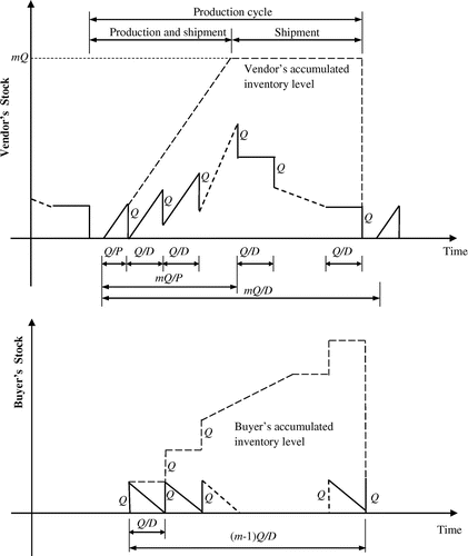
(2)	The buyer orders a lot of size Q and the vendor produces mQ units with a finite production rate P (P > D) in one production set-up but ships in quantity Q to the buyer over m times as shown in Figure 1.
(3)	Demand is deterministic.
(4)	Carbon emission is considered from production, inventory holding and transportation.

3.2. Development of mathematical models and solution techniques

Three mathematical models, namely carbon tax model, strict cap model and cap-and-trade model have been developed in a two-echelon SC. The basic objective of these models are finding the optimal order quantity and number of shipments between the vendor and buyer in each production cycle by minimizing the total SC cost while satisfying the basic bindings of the respective policies.

When the buyer orders a lot of size Q, the vendor begins production with a constant production rate P. The vendor produces the item in a lot of size mQ in each production cycle of length mQ/D. Initially, both production and shipments take place simultaneously for the first mQ/P units of time, after that the vendor stops the production and only continues shipments until the vendor’s inventory falls to zero. The buyer receives the supply in m lots each of size Q. The first lot of size Q is ready for shipment after Q/P units of time from the starting of the production, and then the vendor continues the delivery after every Q/D units of time. The inventory level at the buyer declines with a constant rate D. Accordingly, Figure 1 depicts the production, and inventory variation patterns at the vendor and the buyer, respectively.

The vendor’s average inventory is evaluated from Figure 1 as the difference of the vendor’s accumulated inventory and the buyer’s accumulated inventory, which is developed based on the model proposed by Joglekar (1988).

Vendor’s average inventory = 

3.3. Model I: carbon tax model

A carbon tax model can be of different forms. In its simplest form, the tax is a linear financial penalty, chargeable on every unit of carbon emission (Benjaafar, Li, and Daskin 2013). So, a pre-defined monetary unit is multiplied with every unit of carbon emission and added with other cost components for establishing the total supply chain cost.

We consider production, inventory and transportation as the major sources of carbon emissions. The expression for finding the emissions per unit time from all these sources is found as follows:

Carbon emission due to production per unit time = πD:

Adding all the emission components, the total emission per unit time is given by(1)

In the SC under consideration, the total cost function comprises the buyer’s ordering cost, vendor’s set-up and production costs, inventory holding costs at the vendor and buyer, transportation cost between the vendor and buyer and the total emission cost.

The vendor’s production setup and production costs per unit time = 

The vendor’s inventory holding cost per unit time = 

The buyer’s ordering and inventory holding costs per unit time = 

The transportation cost per unit time is calculated based on the number of trips made per unit time by the loaded and empty vehicle between the vendor and buyer, which is given by,

The total emission cost per unit can be determined by multiplying Equation (1(1) ) with tax T to be paid on each unit of carbon emission and is obtained as follows:

Thus, the total cost of the SC is obtained by adding all the above cost components, which is given by,(2)

3.3.1. Computation of the optimal order quantity

We have shown that TC (Q,m) is a convex function with respect to Q for fixed m in Appendix A. Therefore, the optimal value of Q for fixed m can be obtained by setting Equation (A.1(A.1) ) to zero, and we get(3)

Now, we have also shown that function TC(Q,m) is convex with respect to m for fixed Q in Appendix A. But, the way we have found the optimal Q cannot be implemented to determine the optimal value m due to integer restriction on m. Therefore, the procedure to determine the optimal value of m is presented below.

3.3.2. Determination of optimal number of shipments

Ignoring the terms, which are independent of Q and m in Equation (2(2) ), we can write:(4)

Putting the expression for Q from Equation (3(3) ) in the above equation, we get(5)

As minimizing is equivalent to minimization of the square of it, and so taking the square of Equation (5(5) ), we have,(6)

Simplifying further, we get(7)

Now, ignoring the terms that are independent of m, the minimization of

is equivalent to minimization of,(8)

Now, the optimal value of m will satisfy the following condition(9)

From Equation (9(9) ) we can derive the following condition(10)

Thus, the optimal value of m can be found using the condition given by (10), and then the optimal Q from Equation (3(3) ). Subsequently, the value of TE and TC can be determined from Equations (1(1) ) and (2(2) ), respectively.

3.4. Model II: strict carbon cap model

In case of strict carbon cap model, the penalty for exceeding the cap is infinitely large (Chen, Benjaafar, and Elomri 2013). So, companies are forced to manage their emission within the given limit. In this model, the objective is to minimize the sum of all the cost components, determined earlier, except the cost related to carbon emissions. Here, Ĉ is the total permissible carbon emission limit per unit time. Therefore, the total emission per unit time from the SC should be less than or equal to Ĉ. Now, the mathematical formulation of the strict carbon is given by(11) (12)

3.4.1. Computation of the optimal order quantity

If we temporarily ignore the emission constraint given by (12), we can determine the optimal value of Q that minimizes the total cost by proving TC(Q,m)as a convex function with respect to Q for fixed m (shown in Appendix B).Then, the optimal value of Q = Q₀ for fixed m is determined by setting the first derivative from Equation (B.1(B.1) ) to zero, and we have(13)

The above optimal order quantity for fixed m is derived ignoring the carbon emission constraint, and so Q₀ may not be a feasible order quantity. This Q₀ will be optimal for fixed m if the carbon emission constraint given by (12) is satisfied. Now, if the constraint is violated, then the constraint becomes active and we adopt the technique proposed by Chen, Benjaafar and Elomri (2013). For the purpose, we consider inequality (12) as an equation(14)

Now, Equation (14(14) ) can be expressed as a quadratic equation, and we can obtain two roots as follows:(15)

and(16)

where Q₁ and Q₂ are the lower and upper bounds, respectively, for feasible range of Q. Therefore, the optimal Q will be obtained using the following condition for fixed m.(17)

Equation (17(17) ) describes three possible cases: (i) when Q₀ falls in the feasible region, then optimal order quantity will take value as Q₀, which is the optimal value obtained from the total cost function; (ii) when Q₀ is smaller thanQ₁,the optimal order quantity becomesQ₁, as Q₁is the feasible point nearest to the optimal value obtained from the total cost function; similarly,(iii) when Q₀is larger thanQ₂, the optimal order quantity is given byQ₂. In the first case, the carbon constraint is inactive and the total emission is smaller than the carbon cap. In other two cases, the corresponding total cost will be larger than that of the first case.

3.4.2. Determination of initial value of number of shipments

In Appendix B we have also shown that TC(Q,m) is convex with respect to m for fixed Q. The optimal value of m should be derived considering each of the three possible values of Q as Q₀, Q₁ and Q₂ from condition (17(17) ) in the total cost expression similar to Model I. But, taking Q as Q₁ from Equation (15(15) ) or Q₂ from Equation (16(16) ) to express the total cost as a function of m will make the expression complicated. So, we have started with the similar approach adopted in model I to find an initial value of m that can be used to quickly search its optimal value. As TC(Q,m) is convex in m and takes integer value, therefore, the following condition must hold.(18)

From equation (18(18) ), we can derive the following condition(19)

On solving Equation (19(19) ), we can get an initial value of m.

Now, starting with the initial value of m, the following algorithm is developed to find the optimal value of Q and m.

3.5. Algorithm

Step 1: Find the integer value of m satisfying inequality (19).

Step 2: Find the value ofusing Equations (13(13) ), (15(15) ) and (16(16) ), respectively.

Step 3: Select the appropriate value of Q^m satisfying the condition in (17), and then find the corresponding.

Step 4: Repeat Steps (2) and (3) for to find TC (Q^m-1, m − 1), and TC (Q^m+1, m + 1), respectively.

Step 5: If m > 1 and , go to Step 6.

Else if , go to Step 7.

Else, set as the optimal solution and go to Step 8.

Step 6: Perform [6.1] to [6.3]

[6.1] Set m = m − 1

[6.2] Repeat Steps 2 and 3 to get

[6.3] Ifand m > 1go to [6.1]. Otherwise, set as the optimal solution and go to Step 8.

Step 7: Perform [7.1] to [7.3]

[7.1] Set m = m + 1

[7.2] Repeat Steps 2 and 3 to get

[7.3] If go to [7.1].Otherwise, set as the optimal solution and go to Step 8.

Step 8: Calculate and using Equations (20(20) ) and (1(1) ), respectively.

3.6. Model III: carbon cap-and-trade model

Under cap-and-trade policy firms are allowed to emit carbon within a specified level, which is called cap. If the firm crosses the cap during its operations, then the firm has to buy carbon credits from other firms. If the firm emits lower than the specified level, it earns carbon credit that can be sold to other firms.

We assume that the permissible limit of carbon emission is Ĉ per unit time. If the supply chain emits less than this limit, the excess amount is sold in the market. Also, if the actual emission is more than the permissible level then the additional amount of carbon needs to be bought from the market. We assume that the selling price and buying cost per unit of carbon is same, which is denoted as r (in monetary unit). The objective function to minimize the total cost of the supply chain can be formulated as follows:(20)

3.6.1. Computation of optimal order quantity

In Appendix C, we have shown that TC(Q,m) is a convex function with respect to Q for fixed m. Therefore, the optimal value of Q for fixed m can be obtained by setting Equation (C.1(C.1) ) to zero, and we have(21)

Now, we have also shown that function TC(Q,m) is convex with respect to m for fixed Q in Appendix C. But the way we have found the optimal Q cannot be implemented to determine the optimal value m due to integer restriction on m. Therefore, the procedure similar to model I for finding the optimal value of m is presented below.

3.6.2. Determination of optimal number of shipments

Ignoring the terms which are independent of Q and m, Equation (20(20) ) can be written as follows:(22)

Putting the value of Q from equation (21(21) ) in the above equation, we get(23)

As minimizing is equivalent to minimization of the square of it, and so taking the square of Equation (23(23) ), we have(24)

Simplifying further, we get(25)

Now, ignoring the terms that are independent of m, the minimization of is equivalent to minimization of(26)

Now, the optimal value of m will satisfy the following condition(27)

From Equation (27(27) ), the following condition can be derived(28)

Thus, the optimal value of m can be found using the condition given by (28), and then the optimal Q from Equation (21(21) ). Subsequently, the value of TE and TC can be determined from Equations (1(1) ) and (20(20) ), respectively.

4. Numerical examples and sensitivity analyses

To illustrate the proposed models and solution procedures, a two-stage SC is considered with the following data: D = 600 units/year, p = 2000 units/year, A = $200/order, S = $1500/setup, d = 100 km, v = 50 km/h, p = $200/unit, π = 3 ton/unit, h_b = $5/unit/year, h_v = $2/unit/year, t₀ = $10/h, t_Q = $5/unit/h, α_b = 0.80 ton/unit/year, α_v = 0.80 ton/unit/year, τ₀ = 0.03 ton/h, τ_Q = 0.004 ton/unit/h, T = $37/ton, r = $37/ton.

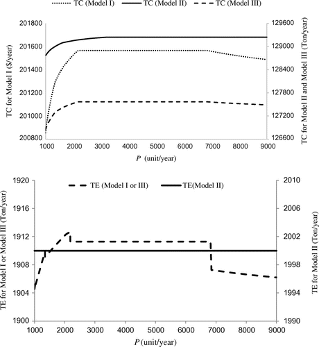
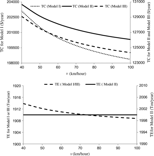
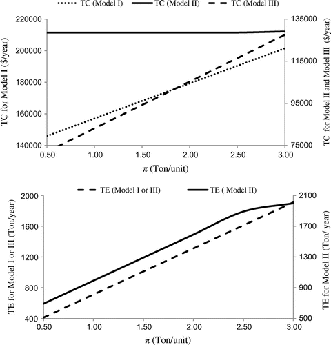
Now using the procedures discussed earlier, we can determine the optimal values of Q and m, and the corresponding TC and TE for three different models, respectively. The base case values of Q, m, TC and TE for all the models are given in Table 1. Next, we have conducted sensitivity analysis to examine how TCs and TEs of the models are changed with different values of the parameters. We have kept carbon tax rate (T) and carbon cost (r) same to facilitate the comparison between Model I and Model II and found that when T and r are same, TE for both the cases will be same but TC will be different, because in Model I, organizations will pay for every unit of emission whereas in case of Model III, organizations will start paying only after crossing a threshold level (Ĉ) and if the organizations emit within the given limit, they can also sell it. So, TEs for both Model I and Model III have been represented by a common line for sensitivity analyses. As far as TCs are considered, we have found a considerable difference between TC of Model I and TCs of Model II and Model III. Therefore, TC for Model I and TCs for Model II and Model III are plotted in different vertical axes. For the sensitivity analyses, we have considered only the important parameters which may provide some good insights.

Table 1. Base case solutions for the three different models.

Model	Q	m	TC	TE
I	99.06	3	201526.53	1912.15
II	180.56	3	129150.94	2000.00
III	99.06	3	127526.53	1912.15

Figure 2 shows the relationship of TCs and TEs with P. With the increasing value of P, Q keeps on changing and m goes up gradually. Initially the changing rate of m is much faster and subsequently m remains unchanged for a long interval that results initial surge in TC and after that TC remains almost unchanged. As far as the values of TEs are concerned, one can see that within the given range of P, the carbon constraint remains active throughout for the Model II. So, it is quite obvious that organization will utilize its given quota of carbon to attain minimum cost. So, TE will remain unchanged and always will be equal to the given carbon limit for Model II, but for Model I and Model III, it will increase with the increasing value of P, then remain unchanged but will come down sharply after a threshold level. But, we can conclude that TCs and TEs will be minimum at the lowest possible value of P.

Figure 2. Effects of P on TC and TE.

Figure 3 describes the changes of TCs and TEs with v. As v is inversely related to TC for all the three models, with increasing v, TCs will come down and TEs for Model I and Model III also show the same pattern (as v is also inversely related with TE). But, due to binding constraint, TE for Model II will remain unchanged as within our given range of v carbon constraint remains active.

Figure 3. Effects of v on TC and TE.

Figure 4 depicts the sensitivity of TCs and TEs with respect to π. With increasing value of π, TCs for all the three models will go up (though in case of Model II, it is very small) as π is directly proportional with TCs and it also holds true for TEs. Here, initially with lower π, the emission will be so less that for Model II carbon constraint will remain inactive. Therefore, initially for all the three cases, TEs will increase linearly, but in case of Model II, once carbon constraint becomes active, there will be no further change in TE.

Figure 4. Effects of π on TC and TE.

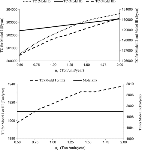
Figure 5 shows the change of TCs and TEs with α_v. As this parameter is also directly proportional to TCs and TEs, except for Model II for TE, all the other TCs and TEs will increase with increasing value of α_v. Due to strict binding on carbon, TE for Model II will remain unchanged. Similar variation in pattern of TC and TE can be observed by varying the value of α_b.

Figure 5. Effects of α_v on TC and TE.

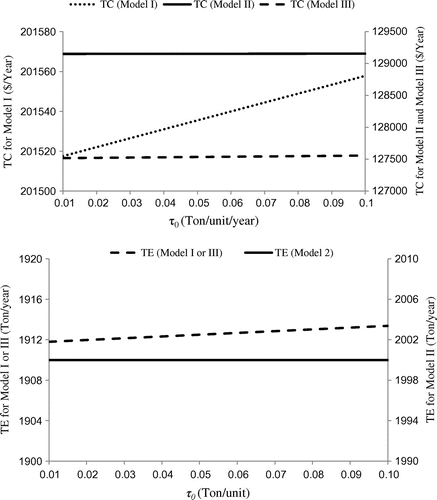
Figure 6 shows the change of TCs and TEs with τ₀. While considering the changing pattern of TCs, we observe very negligible increase in TCs with the increasing of τ₀, as because within the given range of τ₀, no change in value of m is taking place and the variation of Q is very low. The change of TEs in case of Model I and Model III is nominal and again one can observe that there is no change in TE for Model II. Similar variation in pattern of TC and TE can be observed by varying the value of τ_Q.

Figure 6. Effects of τ₀ on TC and TE.

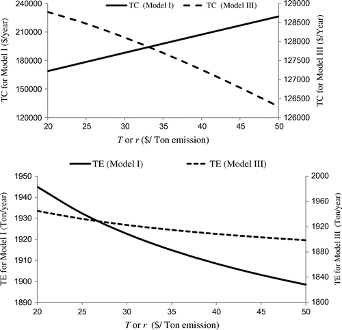
Figure 7 describes the effect of T for Model I and r for Model III on TC and TE. This figure provides some interesting managerial insights. When T or r increase, quite obviously firms will try to reduce their emission and as we discussed earlier, the total emission (TE) in Model I and Model III will be same (though here we have shown in two different vertical axes to avoid coinciding). But, for the set of values we have chosen, even when the emission will come down, the organization will incur more cost with T as it is totally linearly proportional with TC and also the changing rate of TC is quite high. But in case of Model III when the emission comes down, the organization also gets chance to sell of its unutilized carbon quota outside. Therefore, organization operating under carbon cap-and-trade will also be financially beneficial.

Figure 7. Effects T or r on TC and TE.

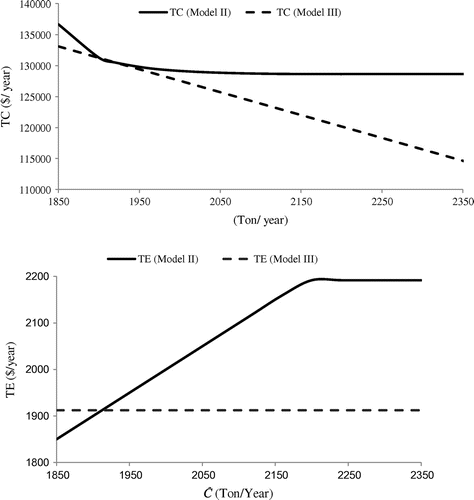
Figure 8 depicts the effect of Ĉ on TC and TE in Model II and Model III. With increasing Ĉ, constraint for Model II will be relaxed and organizations will keep on emitting. In strict carbon cap policy (Model II) organizations cannot emit carbon beyond the given level, but if the constraint is relaxed, it helps organization to minimize their cost as they can optimize their operations with relaxed constraint. So, with increasing Ĉ (relaxing of constraint) initially, TC will come down and organization will start emitting more carbon and TE will go up. But, beyond a certain range, organizations don’t need to emit more to reduce cost and if allotted Ĉ is more than or equal to the range, it will have no impact on TC and TE. For Model III, there will be no impact of Ĉ on TE, as with increasing Ĉ, the carbon constraint will be more relaxed and organizations will optimize their operations without bothering about carbon constraint. But their cost will come down as they will be able to sell unutilized quota of carbon in the market.

Figure 8. Effects Ĉ on TC and TE.

5. Conclusion, limitations and future scope

In this paper, we consider a two-echelon SC consisting of a single vendor and a single buyer. In practice this model is useful for a firm having two separate divisions, where the firm as a single owner of both the divisions tries to reduce total cost and total emission for the entire operations. We have considered here infinite time period, and explicitly considered emissions from all the major sources in SC, namely – production, inventory handling and transportation. We develop models to minimize the total cost of the vendor–buyer integrated system by simultaneously optimizing the ordering quantity and the number of shipments from the vendor to the buyer in a production cycle. We also present numerical examples and sensitivity analyses. Our models are useful to compare different carbon policies for vendor–buyer integrated supply chain.

This paper has shown that it is quite easy for organizations to operate under carbon tax and carbon cap-and-trade policies. Companies face most difficulties under strict carbon cap policy and many times organizations cannot attain optimal cost due to carbon constraint. If any organization fails to restrict their emission within the specified carbon emission limit, they will be ended up with closing down their business. Carbon cap-and-trade gives the flexibility to trade carbon in the market and also encourage organization to emit less. In reality, carbon policies based on carbon tax or cap-and-trade are practiced mainly as they are more flexible. But, the strict carbon cap policy always restricts emission within a desired level proposed by the regulatory bodies. Emissions under carbon tax and carbon cap-and-trade policies can vary depending corresponding carbon tax (T) or buying/selling price of carbon (r). Depending on the allotted carbon level the emission under strict carbon cap policy can be less or more comparing to the emissions take place under carbon cap policy or carbon cap-and-trade policy.

This paper considers a simple two stage supply chain. A more complex and realistic supply chain could be considered in future study. Here, we have assumed that the product, taken into consideration is general normal goods. But, as emissions from different sources are product dependent, a significant change can be witnessed in sensitivity analysis if we consider specific product. We have assumed a simple tax pattern for first model. In reality the tax structure could be more complex.

Scope for future research is numerous. In future one can consider finite planning period. Our model is based on economic production quantity model; one can extend it for other inventory models. A reverse supply chain with defective and waste item also could be considered. Hybridizing different models could be another interesting area to explore.

Disclosure statement

No potential conflict of interest was reported by the authors.

Appendix A

From Equation (2(2) ), we have

Finding the first and second partial derivatives of TC(Q, m) with respect to Q for fixed m, we get(A.1)

and(A.2)

Hence, TC(Q, m) is convex with respect to Q for fixed m.

Now, temporarily relaxing the integer requirement on m, we find the first and second partial derivatives of TC(Q, m) with respect to m for fixed Q and get(A.3)

and(A.4)

So, TC(Q, m) is convex with respect to m for fixed Q.

Appendix B

From Equation (11(10) ),

Finding the first derivative of TC(Q,m) with respect to Q for fixed m, we have(B.1)

Since, TC (Q, m) is convex in Q for fixed m, because(B.2)

Now, temporarily relaxing the integer requirement on m, TC(Q, m) is convex in m for fixed Q, because(B.3)

Appendix C

From Equation (20(20) ), we have

Finding the first and second partial derivatives of TC(Q, m) with respect to Q for fixed m, we get(C.1)

and(C.2)

Hence, TC(Q, m) is convex with respect to Q for fixed m.

Now, temporarily relaxing the integer requirement on m, we find the first and second partial derivatives of TC(Q, m) with respect to m for fixed Q and get(C.3)

and(C.4)

So, TC(Q, m) is convex with respect to m for fixed Q.

References

- Abdallah, T., A. Diabat, and D. Simchi-Levi. 2010. “A Carbon Sensitive Supply Chain Network Problem with Green Procurement.” Proceedings of the 40th International Conference on Computers and Industrial Engineering (CIE), Awaji, Japan, July 25–28, 2010. 10.1109/ICCIE.2010.5668278.
- Abhishek, N., M. B. Nidhi, and V. M. Pillai. 2012. “Carbon Assessment Model for Supply Chain Network.” Proceeding of the International Conference on Green Technologies (ICGT), Trivandrum, India, December 18–20, 2010. 10.1109/ICGT.2012.6477995.
- Absi, N., S. Dauzère-Pérès, S. Kedad-Sidhoum, B. Penz, and C. Rapine. 2012. “Lot Sizing with Carbon Emission Constraints.” European Journal of Operational Research 227 (1): 55–61. 10.1016/j.ejor.2012.11.044.
- Benjaafar, S., Y. Li, and M. Daskin. 2013. “Carbon Footprint and the Management of Supply Chains: Insights from Simple Models.” IEEE Transactions on Automation Science and Engineering 10 (1): 99–116. 10.1109/TASE.2012.2203304.
- Bouchery, Y., A. Ghaffari, Z. Jemai, and Y. Dallery. 2012. “Including Sustainability Criteria into Inventory Models.” European Journal of Operational Research 222 (2): 229–240. 10.1016/j.ejor.2012.05.004.
- Carbon Trust. 2006. “Carbon Footprint in the Supply Chain: The Next Step for Business.” Carbon Trust, Accessed September 30, 2013. https://www.carbontrust.com/media/84932/ctc616-carbon-footprints-in-the-supply-chain.pdf.
- Carter, C. R., and D. S. Rogers. 2008. “A Framework of Sustainable Supply Chain Management: Moving toward New Theory.” International Journal of Physical Distribution & Logistics Management 38 (5): 360–387. 10.1108/09600030810882816.
- Carter, C. R., and P. L. Easton. 2011. “Sustainable Supply Chain Management: Evolution and Future Directions.” International Journal of Physical Distribution & Logistics Management 41 (1): 46–62. doi:10.1108/09600031111101420.
- Chen, W. T., Y. P. Li, G. H. Huang, X. Chen, and Y. F. Li. 2010. “A Two-stage Inexact-stochastic Programming Model for Planning Carbon Dioxide Emission Trading under Uncertainty.” Applied Energy 87 (3): 1033–1047. 10.1016/j.apenergy.2009.09.016.
- Chen, X., S. Benjaafar, and A. Elomri. 2013. “The Carbon-Constrained EOQ.” Operations Research Letters 41 (2): 172–179. 10.1016/j.orl.2012.12.003.
- Ciliberti, F., P. Pontrandolfo, and B. Scozzi. 2008. “Logistics Social Responsibility: Standard Adoption and Practices in Italian Companies.” International Journal of Production Economics 113 (1): 88–106. 10.1016/j.ijpe.2007.02.049.
- Darnall, N., G. J. Jolley, and R. Handfield. 2008. “Green Supply Chain Management: Complements for Sustainability?” Business Strategy and the Environment 45 (18): 30–45. 10.1002/bse.557.
- Dekker, R., J. Bloemhof, and I. Mallidis. 2012. “Operations Research for Green Logistics – An Overview of Aspects, Issues, Contributions and Challenges.” European Journal of Operational Research 219 (3): 671–679. 10.1016/j.ejor.2011.11.010.
- Dheeraj, N., and N. Vishal. 2012. “An Overview of Green Supply Chain Management in India.” Research Journal of Recent Sciences 1 (6): 77–82.
- Diabat, A., and D. Simchi-Levi. 2009. “A Carbon-capped Supply Chain Network Problem.” Proceedings of the IEEE International Conference of on Industrial Engineering and Engineering Management, Hong Kong, December 8–11. 10.1109/IEEM.2009.5373289.
- Dobos, I. 2005. “The Effects of Emission Trading on Production and Inventories in the Arrow-Karlin Model.” International Journal of Production Economics 93–94: 301–308. 10.1016/j.ijpe.2004.06.028.
- Dobos, I. 2007. “Tradable Permits and Production-Inventory Strategies of the Firm.” International Journal of Production Economics 108 (1–2): 329–333. 10.1016/j.ijpe.2006.12.039.
- Dong, C., B. Shen, P. S. Chow, L. Yang, and C. T. Ng. 2016. “Sustainability Investment under Cap-and-Trade Regulation.” Annals of Operations Research 240 (2): 509–531. doi:10.1007/s10479-013-1514-1.
- ET Bureau. Market-friendly Pollution Control System Launched. 2011. The Economics Times, March 26. http://articles.economictimes.indiatimes.com/2011-03-26/news/29192418_1_emission-trading-emission-levels-pollution-control.
- Fahimnia, B., J. Sarkis, F. Dehghanian, N. Banihashemi, and S. Rahman. 2013. “The Impact of Carbon Pricing on a Closed-loop Supply Chain: An Australian Case Study.” Journal of Cleaner Production 59: 210–225. 10.1016/j.jclepro.2013.06.056.
- Giunipero, L. C., R. E. Hooker, and D. Denslow. 2012. “Purchasing and Supply Management Sustainability: Drivers and Barriers.” Journal of Purchasing & Supply Management 18 (4): 258–269. 10.1016/j.pursup.2012.06.003.
- Gold, S., S. Seuring, and P. Beske. 2010. “Sustainable Supply Chain Management and Inter-Organizational Resources: A Literature Review.” Corporate Social Responsibility and Environmental Management 17 (4): 230–245. 10.1002/csr.207.
- Hammami, R., I. Nouira, and Y. Frein. 2015. “Carbon Emissions in a Multi-Echelon Production-Inventory Model with Lead Time Constraints.” International Journal of Production Economics 164: 292–307. 10.1016/j.ijpe.2014.12.017.
- Hoen, K. M. R., T. Tan, J. C. Fransoo, and G. J. van Houtum. 2014. “Effect of Carbon Emission Regulations on Transport Mode Selection under Stochastic Demand.” Flexible Services and Manufacturing Journal 26 (1): 170–195. 10.1007/s10696-012-9151-6.
- Hua, G., T. C. E. Cheng, and S. Wang. 2011. “Managing Carbon Footprints in Inventory Management.” International Journal of Production Economics 132 (2): 178–185. 10.1016/j.ijpe.2011.03.024.
- Jaber, M. Y., C. H. Glock, M. A. Ahmed, and E. I. Saadany. 2013. “Supply Chain Coordination with Emissions Reduction Incentives.” International Journal of Production Research 51 (1): 69–82. 10.1080/00207543.2011.651656.
- Joglekar, P. N. 1988. “Comments on ‘a Quantity Discount Pricing Model to Increase Vendor Profits’.” Management Science 34 (11): 1391–1398. 10.1287/mnsc.34.11.1391.
- Kelle, P., and E. Silver. 1989. “Forecasting the Returns of Reusable Containers.” Journal of Operations Management 8 (1): 17–35. 10.1016/S0272-6963(89)80003-8.
- Kinaxis. 2009. “Providing Carbon Footprint Visibility and Planning Capabilities across the Supply Chain: Why You Need to Do It and What You Need to Do It” White Paper. Kinaxis, Canada. Accessed December 28, 2012. http://www.kinaxis.com/downloads/register/WP-Carbon_Footprint_Planning_Capabilities.pdf.
- Labatt, S., and R. White. 2007. Carbon Finance: The Financial Implications of Climate Change. Hoboken: John Wiley & Sons.
- Li, S. 2013. “Optimal Control of the Production–Inventory System with Deteriorating Items and Tradable Emission Permits.” International Journal of Systems Science 45 (11): 2390–2401. 10.1080/00207721.2013.770103.
- Metcalf, G. E. 2009. “Market-Based Policy Options to Control U.S. Greenhouse Gas Emissions.” Journal of Economic Perspectives 23 (2): 5–27. 10.1257/jep.23.2.5.
- Mitra, S., and P. P. Datta. 2013. “Adoption of Green Supply Chain Management Practices and Their Impact on Performance: An Exploratory Study of Indian Manufacturing Firms.” International Journal of Production Research 52 (7): 1–23. 10.1080/00207543.2013.849014.
- Morgenstern, R. D. 2002. Reducing Carbon Emissions and Limiting Costs. Washington, DC: Resources for the Future. http://www.aspeninstitute.org/sites/default/files/content/docs/ee/MorgensternEEEClimate.pdf.
- Pagell, M., and Z. Wu. 2009. “‘Building a More Complete Theory of Sustainable Supply Chain Management Using Case Studies of 10 Exemplars’.” Journal of Supply Chain Management 45 (2): 37–56. 10.1111/j.1745-493X.2009.03162.x.
- Ramudhin, A., A. Chaabane, M. Kharoune, and M. Paquet. 2008. “Carbon Market Sensitive Green Supply Chain Network Design.” IEEE International Conference on Industrial Engineering and Engineering Management 5 (1): 1093–1097. 10.1109/IEEM.2008.4738039.
- Rosič, H., and W. Jammernegg. 2013. “The Economic and Environmental Performance of Dual Sourcing: A Newsvendor Approach.” International Journal of Production Economics 143 (1): 109–119. 10.1016/j.ijpe.2012.12.007.
- Seuring, S., and M. Müller. 2008. “From a Literature Review to a Conceptual Framework for Sustainable Supply Chain Management.” Business Strategy and the Environment 17 (8): 455–466. 10.1016/j.jclepro.2008.04.020.
- Srivastava, S. K. 2007. “Green Supply-Chain Management: A State-of the Art Literature Review.” International Journal of Management Reviews 9 (1): 53–80. 10.1111/j.1468-2370.2007.00202.x.
- Srivastava, S. K., and R. K. Srivastava. 2006. “Managing Product Returns for Reverse Logistics.” International Journal of Physical Distribution & Logistics Management 36 (7): 524–546. 10.1108/09600030610684962.
- Svensson, G. 2007. “Aspects of Sustainable Supply Chain Management (SSCM): Conceptual Framework and Empirical Example.” Supply Chain Management: An International Journal 12 (4): 262–266. 10.1108/13598540710759781.
- Swami, S., and J. Shah. 2013. “Channel Coordination in Green Supply Chain Management.” Journal of the Operational Research Society 64 (3): 336–351. 10.2139/ssrn.2120414.
- WHO (World Health Organization). 2015. “Climate Change and Health.” Accessed February 5, 2016. www.who.int/mediacentre/factsheets/fs266/en/.
- Zhang, B., and L. Xu. 2013. “Multi-item Production Planning with Carbon Cap and Trade Mechanism.” International Journal of Production Economics 144 (1): 118–127. 10.1016/j.ijpe.2013.01.024.
Appendix A
From Equation (Equation2(2) ), we have