Time and cost characterisation of emissions from non-road diesel equipment for infrastructure projects

Abstract

The construction process contributes to pollutant emissions, particularly through the operation of diesel- and gasoline-powered equipment. In the past decade, a series of investigations were undertaken to quantify these emissions for a variety of non-road construction equipment performing different activities and undergoing different duty cycles, and a model to estimate quantities of six types of pollutant was developed. This paper uses that model to estimate emissions for four street and utility construction projects which no one has done previously. We combined information from company records with standard construction industry manuals to estimate total emissions for the projects and to examine the pollution patterns and magnitudes. The street construction projects all had similar emission profiles with a large peak at the beginning and a steady output of emissions throughout the duration of the project. For example, in two of the projects studied, half of all CO₂ emissions were produced before the projects were 40% completed. Results showed that demolition and earthwork are the activities with the largest contribution. The equipment types with the largest contribution are backhoes, front-end loaders, bulldozers and trenchers. Trenchers, for example, produced 30% of all emissions on the projects on which they were used.

Keywords:

• Construction equipment
• air pollutants
• emissions
• transportation construction projects
• construction emissions
• emissions forecasting
• construction activities

Introduction

The construction industry is ranked third in greenhouse emissions compared to other industry sectors in the US (EPA 2008). Emissions from construction are equivalent to 6% of the greenhouse emissions from all industries in the US. Of the 131 million metric tons of CO₂ equivalent that construction produced in 2002, 100 million tons (or 76%) are due to fossil fuel combustion. Thus, reducing emissions from construction equipment is an important step toward cleaner air on a national level.

Tatari and Kucukvar (2012) studied the ecological impact of the construction industry. From the 13 sectors in which the construction industry was divided, highway construction was ranked fifth in total industry output in dollars. However, highway construction and highway maintenance had the highest CO₂ emissions per dollar of economic output.

Recent regulations by the US Environmental Protection Agency (EPA) for non-road vehicles and equipment have focused on the manufacturers of the engines used. However, the new regulations only apply to equipment that is manufactured after a specific regulation comes into effect. Each new set of emissions regulations is referred to as a tier and is used as a means to identify the engines with respect to their emissions level. For example, engines that comply with the first regulation in 1996 are known as Tier 1 engines. Engines manufactured before the regulations were in place are classified as Tier 0 engines. Tier 4 regulation will be fully implemented in 2015 (EPA 2010b).

EPA developed the NONROAD model which provides emission factors for non-road equipment according to engine size, engine tiers and equipment type. The pollutants that were used for this study are those classified as exhaust pollutants by the NONROAD model and include hydrocarbons (HC), nitrogen oxides (NO_x), carbon monoxide (CO), particulate matter (PM), sulphur dioxide (SO₂) and carbon dioxide (CO₂).

The Clean Air Act requires EPA to develop National Ambient Air Quality Standards for criteria pollutants; those pollutants that negatively affect human health and the environment (EPA 2013). Four of the pollutants (noted above) that we investigate herein (CO, NO_x, PM and SO2) are criteria pollutants. HC emissions are important because they participate in the atmospheric process that produces ozone, another of the criteria pollutants. CO₂ is studied regularly because it is a greenhouse gas and likely contributes to climate change.

Problem statement

Highway construction, rehabilitation and resurfacing have a significant environmental impact due to emissions primarily from the use of diesel-powered equipment. However, there has not been an established methodology for estimating construction activity emissions at the project or activity levels for street and utility construction projects.

This paper contributes one such methodology – a direct link between street construction activities and emissions. Such a methodology can enable contractors and fleet managers to estimate the emissions from their equipment without the need to field measure emissions from every item of equipment used and then knowing the environmental impact only after the fact. Instead, the key goal is to have a methodology to estimate project emissions during planning and preliminary engineering project stages.

The main objective of this paper is to present a methodology for engineers and contractors to estimate the total emissions from a specific type of very common transportation construction project – street and utility projects. The use of this methodology is illustrated by its application to four projects, thereby providing quantified emissions predictions for various levels of detail that can be assessed and used for further study. Two of the projects include pavement rehabilitation and utility work on an existing street. The other two projects (two separate phases) include street construction and utility work for a new residential subdivision. Their objectives were to evaluate the adequacy of emissions data sources and to assess patterns of emissions during typical transportation construction projects. Furthermore, we also sought a way to obtain accurate estimates that could be used as inputs to the various life cycle models that are prevalent.

The projects studied herein are representative of the type of construction that is regularly completed by local governments and developers; thus, the results of the paper have broad practical applications. It is important to realise that all levels of government and private developers commonly perform this work. The literature search revealed that street and utility projects have not previously been studied. Contractors and local agencies can use this work to estimate emissions from these types of projects.

Literature review

Various studies have been performed to determine the effect of construction activities on the environment. The construction industry includes numerous project types that range from residential to industrial buildings and from large industrial projects to mega infrastructure projects. Those projects may range from small-scale endeavours that cost only a few thousand dollars to large-scale ‘megaproject’ that exceeds one billion dollars in cost.

One of the ways to study the pollutants emissions of various construction projects is by analysing the life cycle of the projects. There is a rich literature on life cycle analysis for infrastructure projects (Bilec et al. 2010; Guggemos and Horvath 2006; Junnila et al. 2006). However, none of that literature addresses the problem presented in this paper. The emissions are often calculated for all the phases of the life cycle of a project, including material manufacturing and transportation, construction, operation, maintenance and demolition and disposal. One such study showed that the construction phase accounts for 6% of the total energy consumption and 9% of the total equivalent CO₂ emissions for residential projects in Canada. The operation phase accounted for the remaining 94% of the energy consumption and 91% of the equivalent CO₂ emissions (Baouendi, Zmeureanu, and Bradley 2005). Another study showed that asphalt and bridge repair projects produced 3.5 times more NO_x than did building projects (Sharrard, Matthews, and Ries 2008). A study by Lee et al. (2011) concluded that projects that use recycled materials improved sustainability and reduced greenhouse gas emissions.

Kim et al. (2012) developed a methodology to estimate CO₂ emissions from road construction activities. The methodology had three basic steps: estimate working hours of the equipment, calculate fuel use for those hours and calculate greenhouse gas quantities based on equipment fuel consumption. The activities were divided into earthwork, pavement, utility and miscellaneous. It was determined that earthwork activities used more fuel than any of the other activities. For the majority of the cases dump trucks emitted the greatest quantity of pollutants.

Some studies directly measured emissions from equipment while working on site. The study by Lewis, Frey and Rasdorf (2009) presented an emissions inventory using actual emissions measurements from equipment fleets. This paper focused on emissions inventories for equipment but not project activities. The equipment was tested using both petroleum diesel and a biodiesel blend (B20). The results showed that emissions were lower for equipment using biodiesel as fuel. The inventory also showed that emissions were lower for higher tier equipment. As a result of this study, the NCDOT converted its entire fleet to biodiesel fuel.

The emissions inventory resulting from the Lewis study was used to develop a set of practices that the construction industry can use to reduce emissions (Lewis et al. 2009). The recommended practices included the improvement of maintenance procedures, the use of alternative fuels and the development of emissions inventories based on accurate emissions estimates. Other opportunities to reduce emissions were also presented by EPA (2009). The actions by the contractors with the most influence in reducing greenhouse gases emissions were determined to be fuel selection, equipment maintenance, equipment idling, equipment selection, electricity used and materials recycling.

Lewis et al. (2012) also studied the effect of productivity and idling time on total emissions. The authors concluded that emissions were considerably lower during idle time. However, idling has a negative effect on productivity and results in an overall increase in emissions for a particular activity or project.

A methodology was presented by Marshall et al. (2012) to estimate emissions from building construction projects and was used to estimate emissions from a small commercial project. The authors calculated the emissions for each individual construction activity using project data (and a project schedule provided by the contractor) that were combined with crew, productivity and cost data from Means (2013). Results from this study showed that concrete work was responsible for 45% of the total CO emissions, that the most emissions were generated early in the construction process, and that those emissions were primarily due to earthwork and site preparation activities (thus verifying the findings of Kim et al. 2012).

Previous work had shown that emissions from road construction projects are significant. These emissions can be changed by taking equipment and fuel characteristics into consideration. It was also shown that equipment use (particularly idle time) has an impact on total emissions from infrastructure projects. What was missing in the previous literature was a methodology that contractors and local governments could use to estimate these emissions. It was our intention in this study to provide this methodology and we do so herein. This paper introduces emissions estimates and metrics for street and utility infrastructure projects. Furthermore, the data used herein are available for further study by other researchers for future project type comparisons.

Methodology

A methodology was previously developed and tested on a commercial building project (Marshall et al. 2012). The methodology was initially designed to be easily implemented by construction professionals. In this paper, the authors sought herein to apply, refine and assess the methodology in a transportation construction setting. Highway and building projects likely differ in emissions patterns because highway projects involve earthwork throughout the duration of the project and because highway projects involve paving, for example. Both earthwork and paving are heavy emissions producers. Plans, specifications, equipment fleet composition, fuel use and other data were obtained for the four transportation street construction projects described above.

Data sources

The project data presented here were developed using both the EPA’s NONROAD Model and RS Means estimating data. The contractor that worked on the four projects described and analysed herein provided basic project characteristics, schedule, cost and equipment used for each activity as well as basic equipment characteristics. Additional data were collected from the equipment manufacturer’s manuals. An abundance of actual field data was available and was made use of. This section explains how these data sources were obtained for this project. For a further discussion of additional data sources see Marshall et al. (2012).

EPA has developed a widely used NONROAD model to estimate emissions from all types of non-road equipment (EPA 2005). The model allows the user to select the different types of engines and different localities for their use. It supports equipment use classifications including agriculture, marine, construction and others. The EPA NONROAD Model provides emission factors for equipment based on differing equipment characteristics.

Pollutant emission factors in the NONROAD model are dependent on equipment type, engine tier and type of fuel. The pollutant emission factors are provided in grams of pollutant per horsepower hour. In addition to the factors themselves, we used further adjustments for each item of equipment that took into consideration the deterioration of the engine and the engine load. The adjustments were completed following the methodology provided by EPA (2010a).

RS Means provides estimates of crew, cost and productivity data for typical construction activities (Means 2013). These data items were used to estimate the project schedule, cost and equipment needs of each project activity using data usually available to contractors during the early phases of the project.

A key goal of this paper is to present the results using this published data in conjunction with field data to estimate emissions production on equipment and activity levels using the best information available. In doing so, the results and insights gained can be used to provide more precise data as input to life cycle models. Presently, life cycle models use estimates rather than detailed equipment emissions data.

Project descriptions

Street construction projects can primarily be divided by project type into new construction, rehabilitation and resurfacing. The four projects presented here focus on street and utility rehabilitation construction projects, including new pavement placement. These projects represent typical construction work regularly performed by construction companies for city streets and residential developments. This kind of construction is prevalent throughout the US, especially in rapidly growing areas.

Four projects were selected to represent small street projects. These types of projects usually include work to improve or relocate utilities and curbs. A construction firm that specialises in street construction provided the plans and specifications, the schedule and insight into the field construction methods used.

The projects consisted of two separate street rehabilitation projects and one other subdivision street construction project delivered in two phases (referred to herein as two separate projects). Table 1 shows basic characteristics of the four projects and Table 2 shows the construction activities associated with each project. The costs calculated for all the projects and activities were determined using Means (2013) cost data.

Table 1. Project characteristics.

Project	Acronym	Total cost	Year built	Construction duration (days)	Length (ft)	Width (ft)	Description
Little Street Roadway	LS	$179,000	2011	65	600	24	Street and utility improvement
W. Burkhead Street	WB	$103,860	2012	9	500	27	Street and utility improvement
Sutton Place Phase 1	SP1	$219,540	2009	49	930	20	New development
Sutton Place Phase 2	SP2	$622,660	2009	101	2813	27	New development

Table 2. Project construction activities.

Construction activities	Projects
	Little Street	West Burkhead	Sutton Place Phase 1	Sutton Place Phase 2
Mobilisation	X	X	X	X
Staking and layout	X	X	X	X
Clearing and grubbing			X	X
Demolition and removal of existing asphalt	X	X
Erosion control measures			X	X
Earthwork and grading			X	X
Demolition of sewer, storm, and water systems	X
Initial grading and excavation		X
Installation of new sanitary sewer system	X	X	X	X
Abandon existing sewer		X
Installation of water distribution system	X		X	X
Installation of storm sewer	X		X	X
Remove and replace curb on adjacent streets		X
Prepare subgrade	X	X	X	X
Paving	X	X	X	X
Final clean up, punch list and demobilisation	X	X	X	X

Calculation steps

The general methodology consists of performing a quantity take-off, developing a cost estimate, assembling emission factors, developing and undertaking an activity level emissions analysis, and developing overall project level emissions estimates.

The first step was to benchmark the information supplied by the contractor. The project schedule is part of the contract documents and was determined to be reliable. The contractor identified the items of equipment used for the construction project. The hours of operation for the equipment were estimated using labour hours provided by the contractor for each construction activity. However, while labour hours provided an estimate of the amount of time the equipment was located at the job they did not necessarily provide a good estimate of the number of hours that the equipment was in use. In cases where contractor data were insufficient to determine the characteristics of the equipment used for each activity, RS Means data (2013) were used to supplement the contractor’s data.

The activities in the contractor’s schedule were matched with a corresponding activity or group of activities from RS Means. Some of the activities were directly equivalent to an activity in RS Means, others required a grouping of similar or multiple activities.

In addition to cost and productivity data, RS Means also identifies a specific crew composition for each activity including the labourers and equipment operators as well as the items of equipment required to perform the activity. For most of the equipment identified, RS Means also provided its engine size (in horsepower) and its capacity (e.g. cubic yards).

A final project schedule was developed using the most reliable information from all the sources. The activities and total duration were determined using information from the contractor. The list of equipment and total hours of use, as well as the total cost, were determined using RS Means. The activity duration was adjusted to fit the actual field schedule provided by the contractor. Doing so reflected the actual delays and other situations that the contractor encountered during the construction process.

Once a final schedule was determined, the emission factors for the items of equipment were obtained from the EPA NONROAD model. Table 3 shows the equipment that was determined using RS Means and used on all four projects. The table includes equipment type, horsepower, emission factors and the projects on which each item of equipment was used. The emission factors were adjusted assuming that all the equipment used was Tier 2. Tier 2 equipment was produced during the years 2003 to 2007 and it is reasonable to assume that the typical equipment used by small contractors was obtained before the economic downturn of 2008. EPA default values were used for the other information needed to adjust the emission factors for deterioration of the engine and variance on the actual use of the engine.

Table 3. Project pollutant emissions rates for Tier 2 equipment (EPA 2010a, 2010b).

Equipment type	HP	Emissions factors (g/hp-hr)						Projects
		HC	CO	NOx	PM	CO2	SO2	LS	WB	SP1	SP2
Asphalt paver	130	0.48	4.0	5.18	0.72	4670	0.82	X	X	X	X
Backhoe loader	48	1.70	11.55	7.26	0.41	5160	0.91	X	X	X	X
Brush chipper	110	0.65	2.83	6.62	0.57	4620	0.81	X
Concrete pump	400	0.49	3.56	6.59	0.62	4620	0.81	X	X
Curb paver	130	0.60	5.25	5.60	0.83	4660	0.82	X
Bulldozer	105	0.42	3.79	5.42	0.61	4670	0.82	X	X	X	X
Front end loader	80	1.70	11.55	7.26	0.41	5160	0.91	X	X	X	X
Grader	138	0.39	2.77	4.97	0.56	4670	0.82	X	X	X	X
Horizontal directional drill	100	0.49	3.55	6.58	0.61	5140	0.90	X
Hydraulic crane	130	0.42	1.63	6.21	0.36	4620	0.81	X
Hydraulic excavator	160	0.39	3.13	4.96	0.61	4670	0.82	X	X	X	X
Pneumatic roller	100	0.55	4.86	5.31	0.81	5190	0.91	X	X	X
Self-propelled crane	200	0.42	1.72	6.24	0.44	4620	0.81	X	X	X	X
Tandem roller	125	0.55	4.86	5.31	0.81	4670	0.82	X	X	X	X
Trencher	150	0.70	6.55	5.55	1.03	4660	0.82			X	X
Vibratory roller	174	0.55	4.86	5.31	0.81	4670	0.82	X	X

Factors obtained from the EPA NONROAD model were adjusted using the procedures, formulas and data presented by EPA (2010a, 2010b). For example, the adjustment equation for HC, CO and NO_x is as follows:(1)

where EF_adj = final emissions factor adjusted, EF = steady-state emissions factor from the EPA NONROAD model, TAF = transient adjustment factor and DF = deterioration factor.

There were similar adjustments for the other pollutants.

The transient adjustment factor accounts for the differences in engine load between the steady-state test (upon which the original factors are based) and actual use during construction activities. This adjustment reflects the impact of varying equipment types. The deterioration factor accounts for differences in emissions due to the age of the engine.

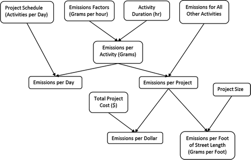
Emissions factors are multiplied by the amount of time that the equipment was used and by its horsepower to obtain the total emissions for each activity. The total emissions for the project were determined by summing the total emissions for each activity. The total quantity of emissions was then used to calculate productivity emissions rate factors (emissions per dollar and emissions per foot of street length) by dividing total emissions by the total length of the street constructed and total emissions by the total cost of the project as calculated using RS Means. If desired, it is also easily possible to determine emissions per day. Figure 1 is a visual representation of these calculations steps. In Figure 1, the five bubbles leading into the left side of ‘Emissions per project’ bubble refer to an individual activity. These steps are undertaken for all of the other project activities as well. We used the bubble to the upper right of the ‘Emissions per project’ bubble to represent this.

Figure 1. Diagram of emissions calculation steps.

The cost emissions rate is an important early stage emissions indicator, enabling an unrefined emissions estimate to be obtained for a project based solely on knowing its preliminary cost. This is important because these totals represent the project’s overall environmental impact. Over time, such a preliminary estimate can be more precisely determined as more is learned about the details of the project such as the actual construction activities to be undertaken and details about the composition of the actual construction equipment fleet to be used.

Results

This section presents the emissions results for each entire project as well as for individual project activities. All four projects are compared. It is important to note that street construction projects have activities that include heavy equipment use which tend to produce emissions throughout the entire project.

Project CO₂ emissions

While our entire study encompassed six pollutants, we are presenting results here only for CO₂ because this pollutant is prevalent in previous literature and because CO₂ is linked to climate change. The total daily project emissions for CO₂ for the four projects are presented in Figures 2–5. The profiles for all the other pollutants follow a similar shape with different magnitudes of daily total emissions. These are discussed in later sections.

Figure 2. CO₂ emissions per day for the Little Street project.

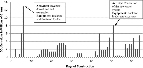
Figure 3. CO₂ emissions per day for the West Burkhead project.

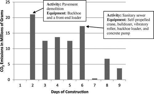
Figure 4. CO₂ emissions per day for the Sutton Place project (Phase 1).

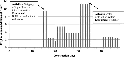
Figure 5. CO₂ emissions per day for the Sutton Place project (Phase 2).

The CO₂ emissions distribution for the Little Street project is presented on Figure 2. The figure shows a high peak on day six of the construction project. The activities for day six included pavement demolition and the excavation needed during demolition and required the use of a backhoe and a front-end loader. The second-highest quantity of emissions occurred on day 51 and corresponded with work for the connection of the new water system to the existing metres and the installation of storm water piping under the street. The crew for these activities included a backhoe loader and an excavator and consisted of trenching, backfilling and other excavation activities. The total project CO₂ emissions were approximately 112 million grams and the average emissions per day were 1.7 million grams.

The CO₂ emissions distribution for the West Burkhead project is presented on Figure 3. This was an extremely short project. The figure shows a high peak on the second day of construction when the contractor was demolishing the existing street. The crews for these activities required the use of a backhoe and a front-end loader working to demolish the street and load the material into dump trucks for disposal. The sanitary sewer was either abandoned or demolished and replaced during day six, resulting on another, but smaller, peak. The equipment utilised by the crews for these activities were: self-propelled crane, bulldozer, vibratory roller, backhoe loader and concrete pump. The total project CO₂ emissions were approximately 88 million grams and the average emissions per day were 9.7 million grams.

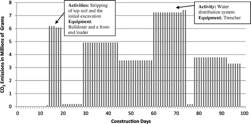
Figures 4 and 5 show the CO₂ emissions for the two phases of the Sutton Place project. The distributions of emissions were very similar in shape because both phases were comprised of the same activities with different quantities. The highest emissions production occurred during the installation of the water distribution system that included the use of a trencher. The water system installation occurred on days 32–36 for Phase 1 and days 61–75 for Phase 2. The second-highest emissions quantities correspond to the stripping of top soil and the initial excavation. The crews for these excavation activities included a bulldozer and a front-end loader. The stripping and excavation activities occurred during days 16 and 17 on Phase 1 and days 15–29 on Phase 2. For Phase 1, the total project CO₂ emissions were approximately 147 million grams and the average emissions per day were 3 million grams. For Phase 2, the total project CO₂ emissions were approximately 356 million grams and the average emissions per day were 3.5 million grams.

Other pollutants

To illustrate the collective impact of all six of the pollutants we introduce Figure 6, which presents the emissions from the Little Street project study. These emissions are presented as a percentage of total emissions by days of construction. There were two distinctive groups of pollutants. HC, CO and PM all start at a higher percentage than CO₂, SO₂ and NO_x. The basic difference between these two groups was the front-end loader (used for the demolition activities) which tends to produce more HC, CO and PM. The bulldozer and rollers tend to produce more of the other three pollutants and were used more often, for longer periods, and at a later time in the project than the front-end loader was. As a result, the percentage of total emissions for HC, CO and PM that is produced at the beginning of the project is much higher than the percentage of the other pollutants. The emissions for CO₂ and SO₂ (the bottom two overlapping lines) have nearly identical shapes because both factors are directly derived from fuel use.

Figure 6. Cumulative emissions for all pollutants for Little Street project.

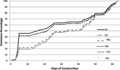
The graph in Figure 6 also presents three slopes for emissions production. A large quantity of emissions is produced at the beginning of the project resulting in an almost vertical slope up to day 5. From day 6 to 42, the emissions production is relatively constant resulting in a gently increasing slope. From day 43 to 64, the emissions production increases resulting on a steeper slope. The graph shows that by day 42, two-thirds of the duration of the project, 66% of HC, PM and CO was produced as well as 50% of NO_x, CO₂ and SO₂. In the case of this project and the others, the majority of the emissions were produced at the beginning and at the end of the project.

The configuration presented in Figure 6 is opposite to the lazy S graphs that are often observed in other construction related data. An example of this type of graph is a typical cash flow curve. The cash flow at the beginning of a project is slow, resulting in a gentler slope. Later during the project, the cash flow increases, resulting on a more pronounced slope during the middle of the project. At the end of the project, the cash flow again decreases, resulting in a gentler slope. Emissions production seems to have a different pattern to what is normally expected for construction resources.

The other three projects that were studied had similar profiles for the six pollutants. For these projects the CO and PM lines are again extremely close to each other. This also holds true for the CO₂ and SO₂ lines.

Activity emissions

The emissions profiles for all four projects show that differing levels of emissions were produced over time for the entire duration of the project. The majority of all of the activities that are required to complete a transportation project include the use of non-road diesel-powered equipment.

Table 4 shows the per cent of total emissions for each project activity for the projects that have a demolition activity (and for each pollutant) as well as the average percentage of emissions for each pollutant. For both Little Street and West Burkhead, demolition was the activity that produced the largest amount of HC, CO and PM emissions. Earthwork produced similar emissions amounts. The high emissions quantities for the peak activities of demolition and earthwork are directly linked to the equipment used and the high emissions factors for that equipment. For the projects that did not have a demolition activity (Sutton Place Phases 1 and 2) earthwork was the activity with the highest quantity of emissions for both projects and for all the pollutants.

Table 4. Per cent of emissions for each activity for projects with demolition.

Project	Pollutant	Per cent of total emissions per activity
		Demolition	Earthwork	Utility installation	Paving	Other
Little Street	HC	49	19	11	14	7
	CO	45	25	8	16	6
	NOx	22	30	21	17	11
	PM	45	23	10	16	6
	CO2	19	33	20	19	10
	SO2	19	33	20	19	10
West Burkhead	HC	40	37	9	7	7
	CO	37	41	6	9	7
	NOx	16	54	11	9	9
	PM	35	43	7	8	7
	CO2	14	60	10	10	8
	SO2	14	60	10	10	8
Average	HC	45	28	10	11	7
	CO	41	33	7	13	7
	NOx	19	42	16	13	10
	PM	40	33	9	12	7
	CO2	17	47	15	15	9
	SO2	17	47	15	15	9

Table 4 provides the quantification of our research results, which could be made available to the research community. We have also included Figure 7 to illustrate the relative comparison between the different pollutant types and between the two projects with demolition. This chart allows for a quick comparison in terms of per cent emissions.

Figure 7. Visual representation of the per cent of emissions for each activity for projects with demolition.

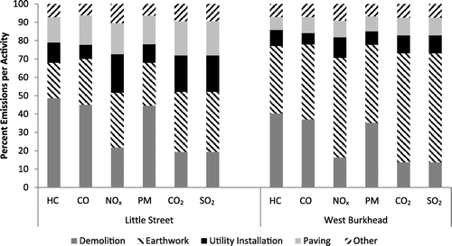
An important factor affecting total project emissions is the amount of work that has to be completed over time. For example, demolition and earthmoving activities not only utilised highly polluting equipment (with high emissions factors) but they also required the movement of a large quantity of the material in a small amount of time. Demolition for Little Street was completed in two days and for West Burkhead in one day.

Demolition and earthwork activities both utilise front-end loaders. These have a large emissions factor for HC, CO and PM. The bulldozer and trenchers used for the earthwork (and other later activities) emit more NO_x, CO₂ and SO₂. This is reflected on the emissions percentages shown in Table 3.

Emissions by equipment type

The analysis of emissions per activity showed that demolition and earthwork are the most polluting type of activity. The main equipment types used for these activities were backhoes, front-end loaders, bulldozers and trenchers. Table 2 showed that front-end loaders and backhoes are the equipment with the largest emissions factors for HC, CO, NO_x and PM from the NONROAD model.

Table 5 shows the percentage of emissions produced by each item of equipment for each pollutant. Front-end-loaders are the major contributor of HC, CO, NO_x and PM emissions while trenchers produced the highest average emissions for CO₂, and SO₂. As before, Figure 8 presents these data using a stacked bar chart.

Table 5. Per cent emissions by equipment type for the projects.

Project	Pollutant	Per cent emissions per equipment type
		FE Loader	Bulldozer	Roller	Trencher	Backhoe	Crane	Excavator	Grader	Other
Little Street	HC	41	10	12	NA	13	8	0	2	15
	CO	37	13	15	NA	13	5	1	2	16
	NOx	17	18	16	NA	8	17	1	3	24
	PM	37	12	15	NA	13	7	1	2	16
	CO2	15	19	18	NA	7	16	1	3	25
	SO2	15	19	18	NA	7	16	1	3	25
West Burkhead	HC	28	5	6	NA	18	5	14	16	24
	CO	25	6	8	NA	17	3	16	16	25
	NOx	10	7	7	NA	9	10	21	24	36
	PM	24	5	7	NA	16	4	17	17	26
	CO2	8	7	7	NA	6	10	24	26	37
	SO2	8	7	7	NA	7	8	24	26	37
Sutton Place Phase 1	HC	45	6	7	31	NA	0	5	2	4
	CO	37	8	8	38	NA	0	5	2	4
	NOx	21	12	10	38	NA	1	10	5	8
	PM	38	7	8	35	NA	0	6	3	5
	CO2	17	13	11	38	NA	1	12	5	9
	SO2	17	13	11	38	NA	1	12	5	9
Sutton Place Phase 2	HC	35	9	10	29	NA	0	8	5	9
	CO	28	10	12	35	NA	0	8	4	8
	NOx	14	15	14	31	NA	0	13	8	13
	PM	29	9	12	32	NA	0	9	5	9
	CO2	11	15	14	30	NA	0	14	9	14
	SO2	11	15	14	30	NA	0	14	9	14

Note: NA signifies that the specified equipment was not used on that project.

Figure 8. Visual representation of the per cent emissions by equipment type for the projects.

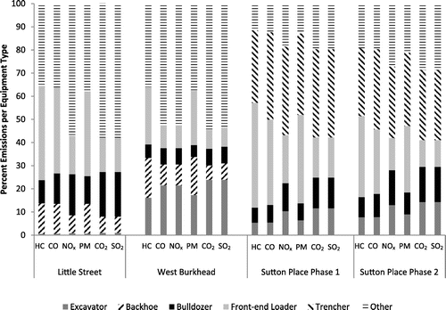
The type of equipment used for each project was different. Trenchers were not used for Little Street and West Burkhead. Sutton Place Phase 1 and Sutton Place Phase 2 did not use backhoes. Table 4 clearly shows that front-end loaders and trenchers are the two equipment types with the largest effect on pollutant emissions followed by excavators and bulldozers.

Differences between the four street projects

It is interesting to compare the results for the four street projects because they had different characteristics that produced different emissions profiles.

Both the Little Street and West Burkhead projects were rehabilitations that included removing the existing street and removing and reinstalling the utility system. The Sutton Place project was a new street for a subdivision and included only the installation of utilities and required no demolition and removal. Tables 3 and 4 showed the emissions per activity that reflect the different distribution of work per project.

The differences between the four projects’ characteristics account for the differences between their emissions per activity. However, a comparison of emissions by per cent complete for the four projects highlights similarities. Figure 9 shows the cumulative emissions over time for all four street projects. For all the street projects, the first few days of construction were used for mobilisation and preparation without the use of non-road equipment. This is reflected in the low emissions production rate shown. After that, the first activity included the preparation of the entire area of construction (demolition and earthwork) producing a sharp initial jump in emissions. Various items of equipment were continuously used, producing different but nearly continuous amounts of emissions each day and resulting in similar emissions graphs for all the projects.

Figure 9. Comparison of cumulative CO₂ as per cent for street projects.

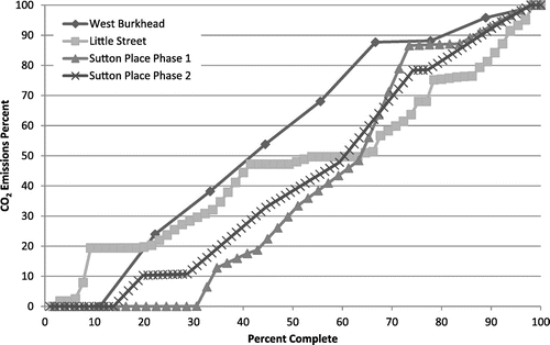
Figure 9 also shows that even when all the projects have a similar behaviour over time, the two projects that require demolition and repaving (West Burkhead and Little Street), have higher emissions at the beginning of the project. The two new construction projects (Sutton Place 1 and Sutton Place 2) have a slower production rate of emissions at the beginning of the project.

For the Little Street and West Burkhead projects, half of the emissions were produced before the projects were 40% completed. When the West Burkhead project was half way completed, two-thirds of the emissions had already been produced. For Sutton Place, 30 and 37% of the emissions for Phases 1 and 2, respectively, were produced at the midpoint of the project.

Table 6 shows the emissions per thousand dollars and per foot of street length for the four street projects. The rates were calculated using the total cost resulting from the RS Means information. There were not major differences in the rates between the projects, which should build confidence in the use of the averages.

Table 6. Emissions metrics for the street construction projects.

Metric	Pollutant	Average Street	Little Street	West Burkhead	Sutton Place Phase 1	Sutton Place Phase 2
Grams per thousand dollars	HC	97	95	109	106	80
	CO	747	680	787	865	656
	NOx	814	791	998	797	670
	PM	3	3	3	3	2
	CO2	680,000	629,000	845,000	673,000	572,000
	SO2	119	110	148	118	100
Grams per foot of street length	HC	17	21	17	18	13
	CO	144	164	135	162	115
	NOx	157	190	165	154	120
	PM	0.5	0.57	0.5	1	0
	CO2	1.62E+05	1.88E+05	1.76E+05	1.59E+05	1.27E+05
	SO2	28	33	31	28	22

Conclusions

The fundamental questions addressed in this paper were how to quantify (and thus determine) the emissions produced for the construction of street and utility transportation construction projects, what factors resulted in higher or lower emissions (and how do these change over time) and how do different project types compare with respect to emissions production? The objective of this work was to provide a methodology to estimate emissions from street and utility infrastructure projects. No similar work had previously been done.

Our finding was that the available data sources did prove to be adequate to support the estimates generated herein. The methodology was able to produce adequate results. Thus, engineers and contractors could use them for emissions estimates for street and utility projects. As a further refinement they could enter their own actual equipment fleet into the model to obtain emissions estimates tailored to both their project and to their equipment.

Related to the equipment fleet is an important note relative to the use of RS Means. We found that RS Means provided a generic equipment fleet composition that naturally differs from the actual fleet composition owned by the contractors. However, this did not result in a total emission production difference thus indicating that a RS Means estimate could be used when actual equipment data is unavailable, such as during early project planning stages.

The four street construction projects showed similar profiles of emissions. All four projects experienced a period without emissions at the beginning of the project followed by a short period with very high emissions production. After that, emissions were uniformly produced at a relatively steady rate throughout the rest of the project, with perhaps one more peak during the second half of the period. This uniform emissions production occurred, in part, because street construction requires the use of non-road equipment for the majority of the activities. As a result, it is clear that the profile is quite similar for the street projects. These results holds true for all pollutants.

This study showed that demolition and earthwork have a significant impact on the emissions produced during street construction. Those interested in emissions should pay close attention to these activities because changes in activity duration and productivity could have a significant impact on total project emissions. These activities would be particularly important to maintain and control if emissions regulations are put in place to regulate daily emissions peaks.

The equipment types for the four street construction project with the greatest influence on emissions were backhoes, front-end loaders, bulldozers and trenchers. These types of equipment have high NONROAD model emissions factors. However, because of their versatility, these items of equipment will continue to be used for a wide variety of construction activities and thus, will continue to be large emissions producers.

When examining the emissions profiles for all the pollutants we observed that HC, CO and PM were produced at higher rates at the beginning of the project while CO₂, SO₂ and NO_x tended to be produced later. Furthermore, these two groupings of the six pollutants exhibit similar characteristics and trend together tightly. This could have implications for those trying to regulate particular types of pollutants.

It was also observed that the graph of cumulative emissions production during the project has a different configuration than the one typically seen for construction factors. The graph does not present the lazy-S shape but more of a lazy-Z shape. The graph shows a large rate of emissions at the beginning of the project, a slower rate during the middle of the project and another larger rate at the end of the project.

Results also showed that some activities have a larger contribution of emissions for each project. Future construction professionals and regulators can use this knowledge to concentrate their pollution reduction efforts on the construction activities that have the largest impact on total emissions.

Comparisons between the different projects were made using measures of emissions per dollar of construction cost. These factors can be used in the future to develop estimates for construction projects during their planning or early construction phases. Being able to accurately estimate emissions in an early planning or design stage will be beneficial for addressing future environmental and emissions regulations and in achieving desired pollution reductions.

Future work

The work presented herein utilised both contractor and R. S. Means data to estimate the total quantity of emissions for four street construction projects using EPA emissions factors for typical construction equipment types and sizes. The work does not, however, account for the fact that any given contractor has a limited availability of equipment in his fleet for use on his construction projects. Future work should include the estimating of project emissions based on the specific equipment type and tier actually used on site during the project. Hopefully, data can be obtained from contractors who maintain a detailed equipment use record that includes daily hours of operation and fuel use as well as basic specifications about the equipment used.

Future work should also be directed at determining the effects of different equipment characteristics on emissions factors. Having a better understanding of the effects of equipment type, engine size and engine tier on the emissions can help contractors to make decisions on equipment usage to comply with future regulations. It can also aid in their selection of new equipment purchases. Additional work should also be done to determine the effect of engine tier on emissions. Calculating total emissions using equipment of different tier can help to determine the difference on emissions and assess the effect of the regulations.

In the future, different types of projects should be analysed to see how their emissions profiles compare to projects analysed to this point. This could include residential buildings, commercial buildings, high-rise buildings and various types of transportation projects beside streets. The results presented here found clear similarities between street construction projects. A larger numbers of studies need to be undertaken. A larger emissions inventory needs to be assembled to better establish the generalisability of the results presented in studies such as this one.

Only non-road construction equipment was studied herein. Future studies should obtain detailed estimates of pollutants for on-road vehicles such as dump trucks, flatbed trucks and concrete mixer trucks. The EPA NONROAD model used here only offers emissions factors for equipment that does not travel on the road. The EPA also developed a model to estimate emissions from on-road vehicles called MOVES. However, the categories used by this model to determine emissions do not include ones that correspond to construction vehicles moving on the road. Future studies should be completed to find the best alternative for these emissions factors.

This paper focused on emissions from non-road heavy-duty diesel-powered equipment that is used on construction sites. The pollutants studied were the exhaust pollutants from construction equipment; we did not include other emissions related to a construction projects such as fugitive particulate matter (e.g. from dust). Additional work should be done to assess the effects of all the emissions associated with the use of construction equipment on the construction site. This estimation would help to assess the effect of construction activities on the workers, operators and the community.

Useful measures of emissions are critical for the proper assessment of their impact in the Architecture-Engineering-Construction and infrastructure markets. We presented measures of emissions per dollar and per foot of street length because these measures are clearly useful at all project stages and can be used for long-term planning as well. Of course, additional research is needed to assess the variability of the emissions per dollar and per foot of street length metrics on projects of varying size and cost. A variety of other measures should be considered, studied and quantified as well.

Finally, more research needs to be done to determine the effect of possible future regulations on emissions and the resulting productivity of construction activities. New and stricter regulation could have a significant impact on the construction methods currently used by contractors. Having an accurate estimating model (and taking into consideration the unique characteristics of construction work) may enable government agencies to develop regulations that will help to reduce air pollution from construction projects. Construction professionals could themselves use more accurate estimates to make decisions on what is the most efficient way to reduce emissions without negatively affecting productivity.

Disclosure statement

No potential conflict of interest was reported by the authors.

Notes on contributors

Ingrid Arocho is an Assistant Professor at the School of Civil and Construction Engineering at Oregon State University. Arocho's research interests include construction equipment management, pollution production during construction activities and construction methods improvement to reduce environmental impact.

William Rasdorf is a Professor at the Department of Civil, Construction and Environmental Engineering at North Carolina State University. Rasdorf's research interests include engineering databases and infomation processing, automated representation, computer -aided design and geometric and spatial modelling and analysis in engineering.

Joseph Hummer is a staff engineer at the Mobility and Safety Division at North Carolina Department of Transportation. Hummer's research interests include the design and operation of unconventional intersections and interchanges, traffic control devices and collision prediction models.

Phil Lewis is an Assistant Professor at the School of Civil and Environmental Engineering at Oklahoma State Univesity. Lewis' reserach interests include the environmental impacts of construction and sustainable construction.

References

- Baouendi, R., R. Zmeureanu, and B. Bradley. 2005. “Energy and Emission Estimator: A Prototype Tool for Designing Canadian Houses.” Journal of Architectural Engineering, American Society of Civil Engineers 11 (2): 50–59.
- Bilec, M., R. Ries, and H. S. Mathews. 2010. “Life-Cycle Assessment Modeling of Construction Processes for Buildings.” Journal of Infrastructure Systems, American Society of Civil Engineers 16 (3): 199–205.
- EPA. 2005. User’s Guide for the Final NONROAD2005 Model. EPA-420-R-05-013. Ann Arbor, MI: U.S. Environmental Protections Agency, Office of Transportation and Air Quality.
- EPA. 2008. Quantifying Greenhouse Gas Emissions from Key Industrial Sectors in the United States (Working Draft). Washington, DC: US Environmental Protection Agency, Sector Strategies Program.
- EPA. 2009. Potential for Reducing Greenhouse Gas Emissions in the Construction Sector. Washington, DC: US Environmental Protection Agency, Sector Strategies Program. Accessed September 7, 2014. http://www.epa.gov/sectors/pdf/construction-sector-report.pdf
- EPA. 2010a. Exhaust and Crankcase Emissions Factors for Nonroad Engine Modeling – Compression Ignition. EPA-420-R-10-018. Ann Arbor, MI: U.S. Environmental Protection Agency, Office of Transportation and Air Quality.
- EPA. 2010b. Median Life, Annual Activity, and Load Factor Values for Nonroad Engine Emissions Modeling. EPA-420-R-10-016. Ann Arbor, MI: U.S. Environmental Protection Agency, Office of Transportation and Air Quality.
- EPA. 2013. National Ambient Air Quality Standards (NAAQS). Washington, DC: US Environmental Protection Agency. Accessed September 7, 2014. http://www.epa.gov/air/criteria.html
- Guggemos, A. A., and A. Horvath. 2006. “Decision-Support Tool for Assessing the Environmental Effects of Constructing Commercial Buildings.” Journal of Architectural Engineering, American Society of Civil Engineers 12 (4): 187–195.
- Junnila, S., A. Horvath, and A. A. Guggemos. 2006. “Life-Cycle Assessment of Office Buildings in Europe and the United States.” Journal of Infrastructure Systems, American Society of Civil Engineers. 12 (1): 10–17.
- Kim, B., H. Lee, H. Park, and H. Kim. 2012. “Greenhouse Gas Emissions from Onsite Equipment Usage in Road Construction.” Journal of Construction Engineering and Management, American Society of Civil Engineers 138 (8): 982–990.
- Lee, J. C., T. B. Edil, C. H. Benson, and J. M. Tinjum. 2011. “Evaluation of Variables Affecting Sustainable Highway Design with BE2ST-in-Highways System.” Transportation Research Record: Journal of the Transportation Research Board 2233: 178–186.
- Lewis, P., H. C. Frey, and W. Rasdorf. 2009. “Development and Use of Emissions Inventories for Construction Vehicles.” Transportation Research Record: Journal of the Transportation Research Board 2123: 46–53.
- Lewis, P., W. Rasdorf, C. Frey, S. Pang, and K. Kim. 2009. “Requirements and Incentives for Reducing Construction Vehicle Emissions and Comparison of Nonroad Diesel Engine Emissions Data Sources.” Journal of Construction Engineering and Management, American Society of Civil Engineers 135 (5): 341–351.
- Lewis, P., W. Rasdorf, H. C. Frey, and M. Leming. 2012. “Effects of Engine Idling on National Ambient Air Quality Standards Criteria Pollutant Emissions from Nonroad Diesel Construction Equipment.” Transportation Research Record: Journal of the Transportation Research Board 2270: 67–75.
- Marshall, S. K., W. Rasdorf, P. Lewis, and H. C. Frey. 2012. “A Methodology for Estimating Emissions Inventories for Commercial Building Projects.” Journal of Architectural Engineering, American Society of Civil Engineers 18 (3): 251–260.
- Means, R. S. 2013. Building Construction Cost Data. Kinston, MA: R. S. Means Company. http://www.rsmeansonline.com/.
- Sharrard, A., H. S. Matthews, and R. J. Ries. 2008. “Estimating Construction Project Environmental Effects Using an Input-output-based Hybrid Life-cycle Assessment Model.” Journal of Infrastructure Systems 14 (4): 327–336.10.1061/(ASCE)1076-0342(2008)14:4(327)
- Tatari, O., and M. Kucukvar. 2012. “Sustainability Assessment of U.S. Construction Sector: Ecosystems Perspective.” Journal of Construction Engineering and Management, American Society of Civil Engineers 138 (8): 918–922.