Impact of incorporating customer preference in sustainable remanufacturing of commercial returns

Abstract

This paper investigates optimum production parameters for a reverse supply chain for manufacturing of primary products and remanufacturing of commercial returns (products returned by customers for refund or exchange). The market for the product consists of two categories, the primary and remanufactured products. The demands for these markets are independent and considered to be random variables following a normal distribution function. The approach presented in this work differs from many previously published works because the acceptability of products varies among customers. The interaction between the designed quality and variable customers’ preferences determines the likelihood of a product being returned. Two major decision variables targeted in this study are the production cycle time and the targeted quality for production of parts used in the product. Through an analytical formulation and numerical examples, a relationship between the total profit of the system and the two decision variables is developed and optimised. The analysis demonstrates that the total profit of the hybrid system could be increased significantly by targeting the optimum targeted (not necessarily the highest) values for quality of parts and the optimum cycle length. And this objective could be accomplished with significant gain with respect to sustainability and waste reduction.

Keywords:

• Remanufacturing
• sustainability
• optimisation
• reverse supply chain
• customer preference function

1. Introduction

Nowadays, product recovery is drawing much attention due to the increased environmental concerns, awareness of natural resource limitations in the world, and economic advantage of recycling materials. The objective of product recycling is recovering as much of the economic (and ecological) value as reasonably possible, thereby reducing the ultimate quantities of waste.

Remanufacturing of products from parts recovered from returned units represents a huge profit potential for companies. Based on a report by Gallagher, Mitchke, and Rogers (2005), the supply of aftermarket products is a $400 billion business. Surprisingly, the volume of research on treatment of these returns has not yet matched the magnitude of the complexities and intricacies involved. As it is explained later on this research, product development and supply chain design can highly influence the revenue of the aftermarket products and sustainability concerns.

The motivation behind this research is to formulate a realistic production inventory model for a combined manufacturing/remanufacturing system supplying a mixed demand for primary, defined as new products made of new parts, and remanufactured products produced using parts from returned products. In other words, it is assumed that the total demand can be broken down to a demand for primary products, D_Ni, and one for aftermarket products, D_Ri. The system is then set up to supply both demands.

Numerous remanufacturing models have been developed by researchers and are available in the existing literature (Dobos 2003; Fleischmann, van Nunen, and Gräve 2003; Gu and Tagaras 2014; Hsueh 2011; Poles 2013). Relatively a small portion of these works have concentrated on new products that are returned, taking advantage of generous return policies Original Equipment Manufacturer (OEMs) offer to customers (Blackburn et al. 2004; Guide et al. 2006). A customer might return a new (recently bought) product for a variety of different reasons, for instance, the product being defective, the performance of the product not meeting the customer’s expectance, or even finding a lower price on the same product from a different retailer. Davey et al. (2005) extensively studied such a case for printers sold by Hewlett-Packard Company.

Among the few mentioned research that address the issue of new product returns, none has considered variations among customers’ behaviours with respect to returning a product. A product that functions properly but has some minor flaws may be returned by some customers while others would be happy to keep. In other words, the level of quality tolerance varies among customers. Therefore, inclusion of a customer quality tolerance function reflects a more realistic estimation of the product return rate thus providing better opportunities for product and process designs. Incorporation of a realistic customer quality tolerance function for a manufacturer requires extensive research for the specific demographic of which the products are being sold to. Nonetheless, authors believe that performing such complex research is absolutely crucial for each manufacturer since it affects the outcome of the presented model significantly.

Hence, incorporating a customer quality tolerance function in consideration of decision policies (referring to the main variables that affect the model outcome) in a manufacturing/remanufacturing system is one of the major contributions of this paper. Two decision policies incorporated in this paper are the target quality of parts used to manufacture primary products and the length of each remanufacturing cycle. Additional characteristics of the system include:

•	There are N equal cycles during the study period T, denoted by cycle 1, 2, …, i, …, N. The demand for primary and aftermarket products in each cycle are random variables following a normal distribution with pre-determined parameters.
•	The rate of returned items collected from the market depends on the production quality and the acceptability of products by customers. A customer preference function has been defined that divides customers into several categories with different levels of tolerance for defects. The interaction between the targeted quality of parts when producing the primary products and this function determines the return rate of the primary products. Targeting higher parts quality results in lower return rates and higher production costs and therefore there are fewer products available to remanufacture and satisfy the aftermarket demand. Targeting lower parts quality, however, results in an excessive number of returns. Although, in this case the aftermarket demand is satisfied, the increased remanufacturing cost lowers the net profit.
•	The system is in steady state, meaning that in the beginning of the first cycle there is already a supply of returned products available to start remanufacturing simultaneously with manufacturing of primary products.
•	The production rate of primary products and remanufacturing rate of commercial returns are known and, for simplicity purposes, are assumed to be the same for all production cycles. In addition, these rates are assumed to be greater than the demand rates for primary and remanufactured products.

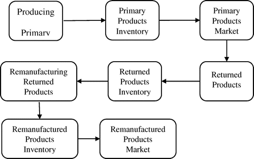
Figure 1 shows a flow chart for this supply chain model.

Figure 1. Product flow chart of the system.

This paper is organised as follows. Section 2 reviews the literature on related reverse logistics. Section 3 formulates the problem analytically. Section 4 presents several numerical examples to review the application of the proposed model and finally Section 5 outlines the conclusions.

2. Literature review

The design of optimal supply chains has been long studied in the literature. Moreover, inventory planning for remanufacturing is investigated by several authors in the literature. Richter and Sombrutzki (2000) used a deterministic model where the main aim was to investigate the effect of returns on the optimal order quantity. The stochastic version of the problem is studied by van der Laan, Salomon, and Dekker (1999). In that study, manufacturing and remanufacturing operations are considered as single stage operations; therefore, the effect of relative values of new and used products at different operations is not investigated in detail.

Poles (2013) developed a system dynamics simulation model of a production and inventory system focusing on the remanufacturing process. The main factors considered for the simulation of the model were inventory coverage, total system capacity, and remanufacturing and production lead times. They concluded that the total system cost increases more rapidly if higher capacity is allocated to the remanufacturing than the production activity. Their results suggest that it is advisable to increase the level of remanufacturable returns and reduce remanufacturing lead times in order to reach higher efficiency in the remanufacturing process.

Hsueh (2011) investigated inventory control policies for manufacturing/remanufacturing by considering different product life cycle phases. Vercraene, Gayon, and Flapper (2014) studied the coordination of manufacturing, remanufacturing and returns acceptance in a hybrid manufacturing/remanufacturing system and proposed several heuristic control rules. Moreover, Hsueh (2015) studied the optimal inventory and pricing policies in a decentralized production/remanufacturing system with multiple refurbished components. It was proposed that in a deterministic problem, the manufacturer can influence the product demands and the quantity of returned end-of-use products.

Shen, Coullard, and Daskin (2003) initiated an interesting line of research by integrating inventory decisions into strategic facility location designs. In addition, in their inventory control policy, a fixed quantity is ordered from the supplier once the inventory level falls below a reorder point. The total number of shipments per year was considered as a decision variable.

Among reverse logistics literature, Fleischmann, van Nunen, and Gräve (2003) studied reverse supply chain of IBM spare parts. Their inventory control model and simulation showed that reverse logistics present significant savings over procurement costs. Moreover, Fleischmann and Minner (2004) reviewed the different inventory control models in the reverse logistics supply chains and concluded that there is a need for integration of inventory control decisions with the other business functions in closed-loop supply chains.

Gu and Tagaras (2014) considered a reverse supply chain comprising two independent companies: the collector and the remanufacturer. The collector is responsible for sorting the collected used products and then transporting the ‘remanufacturable’ items to the remanufacturer. They have showed that under certain conditions, the remanufacturer should allow the collector to transport more ‘remanufacturables’ than the order quantity.

Dobos (2003) found optimal inventory policies in a reverse logistics system with special structure while assuming that the demand is a known function in a given planning horizon and the return rate of used items is a given function. The demand is satisfied from the first store, where the manufactured and remanufactured items are stored. The returned products are collected in the second store and then remanufactured or disposed of. Dobos (2003) minimised the sum of the holding costs in the stores and costs of the manufacturing, remanufacturing and disposal.

Kiesmüller and van der Laan (2001) investigated an inventory model for a single reusable product, where the random return depends on the demand based on the assumption that the selling quantity is approximately equal to the demand. The results show that it is necessary to consider the dependence between the demand process and the return process. Dobos and Richter (2004) investigated a production/recycling system where customer demand and return rates are deterministic and stationary. They consider the Economic Order Quantity (EOQ) environment with recovery and define return rate as a fraction of the constant demand rate.

Alinovi, Bottani, and Montanari (2012) focused on mixed manufacturing/remanufacturing systems, where manufacturing of new items integrates product reuse or remanufacturing. Their study ultimately provides a framework for practitioners to establish EOQ policies in reverse logistics contexts and to evaluate the opportunity of establishing a return policy. Moreover, a recovery system for perishable items is introduced and developed by Feng, Zhang, and Tang (2013) considering production and remanufacturing capacity constraints. The system consists of two inventories, one for serviceable items and the other for returned and recoverable items. The optimal control model is established to minimise the total cost. It is shown that the continuous-time dynamic optimal policy is significantly better than static optimal policy that does not vary with time.

Another factor that has been investigated in the presented research is the impact of targeted quality of parts used for manufacturing the primary products. Ardeshirilajimi and Azadivar (2015b) considered the time value of money using two key decision policies affecting the performance of a reverse supply chain system, the target quality for components used in the primary product and duration of the time returned products are accumulated before they are remanufactured, to maximise the total profit. Moreover, Ardeshirilajimi and Azadivar (2015a) studied various aspects influencing the efficiency of the remanufacturing activities with the main objective of maximising the net profit for the manufacturer focusing on the key decision policy of the targeted quality of components.

The added value of this research to the existing literature is twofold. First, the rate of return for product is not only as a function of product quality, but is also affected by a variable customer preference demonstrated by a customer preference function. This is an innovative idea in order to help the manufacturer better estimate the return rate for their products. Second, inventory levels for primary, returned and remanufactured products are controlled by quality of parts used in manufacturing primary products and the manufacturing/remanufacturing production cycles.

3. Proposed model

This section presents the assumptions, in Table 1, and notations, in Table 2, used throughout this article. Then the model is presented.

Table 1. Assumptions.

(1)	There are two independent stochastic demands for primary products, DNi, and remanufactured products, DRi in each cycle. The means and standard deviations of these two demands are assumed to be known
(2)	The return rate for remanufactured products is negligible
(3)	All production cycles have the same duration
(4)	Returned products stay in the returned products inventory, at least until the end of the cycle they were returned in, before they are used for remanufacturing
(5)	The manufacturing rate is constant and is greater than the demand rate for primary products
(6)	Remanufacturing rate is constant and is greater than the demand rate for remanufactured products

Table 2. Notations.

i	Cycle number
DNi	Demand for the primary products in the ith cycle
DRi	Demand for the remanufactured products in the ith cycle
T	Study period
N	Number of cycles in the study period
PP	Production rate of primary products
RR	Remanufacturing rate of returned products
R	Return rate for primary products
tc	Time period for a cycle
tpi	Duration of production in the ith cycle
Ini(t)	Inventory level for primary products at the ith cycle
ICNi	Total Inventory costs for primary products at the ith cycle
A1	Inventory carrying cost of a unit of primary product per unit time
PCNi	Total production cost for primary products at the ith cycle
A3, A4	Parameters defining the economy of scale for production costs
A2	Set-up costs for producing primary products
Sn	Selling price per unit of primary products
PNi	Total profit from selling the primary products in the ith cycle
Iui(t)	Inventory level for returned products at the ith cycle
ISui	Returned products inventory level at the beginning of the ith cycle
IEui	Returned products inventory level at the end of the ith cycle
ICUi	Inventory costs for the returned products at the ith cycle
IRi(t)	Inventory level for remanufactured products at the ith cycle
ISRi	Remanufactured products inventory level at the beginning of the ith cycle
IERi	Remanufactured products inventory level at the end of the ith cycle
ICRi	Total Inventory costs for remanufactured products in the ith cycle
A5	Inventory carrying cost of a unit of returned product per unit time
A6	Inventory carrying cost of a unit of remanufactured product per unit time
RCUi	Remanufacturing costs for returned products in the ith cycle
Sr	Selling price per unit of remanufactured products
PRi	Total profit from selling remanufactured product in the ith cycle
TP	Total profit during study period
S0, S1, S2, S3, S4	Parameters defining customer satisfaction function
n	Number of components in a product
p	Targeted quality of parts defined as the defective rate in the production process
A7, A8	Parameters defining the economy of scale for disassembly costs of returned products
A9, A10	Parameters defining the economy of scale for reassembly costs of returned products
TD	Total defective components in a single batch of returned products
A11	Cost per unit of a new component

3.1. Assumptions and Notations

See Tables 1 and 2.

3.2. The model

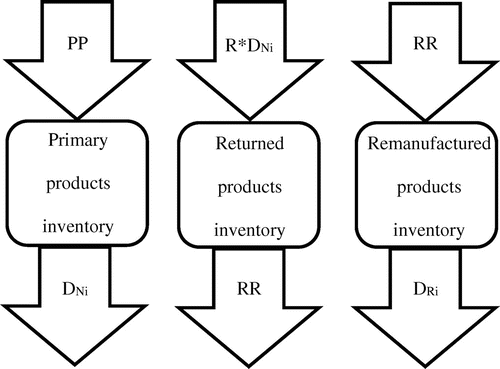
We assume three different inventory systems; one for primary, one for returned and one for remanufactured products. The company starts producing primary products at a constant rate at the beginning of each cycle, and continues until the inventory for primary products is enough to satisfy the demand in that cycle, designated by D_Ni. In addition, the demand for remanufactured products in each cycle, designated by D_Ri, is satisfied by products built from returned products inventory.

These inventories are shown in Figure 2.

Figure 2. Three inventory systems product flow.

The assumptions for the inventory units are:

(1)	Primary products inventory: In every cycle, the manufacturer produces and supplies primary products to this inventory with the rate of PP.
(2)	Returned products inventory: The return rate for remanufactured products is assumed to be zero. Therefore, the only input to the returned products inventory comes from customers who return primary products. The logic behind this assumption is the fact that the volume of these returns is of the second order of the fraction return of primary products which by itself is within a few percentage points. The simplification in modelling and analysis due to this assumption could easily outweigh its negligible impact on results. This assumption could also be valid if remanufactured products are not covered by return warranty. Therefore, representing return rate by R, the input rate to this system is . The output rate of this inventory in every cycle is the remanufacturing rate of RR. R is a function of the quality of parts used in the product and the customer quality preference. The method for estimating R will be presented later in this section.
(3)	Remanufactured products inventory: The demand for remanufactured products, DRi, is satisfied using the products from this inventory.

Below we calculate all related costs and profits for these three inventories.

3.2.1. Primary products inventory

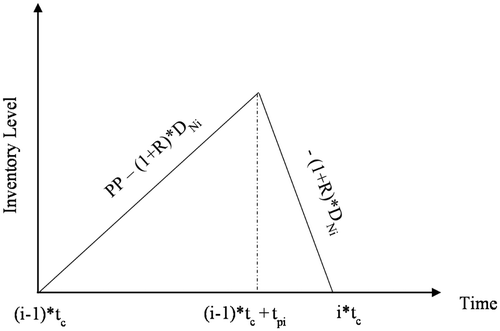
Considering the fact that some of the primary products are defective and will be returned by customers, the manufacturer has to produce more units and send more units to the market in order to satisfy the existing demand. Therefore, the primary products inventory level, I_ni(t), is given by:

where

tc	=	represents the duration of a cycle
DNi	=	represents the demand rate for primary products in the ith cycle
R	=	represents the return rate of primary products
PP	=	represents the production rate of primary products
tpi	=	represents the production period, i.e. manufacturing of primary products will continue until tpi and then there will be no products added to the primary products inventory because what has been produced will be sufficient to supply the demand

The boundary conditions for these differential equations are: I_ni(t) = 0 at and . The solution for these equations is expressed below:

Based on the values of the function in the boundaries we can find t_pi:

Figure 3 shows a schematic of the primary products inventory level at cycle i.

Figure 3. Primary products’ inventory level in the ith cycle.

As a result, the inventory cost for the primary products can be formulated as:

The production cost for manufacturing the primary products is assumed to be a decreasing function of the production rate define by parameters A₂, A₃ and A₄ as

A₂ is the set-up cost at the beginning of every cycle. Since the period under study and the length of a cycle are T and t_c, respectively, the total set-up cost, , is inversely proportional to the duration of a cycle. Assuming the sale price for a unit of primary product is ‘S_n’, the revenue from selling primary products during a cycle is:

3.2.2. Returned products inventory

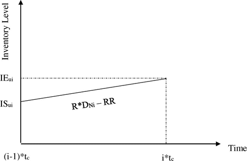
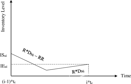
In order to formulate the returned products inventory, we need the associated boundary conditions. We assume that the returned products will be remanufactured at a constant rate of RR. At the beginning of the ith cycle, we have a number of returned products left in the inventory designated by IS_ui. Assuming that returned products in the ith cycle will be remanufactured in the next cycle (since transportation of the returned products from the retailers and sorting and making them ready for remanufacturing will take one cycle), the number of products available for remanufacturing in the ith cycle is equal to IS_ui.

The differential equation for the returned products inventory can be described as:

For the ease of formulation, we also use IE_ui as the level of returned products inventory in the end of the ith cycle. It can be seen that IE_ui = IS_u(i+1). With these initial conditions, we are able to solve the above differential equation:

We consider two different scenarios to calculate the initial condition for the i + 1th cycle and the inventory carrying costs of the ith cycle:

(A)

In this case, remanufacturing will continue until the end of the ith cycle at the given rate of RR. Therefore, at the end of the ith cycle we will be left with IEui returned products in the inventory: Therefore, the inventory costs can be calculated as: Figure 4 shows the inventory level for this case. It can be seen again that the remanufacturing process of the returned products will continue until the end of the ith cycle. Note that if then IEui > ISui and if then IEui < ISui.

(B)

In this case, it will take less than the duration of a cycle to remanufacture all the returned products. Therefore, remanufacturing process will continue until somewhere in the middle of the ith cycle at the given rate of RR and will stop until the end of the cycle. As a result, at the end of this cycle we will be left with only the products that have been returned during the ith cycle since everything else has been remanufactured: Therefore, the inventory costs can be calculated as: Figure 5 shows the inventory level for this case. It can be seen again that the remanufacturing process will continue until somewhere in the middle of the ith cycle at the given rate of RR and will stop at the end of the cycle.

Figure 4. Returned products’ inventory level in the ith cycle.

Figure 5. Returned products’ inventory level in the ith cycle.

3.2.3. Remanufactured products inventory

Similar to the returned products inventory, the associated boundary conditions with this inventory has to be calculated first. For the ease of formulation, we use IS_Ri and IE_Ri as the level of remanufactured products inventory in the beginning and end of the ith cycle, respectively.

Therefore, it can be seen that IS_R1 and IS_R2 are both equal to zero. In order to formulate the inventory level of remanufactured products we have to distinguish four different scenarios.

(A)	and In this case, the remanufacturing will continue until the end of the ith cycle at the given rate of RR. In addition, the second condition states that the demand for remanufactured product will be satisfied during this cycle. Therefore, the inventory level at the end of the ith cycle can be calculated as: Hence, the inventory costs can be calculated as: where A6 is the inventory carrying cost of a unit of remanufactured product per unit time. In this case, the total number of products being remanufactured is equal to . The remanufacturing cost calculation is presented in the next section. In addition, since all demands for remanufactured products will be satisfied with the selling price of Sr for remanufactured products, the profit made from selling these products would be equal to:
(B)	and Based on assumption 7 in Section 3.1, RR > DRi. Therefore, this scenario will never happen. It is intuitive that if the returned product inventory at the beginning of the ith cycle, ISui, is enough to remanufacture the products at a rate of RR, which is greater than DRi, the demand will certainly be satisfied.
(C)	and In this case, the remanufacturing process will continue until sometime in the middle of the ith cycle at the given rate of RR and will stop until the end of the cycle. In addition, the second condition states that the demand for remanufactured product will be satisfied during this cycle. Therefore, the inventory level at the end of the ith cycle can be calculated as: Hence, the inventory costs can be calculated as: In this case, the total number of products being remanufactured is equal to ISui. In addition, the demand for remanufactured products will be satisfied and the profit made from selling the remanufactured products would be equal to:
(D)	and In this case, the remanufacturing process will continue until sometime in the middle of the ith cycle at the given rate of RR and will stop until the end of the cycle. In addition, the second condition states that the demand for remanufactured product will not be satisfied during this cycle. Therefore, the inventory level at the end of the ith cycle will be equal to zero. Hence, the inventory costs can be calculated as: In this case, the total number of products being remanufactured is equal to ISui. In addition, the demand for remanufactured products will not be satisfied and on total ISRi + ISui remanufactured products will be sold at a price of Sr per unit. Therefore, the total profit made from selling the remanufactured products would be equal to:

3.2.4. Return rates and remanufacturing costs

An important factor in all of the above calculations is the return rate or R. In most available literature, this return rate is assumed to be a function of only the product quality, Ardeshirilajimi and Azadivar (2015b). Although this is certainly true, it is also true that different customers behave differently for a given product quality. In other words, given the quality of a particular unit of a product, one customer may decide to return the product while another customer may not. As a result, in this paper, the rate of return is affected by both the product quality and the customer tolerance for quality. In this paper we define customer tolerance by a customer preference function.

In this study, the product quality is defined in terms of the number of defective components it ends up to have when it reaches the customer. A product might consist of many parts, but a few parts might be the most important components for the operation or be the most susceptible to failure. We assume the number of these components to be n. Every part is manufactured with the targeted quality, p, which represents the probability of the part being defective.

To incorporate customer preference into return process in this study, we assume that the customers can be divided into J groups, namely group 0 to J − 1. For each group of customers we define S_j as the percentage of the entire customers population who fall in group j. Without loss of generality, the subscript j, 0 ≤ j ≤ J − 1, could be assigned such that customers in group j be those who would be satisfied with products with j or less defective parts. This characteristic will group customers according to their choosiness. For instance, group 0 refers to the choosiest customers who require products with zero defective parts. S₀, the percentage of customers who belong to this group can be any value between 0 and 100% based on the market and the type of product.

If we make the assumption that all parts have the same failure rate, the product received by a customer has k defective parts with a probability mass function of P(k):

The probability that this product will be accepted by a customer in group j is:

Therefore, the return percentage based on the customers’ groups can be calculated as:

With the return percentage formula calculated above, the cost of remanufacturing M returned products can be stated as:

where

Cremanuacturing	=	represents the total cost of remanufacturing a batch size of M units of returned products
Cdisassembly	=	represents the total cost of disassembly, inspection and sorting of a batch size of M units of returned products
Creassembly	=	represents the total reassembly cost of a batch size of M units of returned products
Cnew components	=	represents the total cost of buying new components to replace the defective ones in a batch size of M returned products

We assume that good components recovered from returned products are stored for each unit of remanufactured products and the defective components are replaced by new ones. We also assume that disassembly and reassembly costs for each remanufactured product are decreasing functions of the batch size. These decreasing functions can take many forms depending on the processes used for remanufacturing. Here, we approximate these costs with an exponential function of the batch size M as follows:

Now, we will calculate the total number of defective components that will be received based on the return rate calculated above. Let P(k) define the percentage of products with k or less defective components out of n.

The first group of customers, j = 0, will return products with even one defective component. In addition, products returned by group j, 0 ≤ j ≤ n, will result in receiving a returned product with k defective parts. Therefore, the total number of defective components to be replaced by new ones is equal to:

Here, for simplicity, we assume that the cost of all the components is equal, A₁₀. Therefore, assuming that in the ith cycle, M units of returned products will be remanufactured, the total cost of remanufacturing can be calculated as below:

where n is the total number of components in the final product.

3.2.5. Total profit function

Based on the above calculations, the total profit function in the time horizon T would be equal to:

Maximising this function is the objective of this paper. The decision variables are t_c, duration of a production cycle and p, the target production quality or defective rate of components.

4. Numerical examples

To illustrate the application of the presented method, several numerical examples with different assumptions have been studied. The numerical values assigned to parameters of the system are outlined below. It should be noted that these values are not based on a real case scenario. Any manufacturer interested in incorporating any part of the developed model to its supply chain management should pay careful consideration in attaining the exact values of these variables. A sensitivity analysis is performed at the following section of the paper to better demonstrate the effect of a change in the input variables, on the outputs of the model.

(1)	PP = 1500 units per day
(2)	RR = 150 units per day
(3)	Demand for primary products per day is a random variable that follows the normal distribution function of N(1000, 100)
(4)	Demand for remanufactured products per day is a random variable that follows the normal distribution function of N(100, 10)
(5)	0.0008 < p < 0.0012
(6)	T = 365 days
(7)	2 < tc < 10
(8)	A1 = 0.05
(9)	A2 = 150
(10)	A3 = 0.807
(11)	A4 = 991.9
(12)	A5 = 0.01
(13)	A6 = 0.03
(14)	A7 = 0.31
(15)	A8 = 0.001
(16)	A9 = 0.51
(17)	A10 = 0.001
(18)	A11 = 0.02
(19)	Sn = 1
(20)	Sr = 0.75

Table 3 summarises the results of optimum defective rate, optimum cycle length and maximum achievable profit with a 99% confidence intervals (CIs) for different customer satisfaction functions. For instance in the first case we consider that the 50% of the costumers require a product with zero defective components and 50% of the costumers do not mind receiving up to one defective component.

Table 3. Results of 99% CI for decision variables and objective function.

Case #	Satisfaction function	Variables	Mean	Standard deviation	99% CI
1		p^a	0.00200	1.7630 * 10^−5	[0.001996 0.002002]
		tc^b	5.88	0.33	[5.8 5.9]
		TP^c	292976	1559	[292743 293209]
2		p	0.003925	3.2004 * 10^−5	[0.003921 0.003930]
		tc	5.84	0.36	[5.8 5.9]
		TP	330061	1990	[329763 330359]
3		p	0.002562	2.2377 * 10^−5	[0.002560 0.002564]
		tc	5.87	0.34	[5.8 5.9]
		TP	311740	1672	[311550 311930]
4		p	0.005777	1.4279 * 10^−5	[0.005775 0.005778]
		tc	5.77	0.24	[5.7 5.8]
		TP	334257	2029	[334027 334488]

^a Defective rate.

^b Cycle length.

^c Total profit.

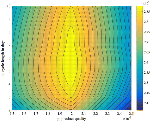
In order to emphasise the importance of choosing the optimum values for every variable, Figure 6 has been plotted for case number one. As it can be seen, from Figure 6, targeting a quality of parts used to manufacture primary products other than the optimal quality can result in significant loss of profit, in some cases even up to 50% of the net profit. In addition, the importance of choosing the optimum cycle length is clear. Choosing a short cycle will result in loss of profit due to unnecessary set-up costs and higher inventory costs.

Figure 6. Total profit function for case number one.

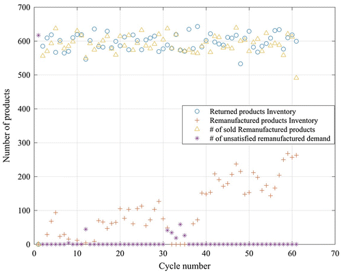
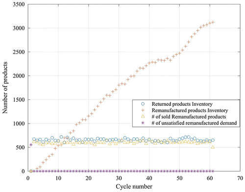
Moreover, Figure 7 shows the inventory levels for returned and remanufactured products for case number one when the optimum p value is chosen. It can be seen that in almost all the cycles the demand for remanufactured products is satisfied. In addition, the inventory levels of remanufactured and returned products are always relatively low, which prevents high inventory costs.

Figure 7. Inventory level for a for p = 0.00200 and t_c = 6.

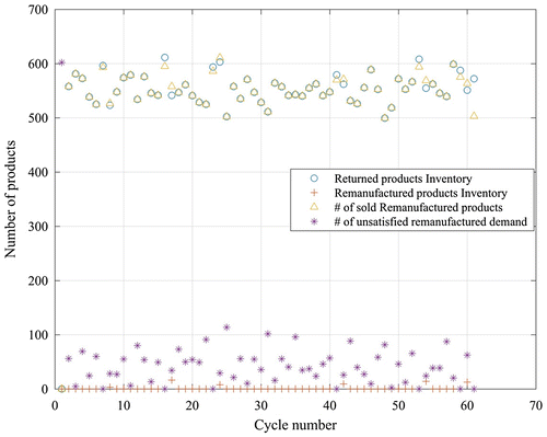
Figure 8 shows the same case when a lower than optimal quality (defective rate) is chosen. A lower defective rate will result in fewer returned products. As it can be seen in Figure 8, almost all the returned products are remanufactured in every cycle. However, it can be seen that in almost all the cycles the demand for remanufactured products is not satisfied. This is a direct result of not having enough returned products to remanufacture. Moreover, the inventory level of remanufactured products is zero at almost every cycle since all the products in that inventory is sold to satisfy the demand.

Figure 8. Inventory level for a for p = 0.00184 and t_c = 6

Figure 9 shows the same case when a higher than optimal defective rate is chosen. A higher defective rate will result in more returned products. Although the demand for remanufactured products is always getting satisfied, the inventory level for remanufactured products are considerably large, which will result in a significant loss in profit.

Figure 9. Inventory level for a for p = 0.00220 and t_c = 6.

4.1. Sensitivity analysis

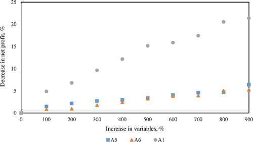
In order to measure sensitivity of this analysis with respect to numerical values assigned to systems parameters, a sensitivity analysis was performed with respect to inventory carrying costs. Figure 10 presents the result of this analysis on A₁, A₅ and A₆ which represent inventory carrying costs for a unit of primary product, returned product and remanufactured product, respectively. The sensitivity analysis was performed by increasing the value of these parameters and calculating the optimum total profit. It can be seen that the model is more sensitive to a change in A₁ as compared to A₅ and A₆. This can be the result of higher number of primary products compared to returned and remanufactured products.

Figure 10. Sensitivity analysis for different inventory carrying costs.

5. Conclusion

In this article, we investigate the profit maximisation for a manufacturing/remanufacturing unit that uses three inventories, one for primary, one for returned and one for remanufactured products. In addition, we consider two independent demands for primary and remanufactured products. These demands are assumed to be random variables.

Customers return items at a rate that depends on two factors: The targeted quality of parts that were used to manufacture the primary products, and the customer satisfaction function. At the end of every cycle, good parts recovered from returned products are used to remanufacture aftermarket products to satisfy the demand for remanufactured products. It is possible that the accumulated returned products provide components that are more than what is needed to satisfy the demand for remanufactured products. In this case, the remaining remanufactured products are stored in the remanufactured products inventory to be used in the next cycle. On the other hand, the returned products inventory might not be enough to satisfy this demand. In which case, the manufacturer simply cannot profit from such demand. No costs with respect to the inability of manufacturer to satisfy the aftermarket demand were considered in the model.

It is shown that inventory levels and the total profit for the system could be significantly influenced by the duration of accumulation of returned products before remanufacturing and the targeted product quality. A model is developed to obtain the optimum values for the production cycle time for manufacturing and remanufacturing products and the target quality for parts used to manufacture primary products. Using the model, a formulation is derived for optimisation of these parameters to maximise the total expected profit for the system. Several numerical examples have shown that the expected profit will decrease substantially, in some cases up to 50%, if one does not choose the optimal values for these decision variables.

The model can be extended by assuming different levels of quality (defective rate of parts) for each one of the parts in a product. This is a realistic assumption since not all parts are equally susceptible to fail. Moreover, if the volume of returns is significantly large, the model can be extended to account for the remanufactured products that are returned by consumers as well. Although since this number will be of second order of significance, this addition may not make considerable difference for moderate production volumes. Consequently, one could look for production volumes that would justify this extension.

Notes on contributors

Ardavan Ardeshirilajimi is a PhD student in the Department of Civil and Environmental Engineering at University of Illinois at Urbana-Champaign. He received his master’s degree in Mechanical Engineering from University of Massachusetts Dartmouth. His research interest includes reverse supply chain, inventory systems, and remanufacturing of commercial returns.

Farhad Azadivar is a professor in the Department of Mechanical Engineering at University of Massachusetts Dartmouth. Prior to that he has served as the dean of College of Engineering at UMASS Dartmouth and the director of Advanced Manufacturing Institute at Kansas State University. His research interests include discrete systems simulation, simulation optimisation and the application of simulation based optimisation to manufacturing, robotics, transportation, and fishery systems.

Disclosure statement

No potential conflict of interest was reported by the authors.

References

- Alinovi, Alberto, Eleonora Bottani, and Roberto Montanari. 2012. “Reverse Logistics: A Stochastic EOQ-based Inventory Control Model for Mixed Manufacturing/Remanufacturing Systems with Return Policies.” International Journal of Production Research 50 (5): 1243–1264.10.1080/00207543.2011.571921
- Ardeshirilajimi, Ardavan, and Farhad Azadivar. 2015a. “Remanufacturing of Commercial Returns in a Market with a Variable Quality Tolerance.” In 2015 International Conference on Industrial Engineering and Operations Management (IEOM), Dubai, 1–6.10.1109/IEOM.2015.7093946
- Ardeshirilajimi, Ardavan, and Farhad Azadivar. 2015b. “Reverse Supply Chain Plan for Remanufacturing Commercial Returns.” The International Journal of Advanced Manufacturing Technology 77 (9–12): 1767–1779.10.1007/s00170-014-6509-9
- Blackburn, Joseph D., V. Daniel R. Guide, Gilvan C. Souza, and Luk N. Van Wassenhove. 2004. “Reverse Supply Chains for Commercial Returns.” California Management Review 46 (2): 6–22.10.2307/41166207
- Davey, Sylvia, V. Daniel R. Guide Jr., Kumar Neeraj, and Luk N. Van Wassenhove. 2005. “Commercial Returns of Printers: The HP Case.” In Managing Closed-loop Supply Chains, 87–96. Berlin: Springer.
- Dobos, Imre. 2003. “Optimal Production–Inventory Strategies for a HMMS-type Reverse Logistics System.” International Journal of Production Economics 81–82: 351–360.10.1016/S0925-5273(02)00277-3
- Dobos, Imre, and Knut Richter. 2004. “An Extended Production/Recycling Model with Stationary Demand and Return Rates.” International Journal of Production Economics 90 (3): 311–323.10.1016/j.ijpe.2003.09.007
- Feng, Lin, Jianxiong Zhang, and Wansheng Tang. 2013. “Optimal Control of Production and Remanufacturing for a Recovery System with Perishable Items.” International Journal of Production Research 51 (13): 3977–3994.
- Fleischmann, Moritz, and Stefan Minner. 2004. “Inventory Management in Closed Loop Supply Chains.” In Supply Chain Management and Reverse Logistics, 115–138. Berlin: Springer.
- Fleischmann, Moritz, Jo A. E. E. van Nunen, and Ben Gräve. 2003. “Integrating Closed-loop Supply Chains and Spare-parts Management at IBM.” Interfaces 33 (6): 44–56.10.1287/inte.33.6.44.25189
- Gallagher, Tim, Mark D. Mitchke, and Matthew C. Rogers. 2005. “Profiting from Spare Parts.” The McKinsey Quarterly 2: 1–4.
- Gu, Qiaolun, and George Tagaras. 2014. “Optimal Collection and Remanufacturing Decisions in Reverse Supply Chains with Collector’s Imperfect Sorting.” International Journal of Production Research 52 (17): 5155–5170.
- Guide Jr., V. Daniel R., Gilvan C. Souza, Luk N. Van Wassenhove, and Joseph D. Blackburn. 2006. “Time Value of Commercial Product Returns.” Management Science 52 (8): 1200–1214.10.1287/mnsc.1060.0522
- Hsueh, Che-Fu. 2011. “An Inventory Control Model with Consideration of Remanufacturing and Product Life Cycle.” International Journal of Production Economics 133 (2): 645–652.10.1016/j.ijpe.2011.05.007
- Hsueh, Che-Fu. 2015. “A Decentralized Production/Remanufacturing Inventory Model with Multiple Refurbished Components.” Engineering Management Research 4 (2): 34.
- Kiesmüller, Gudrun P., and Erwin A. van der Laan. 2001. “An Inventory Model with Dependent Product Demands and Returns.” International Journal of Production Economics 72 (1): 73–87.10.1016/S0925-5273(00)00080-3
- van der Laan, Erwin, Marc Salomon, and Rommert Dekker. 1999. “An Investigation of Lead-time Effects in Manufacturing/Remanufacturing Systems under Simple PUSH and PULL Control Strategies.” European Journal of Operational Research 115 (1): 195–214.10.1016/S0377-2217(98)00108-8
- Poles, Roberto. 2013. “System Dynamics Modelling of a Production and Inventory System for Remanufacturing to Evaluate System Improvement Strategies.” International Journal of Production Economics 144 (1): 189–199.10.1016/j.ijpe.2013.02.003
- Richter, Knut, and Mirko Sombrutzki. 2000. “Remanufacturing Planning for the Reverse Wagner/Whitin Models.” European Journal of Operational Research 121 (2): 304–315.10.1016/S0377-2217(99)00219-2
- Shen, Zuo-Jun Max, Collette Coullard, and Mark S. Daskin. 2003. “A Joint Location-inventory Model.” Transportation Science 37 (1): 40–55.10.1287/trsc.37.1.40.12823
- Vercraene, Samuel, Jean-Philippe Gayon, and Simme Douwe Flapper. 2014. “Coordination of Manufacturing, Remanufacturing and Returns Acceptance in Hybrid Manufacturing/Remanufacturing Systems.” International Journal of Production Economics 148: 62–70.10.1016/j.ijpe.2013.11.001