Production disruption management for R/M integrated supply chain using system dynamics methodology

Abstract

The impacts of production disruption in Remanufacturing/Manufacturing (R/M) integrated supply chain on the sales and the methods of production disruption management were studied. A system dynamics model for the R/M integrated supply chain with production disruption was improved by system dynamics methodology. The numerical examples were shown to illustrate the simulation results. The impacts of different recovery times of production disruption on the sales were presented. In order to mitigate the disruption risks and ensure the sales at the needed sales ratio, the methods for setting multi-echelon inventory levels before the occurring of the production disruption and the methods for making back-up plans after the production disruption occurs were given.

Keywords:

• Production disruption
• R/M integrated supply chain
• system dynamics
• risk mitigation

1. Introduction

Production disruption is one kind of supply chain disruptions that may result in severe consequences. For example, the Taiwan earthquake in 1999 is a typical example that reflects the tremendous impact of supply disruptions. Taiwan was the third largest supplier of computer accessories in the world at that time. The earthquake caused a two-week global semiconductor shortage, and thereby undermined countless companies all over the world (Li and Chen 2010). It was the two-week global semiconductor shortage that caused the relevant companies had to face their production disruptions.

No matter what the reason of the production disruption is, how to react or manage the disruption is very important for all the members of the supply chain. For instance, the lightning incident in 2000 catastrophically destroyed a Phillips Electronics semiconductor plant, which was Ericsson’s sole supplier. As a result, Ericsson reported a $400 million loss because it did not receive chip deliveries from the Philips plant in a timely manner. However, Nokia, a competitor of Ericsson, immediately sensed the disruption and responded aggressively. Nokia’s share of the handset market increased from 27 to 30% because Nokia has taken better measures (Latour 2001).

In general, the strategies of mitigating the disruption of supply chain include: increase the inventory level and back up from other suppliers. But, the inventory level and the back-up plans should be adjusted when the disruption lasts for different periods. The aims of this paper are to find new methods for setting multi-echelon inventory levels before the occurring of the production disruption and to find new methods for making back-up plans after the production disruption occurs in Remanufacturing/Manufacturing (R/M) integrated supply chain.

The R/M integrated supply chain is a closed-loop supply chain which includes the forward supply chain and the reverse supply chain. The manufacturer is the core member who will carry out remanufacturing and manufacturing simultaneously. Note that, if the remanufacturing is carried out by another assigned remanufacturer, the supply chain is an open form of ‘R/M’ which is not under consideration in this study.

In the R/M integrated supply chain, the manufacturer makes new products by assembling new parts or remanufactured parts. The new products are made and sold to the end-customer via the forward supply chain. After using, these new products become used products. In reverse supply chain, the collector is responsible for collecting the used product from the end customers. The disassembly centre purchases the used products from the collector, and then, the disassembly centre offers the reusable product to the consumer market after simple treating. For the non-reusable products, after disassembling, the disassembly centre offers the remanufacturable parts and the recyclable materials to the manufacturer and the parts producer, respectively. Of course, some trash may also be produced in this process.

In this study, the production disruption of the manufacturer is considered, and the main questions are focused on:

•	What are the impacts of different recovery time of production disruption on the sales?
•	How to set the multi-echelon inventory levels to ensure the sales at the needed sales ratio before the disruption occurs?
•	How to make the back-up plans to ensure the sales at the needed sales ratio after the occurring of the disruption?

Motivated by these questions, a system dynamics model for the R/M integrated supply chain with production disruption is given using the Vensim 5.10. By the numerical example and simulation results, the impacts of different recovery times of production disruption on the sales are illustrated, and the methods for setting multi-echelon inventory levels and for making back-up plans are presented.

The paper is organised by following sections: in Section 2, the relative literatures are reviewed. In Section 3, the system dynamics model with the production disruption is proposed. In Section 4, the impacts of different recovery times of production disruption on the sales are illustrated, and the methods for setting multi-echelon inventory levels and making back-up plans to ensure the sales at the needed sales ratio are given. In Section 5, the sensitivity analyses are presented. The results of this study and the further research directions are summarised in Section 6.

2. Literature review

The relevant literature to this study includes four parts: disruption management of supply chain, disruption management of supply chain by system dynamics methodology, application of system dynamics methodology in supply chain with remanufacturing and disruption management of supply chain with remanufacturing by system dynamics methodology.

There are many research results for the disruption management of supply chain. Rice and Caniato (2003) surveyed a company and estimated that the daily cost impact of a disruption in its supply network to be in $50–$100 million or so. Qi, Bard, and Yu (2004) investigated a one-supplier-one-retailer supply chain that experiences a disruption in demand during the planning horizon, and they showed that changes to the original plan induced by a disruption may impose considerable deviation costs throughout the system. Xia, Xiao, and Yu (2004) studied a lot-for-lot production and inventory system with the raw material supply disruptions that result in the fluctuation of the production cost. Yang, Qi, and Yu (2005) proposed a dynamic programming method for the demand and cost disruption management of a firm. Xiao and Yu (2006) developed an indirect evolutionary game model with two-vertically integrated channels to study evolutionarily stable strategies of retailers in the quantity-setting duopoly situation with homogeneous goods and analysed the effects of the demand and raw material supply disruptions on the retailers’ strategies. Xiao and Qi (2008) studied the coordination of a supply chain with one manufacturer and two competing retailers after the production cost of the manufacturer was disrupted. They also extended the model to the case with both cost and demand disruptions. Chen and Xiao (2009) developed two coordination models of a supply chain with one manufacturer, one dominant retailer and multiple fringe retailers to investigate how to coordinate the supply chain after demand disruption. They also found that the disrupted amount of demand largely affects the allocation of the supply chain’s profit. Yu, Zeng, and Zhao (2009) gave a risk evaluation for the impacts of supply disruption on the choice between the famous single and dual sourcing methods in a two-stage supply chain with a non-stationary and price-sensitive demand. They obtained the expected profit functions for the two sourcing modes in the presence of supply chain disruption risks, and examined the sensitivity of the buyer’s expected profit to various input factors through numerical examples. Cauvin, Ferrarini, and Tranvouez (2009) proposed an approach to minimise the impact of disrupting events on the whole system. It is based on an analysis of disrupting events and the characterisation of the recovery process, and on a cooperative repair method for distributed industrial systems.

Management of disruption of supply chain by system dynamics has also received attention. Wilson (2007) investigated the effect of a transportation disruption on supply chain performance using system dynamics simulation, he gave some comparison between a traditional supply chain and a vendor managed inventory (VMI) system when a transportation disruption occurs between two echelons in a five-echelon supply chain. Jain (2010) investigated the impact of supply disruption between any two players on the performance of a multiplayer supply chain system with Retailer, Wholesaler, Distributor and Factory. Chen, Li, and Shi (2011) employed system dynamics to construct a traditional supply chain model, a pipeline-inventory-control supply chain model and a VMI supply chain model in order to study the long-run effect of disruptions on supply chain performance. Lorentz and Hilmola (2012) introduced a continuous simulation model that is based on a Bayesian robot decision-maker, and illustrated the process of evaluating competing hypotheses of functional vs. dysfunctional supply chain design in a disruption scenario by the system dynamics approach.

As for the application of system dynamics methodology in supply chain with remanufacturing, Vlachos, Georgiadis, and Iakovou (2007) tackled the development of efficient capacity planning policies for remanufacturing facilities in reverse supply chains, taking into account not only economic but also environmental issues, such as the take-back obligation imposed by legislation and the ‘green image’ effect on customer demand. In their study, there are only two echelons (producer and distributor) in the forward supply chain, and there is only one reuse activity (remanufacturing) in the reverse channel. Georgiadis and Besiou (2008) examined the impact of ecological motivation and technological innovations on the long-term behaviour of a closed-loop supply chain with recycling activities using system dynamics methodology. There are two echelons (producer and distributor) in the forward supply chain, and one reuse activity is recycling in the reverse channel. Gu and Gao (2012a) proposed a system dynamics model to examine the long-term behaviour of the R/M integrated supply chain with reuse, remanufacturing, and recycling. Based on the simulation results, they gave the joint decisions for R/M integrated supply chain. By system dynamics methodology, Papachristos (2014) presented a capital goods supply chain model where retailers initiated remanufacturing operations and competed against OEM brand products. Wang et al. (2014) explored the impact of subsidy policies on the development of the recycling and remanufacturing industry in China using system dynamics methodology.

Regarding the disruption management of supply chain with remanufacturing by system dynamics methodology, Gu and Gao (2012b) presented a system dynamics model with supply disruption of key remanufactured parts to estimate the remanufacturer’s profit, and chose a strategy to ensure that the remanufacturer does not incur a loss when the supply disruption lasts for a long time. Gu, Tagaras, and Gao (2014) examined reverse supply chains consisting of three members (collector, disassembly centre and remanufacturer) and subjected to four different types of supply disruption, each with distinct impact on the members of the chain. Using system dynamics methodology, they focused on the quantitative method of disruption risk evaluation by simulation analysis of the impacts of each supply disruption on the Mean profits of the various supply chain member.

In this paper, the disruption management of supply chain will be studied by using system dynamics methodology. The differences between this study and the above papers are as follows. Firstly, they considered the transportation disruption or supply disruption, while this paper discusses the production disruption owing to supply disruption or natural disasters. Secondly, they focused on comparing the impacts of the disruptions occurred in different echelon or giving the method to mitigate the impacts when the disruption occurred, while this paper focuses on the impacts of production disruption on the consumer market from the manufacturer’s point of view and presents the methods of setting multi-echelon inventory levels before the disruption occurs and make back-up plans after the production disruption occurs.

The previous study that is most closely related to the present paper is the results of Gu and Gao (2012a). They developed a system dynamics model of the R/M integrated supply chain by Vensim 5.10 and gave the joint decisions for R/M integrated supply chain. However, they didn’t consider any disruptions of the supply chain. Based on the model of the R/M integrated supply chain in their study, the present study will show the model with production disruption of the R/M integrated supply chain by adding disruption elements, and present the study results.

3. Model description

3.1. Model structure

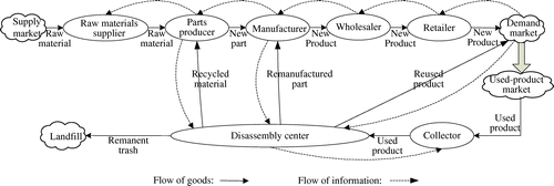
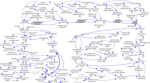
The structure of the R/M integrated supply chain under study is shown in Figure 1. The R/M integrated supply chain has seven members: the raw materials supplier, the parts producer, the manufacturer, the wholesaler, the retailer, the collector and the disassembly centre. Figure 1 shows the relationship of goods flow and information flow between these members. The detailed description of the model structure is shown in the causal loop diagram developed by using Vensim 5.10 (Figure 2). All explanations of the variables and constants involved in Figure 2 can be found in reference Gu and Gao (2012a).

Figure 1. Flow of goods and information in R/M integrated supply chain.

Figure 2. Causal loop diagram of R/M integrated supply chain.

The raw materials’ supplier obtains the raw materials from the supply market, and transports them to the parts producer according to the order of raw materials.

The parts producer produces the new parts using two flows of materials: raw materials and recycled material. Of course, after recycling by the disassembly centre (or other recycling plant), the recycled material must become the material as good as the material that comes from the raw materials’ supplier. The parts producer receives the recycled materials from the disassembly centre, sends the order information of raw materials to the raw materials supplier, and transports the new parts to the manufacturer based on the order of the new parts.

The manufacturer makes the new products using two flows of parts: new parts from the parts supplier and remanufactured parts from the disassembly centre. Of course, after remanufacturing by the disassembly centre (or other remanufacturing plant), the remanufactured parts must become the parts as good as the new parts. The manufacturer receives the remanufactured parts from the disassembly centre, sends the order information of new parts to the parts producer, and transports the new products to the wholesaler based on the order of the new products.

The wholesaler purchases the products from the manufacturer, sends the order information of new products to the manufacturer, and transports the new products to the retailer according to the order of the new products.

The retailer purchases the products from the wholesaler, sends the order information of new products to the wholesaler, and sells the new products to the market considering the market demand of the new products.

The collector collects the used-products from the used-product market considering the need of the used-products. These collected used-products are sold to the disassembly centre.

The disassembly centre purchases the used products from the collector, tests and disassembles these used products so as to get the reusable product, the remanufacturable parts, the recyclable materials and the trash. The disassembly centre offers the reused products to the market considering the information comes from the market, offers the remanufactured parts to the manufacturer according to the need information comes from the manufacturer, and offers the recycled materials to the parts producer considering the need information comes from the parts producer.

This paper focuses on the sales marked by a circle as well as Manufacturer’s Inventory, Wholesaler’s Inventory and Retailer’s Inventory marked by grey colour in Figure 2. The goal is to study the impacts of production disruption in R/M integrated supply chain on the sales and the methods of production disruption management to ensure the sales at the needed sales ratio.

3.2. Stock-flow diagram with production disruption

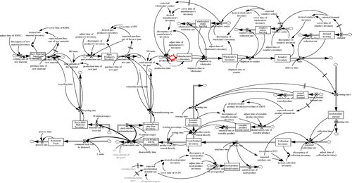
The stock-flow diagram with production disruption of the R/M integrated supply chain is shown in Figure 3. Just like the above description, this stock-flow diagram is improved from reference Gu and Gao (2012a) by adding some changes. Therefore, only the changes are given here to avoid the same contents of the variables, constants and equations as that in Gu and Gao (2012a). The differences are listed in Table 1.

Figure 3. Stock-flow diagram of R/M integrated supply chain with production disruption.

Table 1. Differences between the stock-flow diagram with and without production disruption.

In stock-flow diagram with production disruption	In stock-flow diagram without production disruption (Gu and Gao, 2012a)
Production rate = IF THEN ELSE (Time ≥ i: AND: Time ≤ j, 0, expected wholesaler’s orders + discrepancy of manufacturer’s inventory/adjust time of manufacturer’s inventory)	Production rate = expected wholesaler’s orders + discrepancy of manufacturer’s inventory/adjust time of manufacturer’s inventory
Demand = RANDOM NORMAL (Minimum Value, Maximum Value, Mean, Standard Deviation, Initial Value)	Demand = potential demand market/demand time
<Time>	–
–	Potential demand market
–	Demand time
Manufacturer’s Inventory = INTEG (IF THEN ELSE (Time = k1, Mean of Manufacturer’s Inventory × α1, production rate − shipment to wholesaler))	Manufacturer’s Inventory = INTEG (production rate − shipment to wholesaler, 0)
Wholesaler’s Inventory = INTEG (IF THEN ELSE (Time= k2, Mean of Wholesaler’s Inventory × α2, shipment to wholesaler − shipment to retailer))	Wholesaler’s Inventory = INTEG (shipment to wholesaler − shipment to retailer, 0)
Retailer’s Inventory = INTEG(IF THEN ELSE (Time = k3, Mean of Retailer’s Inventory × α3, shipment to retailer − sales))	Retailer’s Inventory = INTEG (shipment to retailer − sales, 0)

The equation of production rate in stock-flow diagram with production disruption means that: if a production disruption happens at the ith period and lasts to the jth period, the values of production rate in these periods are 0; otherwise, the values of production rate are ‘expected wholesaler’s orders + discrepancy of manufacturer’s inventory/adjust time of manufacturer’s inventory’. Herein, i and j are simulation periods, and i ≤ j, namely, the production disruption lasts for j − i periods.

In the equation of demand in stock-flow diagram with production disruption, RANDOM NORMAL () is a Normal Distribution function with five parameters: Minimum Value, Maximum Value, Mean, Standard Deviation and Initial Value.

<Time> is a shadow variable in stock-flow diagram with production disruption, it is used to describe the occurring and the ending of the production disruption.

Potential demand market and demand time which are used in stock-flow diagram without production disruption are deleted from the present stock-flow diagram.

In the equations of Manufacturer’s Inventory, Wholesaler’s Inventory and Retailer’s Inventory, INTEG () is the function that defines a level variable (integrating the variable over time). Mean of Manufacturer’s Inventory, Mean of Wholesaler’s Inventory and Mean of Retailer’s Inventory are the average values of Manufacturer’s Inventory, Wholesaler’s Inventory and Retailer’s Inventory with no production disruption, respectively. k1, k2 and k3 are the periods during which the inventory quantities will be added and the adding rates are α1, α2 and α3, respectively.

All of the other variables and equations used in the Stock-flow diagram with production disruption can be found in Gu and Gao (2012a). In order to facilitate the description of present paper, these variables and equations are list in Appendix A.

4. Numerical illustration

In this section, the numerical illustrations are based on the following assumptions: The R/M integrated supply chain described above has been successfully carried out via adopting the joint decisions given by Gu and Gao (2012a); The manufacturer confronts a potential risk of production disruption. As the core member of the R/M integrated supply chain, the manufacturer plans to find some efficient methods for mitigating the potential risk of production disruption. Therefore, these methods will be explored by next numerical example.

The exploration continues the study in Gu and Gao (2012a). There is a key parameter r in Gu and Gao (2012a), and r = STEP (u, v). Here, u stands for the remanufacturing ratio, and v stands for the setup period of remanufacturing. STEP (b, m) means that the manufacturer will carry out remanufacturing from the vth period and the remanufacturing ratio is u. According to the research results of Gu and Gao (2012a), the remanufacturer can choose the optimal values of r: r = STEP (0.1, 7), r = STEP (0.2, 8), r = STEP (0.3, 8), r = STEP (0.4, 8), r = STEP (0.5, 8), r = STEP (0.6, 9), r = STEP (0.7, 9), r = STEP (0.8, 10), r = STEP (0.9, 10) and r = STEP (1, 11). In the next simulation, r = STEP (0.5, 8), r = STEP (0.3, 8) and r = STEP (0.7, 9) will be chosen as the value of r.

Without loss of generality, in this numerical example, it’s assumed that the manufacturer has started the remanufacturing at 8th week and the remanufacturing ratio is 0.5, namely, r = STEP (0.5, 8). A production disruption occurs at the 21st week. The manufacturer can recover the production during T-week (T = 1, 2, 3, 4, 5, 6). Namely, the production recovery time is T-week. The demand is ‘RANDOM NORMAL (8000, 12000, 10000, 2000, 10000)’. Other parameters values are listed in Table 2.

Table 2. Parameter settings.

Parameter	Member
	Manufacturer	Wholesaler	Retailer	Parts producer	Raw materials supplier	Collector	Disassembly centre
Initial value of inventory	0	0	0	1000	100000	0	0
Adjust time of inventory	3	3	3	3	3	3	3
Cover time of inventory	1; 1.5; 2; 2.5; 3	1; 1.5; 2; 2.5; 3	1; 1.5; 2; 2.5; 3	2	1.5	2	1.5
Lead time	2	1	1.5	1.5		2	2
Production time	2			1.5			1.5

Based on the model described in Section 3 and by this example, the impacts of different recovery time of production disruption on the sales are presented in Subsection 4.1. In order to mitigate the disruption risks and ensure the sales ratio, methods for setting multi-echelon inventory levels before the occurring of the production disruption and methods for making back-up plans after the production disruption occurs are given in Subsections 4.2 and 4.3.

4.1. Impacts of different recovery time of production disruption on the sales

When the production disruption occurs at the 21st week and the recovery time is T-week (T = 1, 2, 3, 4, 5 and 6), the production rate under each recovery time can be expressed, respectively:(1)

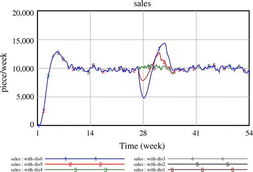
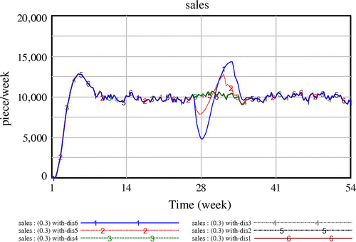
Where cover time of manufacturer’s inventor, cover time of wholesaler’s inventory and cover time of retailer’s inventory are 1.5 weeks, 1 week and 1.5 weeks, respectively. The simulation results of the impacts of different recovery time of production disruption on the sales are shown in Figure 4(a). In Figure 4(a), with-disT is the simulation result when the recovery time is T-week (T = 1, 2, 3, 4, 5 and 6).

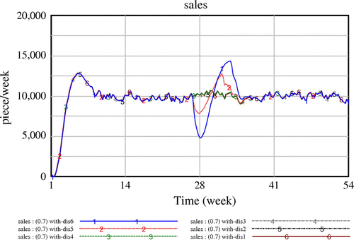
Figure 4. (a) Impacts of different recovery time of production disruption on the sales (r = STEP (0.5, 8)), (b) Impacts of different recovery time of production disruption on the sales (r = STEP (0.3, 8)), (c) Impacts of different recovery time of production disruption on the sales (r = STEP (0.7, 9)).

Figure 4(a) shows that all the sales are not affected if the recovery time is one-week (two-week, three-week and four-week) or if the production disruption can be recovered during four weeks from the disruption’s starting. However, if the recovery time is longer than four weeks, the sales will be affected by the production disruption: the longer the production disruption recovery time is, the larger the sales fluctuation is.

Obviously, the sales fluctuation is the production disruption risk for the members of R/M integrated supply chain. How to mitigate the sales fluctuation is the main aim of this study.

In order to mitigate the sales fluctuation, Subsections 4.2 and 4.3 focus on how to set the multi-echelon inventory levels and how to make the back-up plans when the recovery time is 6-week.

Before investigating the mitigation methods, other two questions need to be discussed. In this numerical example, the remanufacturing starts from the 8th period and the remanufacturing ratio is 0.5, namely, r = STEP (0.5, 8). How about the sales fluctuation if the remanufacturing ratio is not 0.5 and the remanufacturing starts from other different period? Further simulating results (Figure 4(b) and 4(c)) show that the sales fluctuations under different remanufacturing ratios or different starting period have the same behaviours as Figure 4(a). Such as, in Figure 4(b), the remanufacturing start from the 8th period and the remanufacturing ratio is 0.3, namely, r = STEP (0.3, 8); in Figure 4(c), the remanufacturing starts from the 9th period and the remanufacturing ratio is 0.7, namely, r = STEP (0.7, 9). Note that, r = STEP (0.3, 8) and r = STEP (0.7, 9) are chosen from the optimal values of r. This indicates that the choice of r = STEP (0.5, 8) in this numerical example is reasonable and effective.

4.2. Method for setting multi-echelon inventory levels

Before the occurring of the production disruption, the impacts of the production disruption on the sales can be eliminated by setting multi-echelon inventory levels. In this model, the multi-echelon inventory levels will be set via choosing the cover time of manufacturer’s inventor, cover time of retailer’s inventory and cover time of wholesaler’s inventory following the three steps. After the three steps, the sales fluctuation disappears.

4.2.1. Step-1: choosing cover time of manufacturer’s inventory

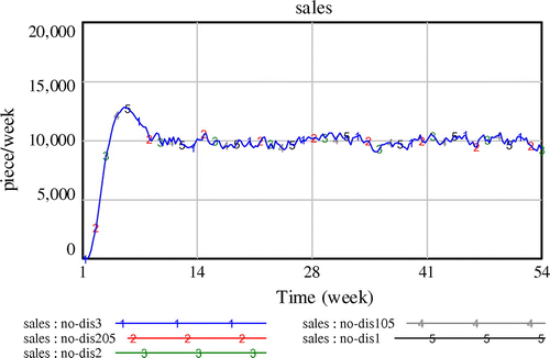
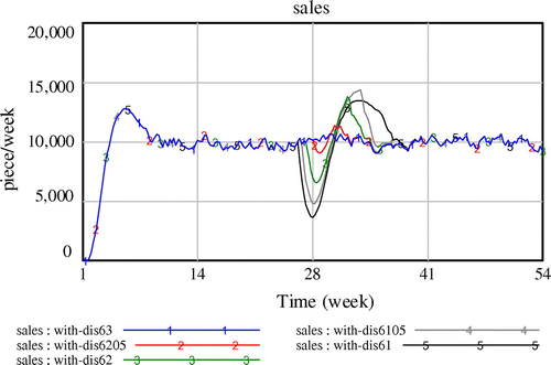
In simulation, cover time of wholesaler’s inventory = 1, cover time of retailer’s inventory = 1.5. The simulation results without production disruption (no-disT1) and with production disruption (with-dis6T1) are shown in Figure 5 and Figure 6, respectively. Herein, T1 = 1, 105, 2, 205 and 3 correspond to the cover time of manufacturer’s inventory = 1, 1.5, 2, 2.5 and 3 respectively.

Figure 5. Sales with different cover time of manufacturer’s inventory (no disruption).

Figure 6. Sales with different cover time of manufacturer’s inventory (with 6 weeks disruption).

Figure 5 shows that the sales behaviours are the same even though the cover time of manufacturer’s inventory takes different values. Namely, if there is no production disruption, the sales is normal no matter what the value of cover time of manufacturer’s inventory is. If there is a six weeks production disruption (Figure 6), the sales fluctuations appear from some periods. Table 3 shows the comparisons between the sales no disruption and the sales with six weeks disruption.

Table 3. Sales comparisons of no disruption and with 6 weeks disruption.

Cover time of manufacturer’s inventory		Sales at each period
		26th	27th	28th	29th	30th	31th	32th	33th	34th
3 weeks	With 6 weeks disruption	10,265	10,253	10,250	10,230	10,254	10,202	9,608	10,422	9,996
	No disruption	10,265	10,253	10,250	10,230	10,254	10,202	9,608	10,422	9,996
	Sales ratio	1.00	1.00	1.00	1.00	1.00	1.00	1.00	1.00	1.00
2.5 weeks	With 6 weeks disruption	10,265	10,253	9,179	9,655	11,386	10,692	9,763	10,471	10,012
	No disruption	10,265	10,253	10,250	10,230	10,254	10,202	9,608	10,422	9,996
	Sales ratio	1.00	1.00	0.90	0.94	1.11	1.05	1.02	1.00	1.00
2 weeks	With 6 weeks disruption	10,265	8,737	6,567	8,237	10,740	12,918	12,321	11,280	10,268
	No disruption	10,265	10,253	10,250	10,230	10,254	10,202	9,608	10,422	9,996
	Sales ratio	1.00	0.85	0.64	0.81	1.05	1.27	1.28	1.08	1.03
1.5 weeks	With 6 weeks disruption	10,265	5,704	5,053	7,412	10,401	12,680	13,910	14,344	11,553
	No disruption	10,265	10,253	10,250	10,230	10,254	10,202	9,608	10,422	9,996
	Sales ratio	1.00	0.56	0.49	0.72	1.01	1.24	1.45	1.38	1.16
1 week	With 6 weeks disruption	8,203	4,025	4,139	6,860	10,020	12,243	13,260	13,477	13,144
	No disruption	10,265	10,253	10,250	10,230	10,254	10,202	9,608	10,422	9,996
	Sales ratio	0.80	0.39	0.40	0.67	0.98	1.20	1.38	1.29	1.31

Note: The bold value means the lowest sales ratio from 26th period to 34th period.

In Table 3, sales ratio stands for the changes of sales owing to the production disruption:

(2)

For example, when cover time of manufacturer’s inventory is 2.5 weeks, sales ratio is equal to 0.90 at 28th period. This means the sales with disruption is only 90 per cent of the sales no disruption.

Table 4 (Step-1) shows the lowest sales ratio under different combination of inventory level with six weeks disruption of Step-1. From Table 4, when cover time of wholesaler’s inventor is 1 and cover time of retailer’s inventory is 1.5, the manufacturer should set the cover time of manufacturer’s inventory is no shorter than 2.5 weeks (3 weeks, 2 weeks, 1.5 weeks and 1 week) so as to ensure that the sales ratio at every period is no less than 90% (100, 64, 49 and 39%). Herein, the shortest one which satisfies the relevant condition is chosen. Note that, this is the choice rule used in this paper.

Table 4. Lowest sales ratio under different combination of inventory level with 6 weeks disruption.

Steps	Combination of each member’s inventory cover time (week)			Lowest sales ratio (occurred period)
	Manufacturer	Wholesaler	Retailer
Step-1	3	1	1.5	100% (all)
	2.5	1	1.5	90% (28th)
	2	1	1.5	64% (28th)
	1.5	1	1.5	49% (28th)
	1	1	1.5	39% (27th)
Step-2	1.5	3	1.5	100% (all)
		2.5	1.5	100% (all)
		2	1.5	100% (all)
		1.5	1.5	75% (28th)
		1	1.5	49% (28th)
Step-3	1.5	1.5	3	100% (all)
			2.5	100% (all)
			2	100% (all)
			1.5	75% (28th)
			1	42% (27th)

Note: The bold value stands for the chosen inventory cover time for each member.

Next, it’s assumed that the manufacturer is responsible for about 50% sales ratio and has chosen 1.5 weeks as the cover time of manufacturer’s inventory. If each of the wholesaler and the retailer is in charge of a half of other 50% sales ratio, respectively, how to choose cover time of wholesaler’s inventory and cover time of retailer’s inventory?

4.2.2. Step-2: choosing cover time of wholesaler’s inventory

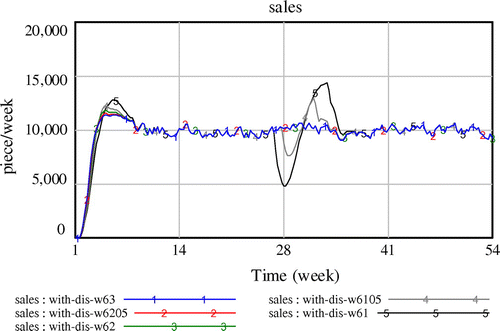
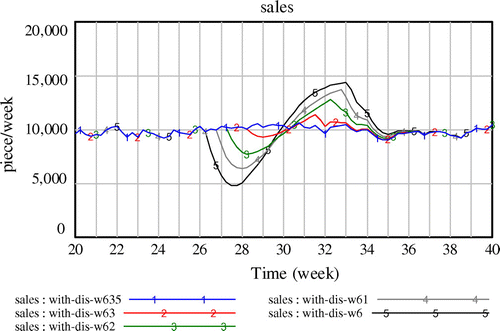
Figure 7 shows the sales with different cover time of wholesaler’s inventory (with six weeks disruption). Herein, cover time of manufacturer’s inventory is 1.5 which has been chosen; cover time of retailer’s inventory = 1.5. In Figure 7, with-dis-w6T1 (T1 = 1, 105, 2, 205 and 3) indicates the simulation results when the cover time of wholesaler’s inventory = 1 (1.5, 2, 2.5 and 3) respectively. Table 4 (Step-2) shows the lowest sales ratio under different combination of inventory level with 6 weeks disruption when cover time of manufacturer’s inventory has been chosen.

Figure 7. Sales with different cover time of wholesaler’s inventory (with 6 weeks disruption).

When the manufacturer and the wholesaler are responsible for 50% and 25% of the sales ratio, the cover time of wholesaler’s inventory should be chosen, so as to let the sales ratio be no less than about 75%. From Figure 7 and Table 4, it can be seen that the choice of cover time of wholesaler’s inventory is 1.5.

4.2.3. Step-3: choosing cover time of retailer’s inventory

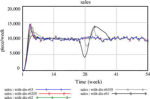
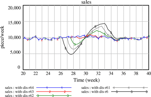
Now, cover time of manufacturer’s inventory and cover time of wholesaler’s inventory have been chosen (1.5 weeks and 1.5 weeks) in terms of the choice rule. Under this situation, the simulation results of sales with production disruption (with-dis-r6T1) are shown in Figure 8. Herein, T1 = 1, 105, 2, 205 and 3 correspond to the cover time of retailer’s inventory = 1, 1.5, 2, 2.5 and 3, respectively. Table 4 (Step-3) shows the lowest sales ratio under different combination of inventory level with six weeks disruption when cover time of manufacturer’s inventory and cover time of wholesaler’s inventory have been chosen.

Figure 8. Sales with different cover time of retailer’s inventory (with 6 weeks disruption).

Similarly, when the manufacturer, the wholesaler and the retailer are responsible for about 50, 25 and 25% of the sales ratio, respectively, the cover time of retailer’s inventory should be chosen so as to let the sales ratio be about 100%. From Figure 8 and Table 4, the choice of cover time of retailer’s inventory is 2 weeks.

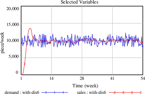
In conclusion, by the choices of cover time of manufacturer’s inventor, cover time of wholesaler’s inventory, and cover time of retailer’s inventory (1.5 weeks, 1.5 weeks and 2 weeks), Figure 9 shows the changes of sales and demand when a six weeks production disruption occurs. It can be seen that the choices can not only ensure 100% sales ratio but also let the sales keep pace with the demand. Namely, the sales fluctuation has disappeared.

Figure 9. Sales and demand with chosen cover time of inventories (with 6 weeks disruption).

4.3. Method for making back-up plans

When a production disruption occurs, as a mitigating method, the manufacturer, the wholesaler or the retailer can back up some products from the contingent suppliers such as other manufacturers, wholesalers or retailers. However, who will make the back-up plan for these products? When and how many to back up? In this model, the periods (k1, k2 and k3) will be decided. At these periods, the supply chain members make back-up plans and choose the adding rates (α1, α2 and α3) for themselves according to their inventory levels. The choice rule for k1 (k2, k3) is that the back-up plan should be carried out at period k1 (k2, k3) when the inventory level decreases to around 50% owing to the disruption. The choice rule for α1, α2 and α3 is that the choice must ensure the sales at the needed sales ratio.

4.3.1. Manufacturer’s choices of k1 and α1

The simulation results of manufacturer’s inventory with a six weeks production disruption (with-dis6T1) are shown in Figure 10. Note that the meaning of with-dis6T1 (T1 = 1, 105, 2, 205 and 3) is the simulation results of Manufacturer’s Inventory when cover time of manufacturer’s inventory = 1 (1.5, 2, 2.5 and 3). Herein, cover time of wholesaler’s inventory = 1 and cover time of retailer’s inventory = 1.5.

Figure 10. Manufacturer’s inventory with different cover time of manufacturer’s inventory (with 6 weeks disruption).

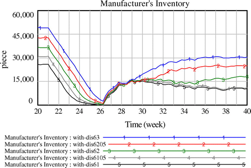
From the consistency point of view, k1 and α1will be analysed and chosen by the simulation result of cover time of manufacturer’s inventory = 1.5.

It’s easy to find that the manufacturer’s inventory decreases to about 50% at the 23rd period (Figure 10). So, 23 is the choice of k1. The Manufacturer’s Inventory equation below is used to simulate the sales with different values of α1.

(3)

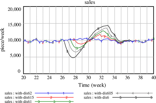
where Mean of Manufacturer’s Inventory is 30358, α1 = 0, 0.5, 1, 1.5 and 2. Figure 11 gives the simulation results of the sales with different α1. Herein, with-dis6T2 (T2 = ‘ ’, 05, 1, 15 and 2) stands for the simulation results of sales when α1 = 0 (0.5, 1, 1.5 and 2). The results show that the manufacturer can achieve 49, 63, 75, 87 and 100% sales ratio when α1 = 0, 0.5, 1, 1.5 and 2, respectively (Table 5).

Figure 11. Sales with different adding rate α1 (with 6 weeks disruption).

Table 5. Choices of the back-up plan makers.

Plan maker and parameters		Choice
Manufacturer	(k1, α1)	(23, 0)	(23, 0.5)	(23, 1)	(23, 1.5)	(23, 2)
	Sales ratio	49%	63%	75%	87%	100%
Wholesaler	(k2, α2)	(25, 0)	(25, 1)	(25, 2)	(25, 3)	(25, 3.5)
	Sales ratio	49%	62%,	77%	91%	100%
Retailer	(k3, α3)	(26, 0)	(26, 1)	(26, 2)	(26, 3)	(26, 4)
	Sales ratio	49%	62%	80%	95%	100%

4.3.2. Wholesaler’s choices of k2 and α2

The wholesaler’s inventory simulation results with a six weeks production disruption are shown in Figure 12. This figure is obtained from the same running as in Figure 10. k2 and α2 will be analysed and chosen by using the simulation result of cover time of manufacturer’s inventory = 1.5.

Figure 12. Wholesaler’s inventory with different cover time of wholesaler’s inventory (with 6 weeks disruption).

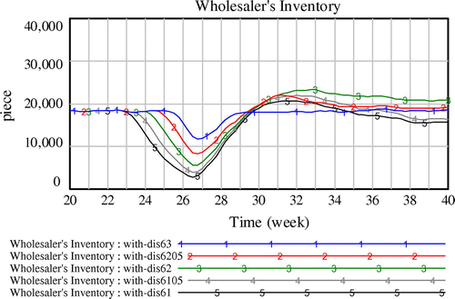
From the simulation results, the wholesaler’s inventory decreases about 50% at the 25th period (Figure 12). So, 25 is the choice of k2. The Wholesaler’s Inventory equation below is used to simulate the sales with different values of α2.(4)

where 17750 is the value of Mean of Wholesaler’s Inventory, α2 = 0, 1, 2, 3 and 3.5. Figure 13 gives the sales simulation results with different α2. with-dis-w6T3 (T3 = ‘ ’, 1, 2, 3 and 35) stands for the simulation results of sales when α2 = 0 (1, 2, 3 and 3.5). The results show that the wholesaler can ensure 49, 62, 77, 91 and 100% sales ratio when α2 = 0, 1, 2, 3and 3.5, respectively (Table 5).

Figure 13. Sales with different adding rate α2 (with 6 weeks disruption).

4.3.3. Retailer’s Choices of k3 and α3

Similarly, the retailer’s inventory simulation results with a six weeks production disruption are shown in Figure 14. Figure 14 is obtained from the same running as in Figure 10. The simulation results of cover time of manufacturer’s inventory = 1.5 are used to analyse and choose k3 and α3.

Figure 14. Retailer’s inventory with different cover time of retailer’s inventory (with 6 weeks disruption).

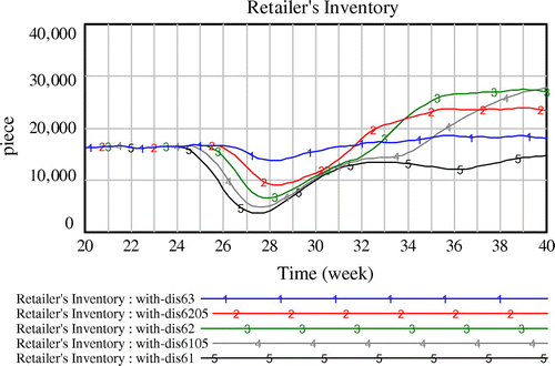
The simulation results show that the retailer’s inventory decreases about 50% at the 26th or the 27th period (Figure 14). So, the choice of k2 is 26. The retailer’s Inventory equation below is used to simulate the sales with different values of α3.(5)

where 15132 is the Mean of retailer’s Inventory, α3 = 0, 1, 2, 3 and 4. Figure 15 gives the sales simulation results with different α3. with-dis-r6T4 (T4 = ‘ ’, 1, 2, 3 and 4) stands for the simulation results for sales when α3 = 0 (1, 2, 3 and 4). The results show that the retailer can ensure about 49, 62, 80, 95 and 100% sales ratio when α3 = 0, 1, 2, 3 and 4, respectively.

Figure 15. Sales with different adding rate α3 (with 6 weeks disruption).

4.3.4. Summary of the choices

The above choices are summarised in Table 5. When a six weeks production disruption occurs, decision-makers can choose the back-up plan based on the needs of sales ratio. For example, if the sales ratio must be larger than 90% so as to maintain the share of consumer market, the back-up plan can be made by the manufacturer, the wholesaler and the retailer:

•	If the back-up plan is made by the manufacturer, the choice must be (k1, α1) = (23, 2). Under this choice, the sales ratio is 100% and the back-up amount is Mean of Manufacturer’s Inventory  × α1 = 30358 × 2 = 60716.
•	If the wholesaler is the plan maker, he has two choices (k2, α2) = (25, 3) and (k2, α2) = (25, 3.5), the sales ratios are 91 and 100%. The amounts of back-up are Mean of Wholesaler’s Inventory  × α2 = 17750 × 3 = 53250 and Mean of Wholesaler’s Inventory  × α2 = 17750 × 3.5 = 62125.
•	If the retailer makes the plan, there are also two choices (k3, α3) = (26, 3) and (k3, α3) = (26, 4), the sales ratios are 95 and 100%. The amounts of back up are Mean of retailer’s Inventory × α3 = 15132 × 3 = 45396 and Mean of retailer’s Inventory × α3 = 15132 × 4 = 60528.

From the economic point of view, when the purchase cost of each back-up product is same for the manufacturer, the wholesaler and the retailer, the choice with lowest back-up amount is the best one. By comparing the above back-up amounts under different choices, the back-up plan should be made by the retailer.

4.4. Effects of the numerical illustration

In Section 4, the numerical examples are used to present the methods of setting multi-echelon inventory levels before the occurring of the disruption and making back-up plans after the production disruption occurs. In a real operation of R/M integrated supply chain, there are a variety of the potential sets of the variables and constants. These examples are certainly not to investigate all possible situations, but they can

•	illustrate the effectiveness of the methods,
•	show how to set the multi-echelon inventory level before the occurring of the disruption step-by-step,
•	show how to make the back-up plans after the production disruption occurs, and
•	present the advantages of the methods given by system dynamics.

5. Sensitivity analysis

In Section 4, in order to ensure the sales at the needed sales ratio, the methods for setting multi-echelon inventory levels before the occurring of the production disruption and making back-up plans after the production disruption occurs are presented. These methods are based on the simulation results in Figure 4(a): the longer the production disruption recovery time is, the larger the sales fluctuation is.

However, do the production disruption and the sales have the same behaviours when some parameters’ values are changed? This problem is investigated by sensitivity analysis. The sets of parameter values for sensitivity analysis are listed in Table 6, including scenarios Sens1, Sens2, Sens3, Sens4 and Sens5. The simulation results are shown in Figure 16. Herein, (sensi)with-disT is the simulation result when the recovery time is T-week (T = 1, 2, 3, 4, 5 and 6) under scenario sensi (i = 1, 2, 3, 4 and 5).

Table 6. Parameter values for sensitivity analysis.

Parameter		Member
		Manufacturer	Wholesaler	Retailer
Sens1	Adjust time of inventory	3.5	3.5	3.5
	Cover time of inventory	1.5	1	1.5
	Lead time	2	1	1.5
Sens2	Adjust time of inventory	3.5	3.5	3.5
	Cover time of inventory	1.5	1	1.5
	Lead time	2.5	1.5	2
Sens3	Adjust time of inventory	2.5	2.5	2.5
	Cover time of inventory	1.5	1	1.5
	Lead time	2	1	1.5
Sens4	Adjust time of inventory	2.5	2.5	2.5
	Cover time of inventory	1.5	1	1.5
	Lead time	2.5	1.5	2
Sens5	Adjust time of inventory	4	3.5	3
	Cover time of inventory	1.5	1	1.5
	Lead time	2	1.5	1

Figure 16. Impacts of different recovery time of production disruption on the sales (r = STEP (0.5, 8)) (under different parameter sets in Sens1, Sens2, Sens3, Sens4 and Sens5). (a) Sales in Sens1, (b) Sales in Sens2, (c) Sales in Sens3, (d) Sales in Sens4, (e) Sales in Sens5.

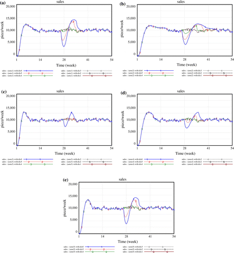
It can be observed from these figures in Figure 16 that the production disruption and the sales have the same behaviours under different value sets. This means the methods for setting multi-echelon inventory levels and making back-up plans are effective in these scenarios.

6. Conclusions

The disruption management of supply chain is very important since the disruption may result in severe consequences. There are two popular strategies of mitigating the disruption: increase the inventory level and back up from other suppliers. In this paper, the new methods are proposed for setting multi-echelon inventory levels and making back-up plans.

In the R/M integrated supply chain, the production disruption of the manufacturer is considered. The Vensim 5.10 is used to create a system dynamics model for the R/M integrated supply chain with production disruption. By the numerical example, the impacts of different recovery time of production disruption on the sales are presented. Based on the simulation results, the methods are given to set multi-echelon inventory levels before the occurring of the production disruption and to make back-up plans after the production disruption occurs, so as to ensure the sales at the needed sales ratio.

We recommend the following research directions. When the market area is destroyed, the sales disruption occurs. How to manage the sales disruption is one interesting topic. Considering the differences between the open form of ‘R/M’ supply chain and the closed-loop form of ‘R/M’ integrated supply chain, how to manage the production disruption in open form of ‘R/M’ supply chain may be the future work.

Disclosure statement

No potential conflict of interest was reported by the authors.

Funding

This work was supported by Humanity and Social Science Planning Foundation of Ministry of Education of China [grant number 15YJA630018], ‘A Group of Five’ Talent Project of the Fund of Tianjin Cultural System, and the Key Advanced Research Project of Tianjin University of Technology and Education [grant number ZDYY1205].

Notes on contributors

Qiaolun Gu is a professor in School of Economics and Management, Tianjin University of Technology and Education. Her research interests include supply chain management, risk control and simulation analysis.

Tiegang Gao is a professor in College of Computer and Control Engineering, Nankai University. His research interests include network optimisation, control theory and information security.

Acknowledgements

The authors would like to thank the reviewers and the editor for comments that significantly improved the paper.

Appendix A.

Variables, constants and equations (Gu and Gao 2012a)

Table

adjust time of collection inventory = 3 Units: week

adjust time of manufacturer’s inventory = 3 Units: week

adjust time of producer’s inventory = 3 Units: week

adjust time of retailer’s inventory = 3 Units: week

adjust time of reusable product inventory = 1 Units: week

adjust time of RMSI = 3 Units: week

‘adjust time of used-product inventory’ = 3 Units: week

adjust time of wholesaler’s inventory = 3 Units: week

Collection Inventory = INTEG (expected collecting rate-purchase rate, 0) Units: piece

collection time = 2 Units: week

coming rate of raw material = expected purchase rate of new material + discrepancy of raw material inventory/adjust time of RMSI Units: kilogram/week

coming rate1 = DELAY FIXED (sales + reusing rate, 7, sales + reusing rate) Units: piece/week

cover time of DCI = 2 Units: week

cover time of DRPI = 1 Units: week

cover time of DUPI = 1.5 Units: week

cover time of manufacturer’s inventory = 2 Units: week

cover time of PPI = 2 Units: week

cover time of retailer’s inventory = 1.5 Units: week

cover time of RMSI = 1.5 Units: week

cover time of wholesaler’s inventory = 1 Units: week

delivery time = 1 Units: week

demand = potential demand market/demand time Units: piece/week

demand backlog = INTEG (demand-demand backlog reduction rate, 0) Units: piece

demand backlog reduction rate = sales Units: piece/week

demand time = 1 Units: week

desired collection inventory = expected purchase rate × cover time of DCI Units: piece

desired manufacturer’s inventory = expected wholesaler’s orders × cover time of manufacturer’s inventory Units: piece

desired part producer’s inventory = expected purchase rate of the new part × cover time of PPI Units: part

desired raw material inventory = expected purchase rate of new material × cover time of RMSI Units: kilogram

desired retailer’s inventory = expected demand × cover time of retailer’s inventory Units: piece

desired reusable product inventory = expected reused product demand rate × cover time of DRPI Units: piece

‘desired used-product inventory’ = ‘expected used-product demand rate’ × cover time of DUPI Units: piece

desired wholesaler’s inventory = expected retailer’s orders × cover time of wholesaler’s inventory Units: piece

disassembly rate = MIN (‘Used-Product will be disassembled’, total amount of the part × r/‘N units (average)’)/disassembly time Units: piece/week

disassembly time = 1.5 Units: week

discrepancy of collection inventory = desired collection inventory − Collection Inventory Units: piece

discrepancy of manufacturer’s inventory = MAX (desired manufacturer’s inventory − Manufacturer’s Inventory, 0) Units: piece

discrepancy of producer’s inventory = MAX (desired part producer’s inventory − Parts Producer’s Inventory, 0) Units: part

discrepancy of raw material inventory = desired raw material inventory − Raw Materials Supplier’s Inventory Units: kilogram

discrepancy of retailer’s inventory = MAX (desired retailer’s inventory-Retailer’s Inventory, 0) Units: piece

discrepancy of reusable product inventory = MAX (desired reusable product inventory - Reusable Product Inventory, 0) Units: piece

‘discrepancy of used-product inventory’ = MAX (‘desired used-product inventory’-‘Used-Product Inventory’, 0) Units: piece

discrepancy of wholesaler’s inventory = MAX (desired wholesaler’s inventory-Wholesaler’s Inventory, 0) Units: piece

expected collecting rate = MIN (expected purchase rate + discrepancy of collection inventory/adjust time of collection inventory, ‘used-product amount’/collection time) Units: piece/week

expected demand = DELAY FIXED (demand, 1, demand) Units: piece/week

expected purchase rate = DELAY FIXED (purchase rate, 1, purchase rate) Units: piece/week

expected purchase rate of new material = DELAY FIXED (purchase rate of new material, 1, purchase rate of new material) Units: kilogram/week

expected purchase rate of the new part = DELAY FIXED (purchase rate of new part, 1, purchase rate of new part) Units: part/week

expected retailer’s orders = DELAY FIXED (retailer’s orders, 1, retailer’s orders) Units: piece/week

expected reused product demand rate = DELAY FIXED (reused product demand rate, 1, reused product demand rate) Units: piece/week

‘expected used-product demand rate’ = DELAY FIXED (remanufacturing rate/‘N units (average)’ + reusing rate, 1, remanufacturing rate/‘N units (average)’ + reusing rate) Units: piece/week

expected wholesaler’s orders = DELAY FIXED (wholesaler’s orders, 1, wholesaler’s orders) Units: piece/week

L units = 3 Units: kilogram/piece

‘M units (average)’ = 40 Units: kilogram/piece

M0 units = 12 Units: kilogram/part

Manufacturer’s Inventory = INTEG (production rate-shipment to wholesaler, 0) Units: piece

material can be recycled = disassembly rate × ‘M units (average)’ Units: kilogram/week

‘N units (average)’ = 3 Units: part/piece

N0 units = 3 Units: part/piece

outing rate = expected collecting rate Units: piece/week

part production rate = expected purchase rate of the new part + discrepancy of producer’s inventory/adjust time of producer’s inventory Units: part/week

parts can be remanufactured = disassembly rate × ‘N units (average)’ Units: part/week

Parts Producer’s Inventory = INTEG (part production rate-purchase rate of new part, 1000) Units: part

potential demand market = 10000 Units: piece

process rate = Remanent Trash/process time Units: kilogram/week

process time = 1 Units: week

product can be reused directly = MIN (reusable product should satisfy, ‘Used-Product Inventory’ × reusing percentage)/testing time Units: piece/week

product can’t be reused directly = ‘Used-Product Inventory’ × (1-reusing percentage)/testing time Units: piece/week

production rate = expected wholesaler’s orders + discrepancy of manufacturer’s inventory/adjust time of manufacturer’s inventory Units: piece/week

production time = 2 Units: week

production time of new part = 1.5 Units: week

purchase rate = ‘used-product should satisfy’/purchase time Units: piece/week

purchase rate of new material = (total amount of the material-recycling rate × recycling time)/purchase time of new material Units: kilogram/week

purchase rate of new part = (total amount of the part-remanufacturing rate × remanufacturing time)/purchase time of new part Units: part/week

purchase time = 2 Units: week

purchase time of new material = 1.5 Units: week

purchase time of new part = 2 Units: week

Raw Materials Supplier’s Inventory = INTEG (coming rate of raw material-purchase rate of new material, 100000) Units: kilogram

Recyclable Material Inventory = INTEG (material can be recycled-recycling rate, 0) Units: kilogram

recycling rate = MIN (Recyclable Material Inventory, total amount of the material)/recycling time Units: kilogram/week

recycling time = 1 Units: week

Remanent Trash = INTEG (remanent trash will be disposed-process rate, 0) Units: kilogram

remanent trash will be disposed = disassembly rate × L units Units: kilogram/week

Remanufacturable Part Inventory = INTEG (parts can be remanufactured-remanufacturing rate, 0) Units: part

remanufacturing rate = MAX (Remanufacturable Part Inventory, total amount of the part × r)/remanufacturing time Units: part/week

remanufacturing time = 2 Units: week

Retailer’s Inventory = INTEG (shipment to retailer-sales, 0) Units: piece

retailer’s orders = expected demand + discrepancy of retailer’s inventory/adjust time of retailer’s inventory Units: piece/week

retailer’s orders backlog = INTEG (retailer’s orders-retailer’s orders reduction rate, 0) Units: piece

retailer’s orders reduction rate = shipment to retailer Units: piece/week

Reusable Product Inventory = INTEG (product can be reused directly-reusing rate, 0) Units: piece

reusable product should satisfy = INTEG (should satisfy rate of reusable product - satisfied rate of reusable product, 0) Units: piece

reused product demand = INTEG (reused product demand rate-satisfied rate of reused product, 0) Units: piece

reused product demand rate = 20 Units: piece/week

reusing percentage = 0.2 Units: Dmnl

reusing rate = MIN (reused product demand, Reusable Product Inventory)/reusing time Units: piece/week

reusing time = 2 Units: week

sales = MIN (Retailer’s Inventory, demand backlog)/delivery time Units: piece/week

satisfied rate of reusable product = product can be reused directly Units: piece/week

satisfied rate of reused product = reusing rate Units: piece/week

‘satisfied rate of used-product’ = purchase rate Units: piece/week

shipment time to retailer = 1.5 Units: week

shipment time to wholesaler = 1 Units: week

shipment to retailer = MIN (Wholesaler’s Inventory, retailer’s orders backlog)/shipment time to retailer Units: piece/week

shipment to wholesaler = MIN (Manufacturer’s Inventory, wholesaler’s orders backlog)/shipment time to wholesaler Units: piece/week

should satisfy rate of reusable product = expected reused product demand rate + discrepancy of reusable product inventory/adjust time of reusable product inventory Units: piece/week

‘should satisfy rate of used-product’ = ‘expected used-product demand rate’ + ‘discrepancy of used-product inventory’/‘adjust time of used-product inventory’ Units: piece/week

testing time = 1 Units: week

total amount of the material = part production rate × production time of new part × M0 units Units: kilogram

total amount of the part = production rate × production time × N0 units Units: part

‘used-product amount’ = INTEG (coming rate1-outing rate, 0) Units: piece

‘Used-Product Inventory’ = INTEG (purchase rate-product can be reused directly-product can’t be reused directly, 0) Units: piece

‘used-product should satisfy’ = INTEG (‘should satisfy rate of used-product’ - ‘satisfied rate of used-product’, 0) Units: piece

‘Used-Product will be disassembled’ = INTEG ((product can’t be reused directly-disassembly rate) × 1,0) Units: piece

Wholesaler’s Inventory = INTEG (shipment to wholesaler-shipment to retailer,0) Units: piece

wholesaler’s orders = expected retailer’s orders + discrepancy of wholesaler’s inventory/adjust time of wholesaler’s inventory Units: piece/week

wholesaler’s orders backlog = INTEG (wholesaler’s orders-wholesaler’s orders reduction rate, 0) Units: piece

wholesaler’s orders reduction rate = shipment to wholesaler Units: piece/week

References

- Cauvin, A. C. A., A. F. A. Ferrarini, and E. T. E. Tranvouez. 2009. “Disruption Management in Distributed Enterprises: A Multi-agent Modelling and Simulation of Cooperative Recovery Behaviours.” International Journal of Production Economics 122 (1): 429–439.10.1016/j.ijpe.2009.06.014
- Chen, K. B., and T. J. Xiao. 2009. “Demand Disruption and Coordination of the Supply Chain with a Dominant Retailer.” European Journal of Operational Research 197 (1): 225–234.10.1016/j.ejor.2008.06.006
- Chen, J. X., G. H. Li, and G. H. Shi. 2011. “Supply Chain System Dynamics Simulation with Disruption Risks.” Industrial Engineering and Management 16 (6): 35–41.
- Georgiadis, P., and M. Besiou. 2008. “Sustainability in Electrical and Electronic Equipment Closed-loop Supply Chains: A System Dynamics Approach.” Journal of Cleaner Production 16 (15): 1665–1678.10.1016/j.jclepro.2008.04.019
- Gu, Q. L., and T. G. Gao. 2012a. “Joint Decisions for R/M Integrated Supply Chain Using System Dynamics Methodology.” International Journal of Production Research 50 (16): 4444–4461.10.1080/00207543.2011.600344
- Gu, Q. L., and T. G. Gao. 2012b. “Managing Supply Disruption for Remanufacturer of Reverse Supply Chain.” Proceedings of 2012 IEEE International Conference on Service Operations and Logistics, and Informatics, Suzhou, China, July. 331–335.10.1109/SOLI.2012.6273557
- Gu, Q. L., G. Tagaras, and T. G. Gao. 2014. “Disruption Risk Management in Reverse Supply Chain by Using System Dynamics.” Proceedings of the 2014 International Conference on Management Science and Management Innovation, Changsha, China, June. 512–517.
- Jain, A. 2010. Impact of Supply Uncertainty in Supply Chain. Saarbrücken: LAP Lambert Academic Publishing AG & Co KG.
- Latour, A. 2001. “Trial by Fire: A Blaze in Albuquerque Sets Off Major Crisis for Cell Phone Giants.” The Wall Street Journal 2001, A1.
- Li, X., and Y. Chen. 2010. “Impacts of Supply Disruptions and Customer Differentiation on a Partial-backordering Inventory System.” Simulation Modelling Practice and Theory 18 (5): 547–557.10.1016/j.simpat.2009.12.010
- Lorentz, H., and O. P. Hilmola. 2012. “Confidence and Supply Chain Disruptions: Insights into Managerial Decision-making from the Perspective of Policy.” Journal of Modelling in Management 7 (3): 328–356.10.1108/17465661211283304
- Papachristos, G. 2014. “Transition Inertia Due to Competition in Supply Chains with Remanufacturing and Recycling: A Systems Dynamics Model.” Environmental Innovation and Societal Transitions 12: 47–65. doi:10.1016/j.eist.2014.01.005.
- Qi, X. T., J. F. Bard, and G. Yu. 2004. “Supply Chain Coordination with Demand Disruptions.” Omega 32 (4): 301–312.10.1016/j.omega.2003.12.002
- Rice, J., and F. Caniato. 2003. “Building a Secure and Resilient Supply Chain.” Supply Chain Management Review 7 (5): 22–30.
- Vlachos, D., P. Georgiadis, and E. Iakovou. 2007. “A System Dynamics Model for Dynamic Capacity Planning of Remanufacturing in Closed-loop Supply Chains.” Computers & Operations Research 34 (2): 367–394.10.1016/j.cor.2005.03.005
- Wilson, M. C. 2007. “The Impact of Transportation Disruptions on Supply Chain Performance.” Transportation Research Part E: Logistics and Transportation Review 43 (4): 295–320.10.1016/j.tre.2005.09.008
- Wang, Y. X., X. Y. Chang, Z. G. Chen, Y. G. Zhong, and T. J. Fan. 2014. “Impact of Subsidy Policies on Recycling and Remanufacturing Using System Dynamics Methodology: A Case of Auto Parts in China.” Journal of Cleaner Production 74 (7): 161–171.10.1016/j.jclepro.2014.03.023
- Xia, Y. S., T. J. Xiao, and G. Yu. 2004. “Production and Inventory Management with Raw Material Supply Disruptions.” Working paper. Austin, TX: McCombs School of Business, The University of Texas at Austin.
- Xiao, T. J., and G. Yu. 2006. “Supply Chain Disruption Management and Evolutionarily Stable Strategies of Retailers in the Quantity-setting Duopoly Situation with Homogeneous Goods.” European Journal of Operational Research 173 (2): 648–668.10.1016/j.ejor.2005.02.076
- Xiao, T. J., and X. T. Qi. 2008. “Price Competition, Cost and Demand Disruptions and Coordination of a Supply Chain with One Manufacturer and Two Competing Retailers.” Omega 36 (5): 741–753.10.1016/j.omega.2006.02.008
- Yang, J., X. T. Qi, and G. Yu. 2005. “Disruption Management in Production Planning.” Naval Research Logistics 52 (5): 420–442.10.1002/(ISSN)1520-6750
- Yu, H. S., A. Z. Zeng, and L. D. Zhao. 2009. “Single or Dual Sourcing: Decision-making in the Presence of Supply Chain Disruption Risks.” Omega 37 (4): 788–800.10.1016/j.omega.2008.05.006