An integrated methodology for the used product selection problem faced by third-party reverse logistics providers

Abstract

The rise of electronic commerce and the stricter government regulations on the recovery of end-of-life products increased the number of products returned by customers. A company may deal with increasing product returns by developing its own reverse logistic system. However, high fixed costs associated with dedicated reverse logistics equipment and infrastructure force many companies to outsource their reverse logistics operations to third-party reverse logistics providers. One of the important problems faced by third-party reverse logistics providers is the selection of the types of used products to be collected. In this study, a four-phase used product selection methodology is proposed. First, the quantitative and qualitative selection criteria are determined. Then the weights of the criteria are calculated using fuzzy analytic hierarchy process. Next, simulation models are employed to determine the values of quantitative criteria. Finally, technique for order preference by similarity to ideal solution ranks alternative used product types. A numerical example is also provided in order to present the applicability of the proposed methodology.

Keywords:

• Third-party reverse logistics provider
• used product
• fuzzy AHP
• TOPSIS
• simulation

1. Introduction

Dramatic decrease in natural resources and suitable landfill areas has forced many governments to impose strict environmental regulations on manufacturers. According to some of these regulations, manufacturers have to take back their products at the end of their useful life. In addition to environmental regulations, more liberal return policies and rise in the volume of internet marketing have contributed to the increase in customer returns. In order to deal with increasing customer returns, firms invest in reverse logistics (RL) which involves all the activities associated with the collection and either recovery or disposal of returned products (Ilgin and Gupta 2013).

Reverse logistics requires the establishment of collection and product recovery facilities. In each facility, sophisticated material handling equipment must be used and a dedicated workforce is required for the maintenance and daily operation of the facilities. Due to the high level of uncertainty associated with the collection and recovery of returned products, planning of reverse logistics operations cannot be carried out using the existing forward logistics planning system. In order to avoid the high fixed costs and planning complexities, many companies outsource their reverse logistics operations to third-party reverse logistics providers (3PRLPs) (Shaharudin, Zailani, and Ismail 2014).

Due to the increasing importance of 3PRLPs in reverse logistics, the number of studies on 3PRLPs is on the rise (Ilgin, Gupta, and Battaïa 2015). The majority of these studies focus on the evaluation and selection of 3PRLPs. They try to help companies find a suitable 3PRLP based on the consideration of various economic and environmental criteria. There are several studies focusing on the design of reverse logistic networks for 3PRLPs (Ko and Evans 2007; Lee, Bian, and Dong 2007a; Min and Ko 2008). However, the research on the determination of the most suitable used product to be processed by a 3PRLP is very limited (Pochampally and Gupta 2008). In order to fill this gap, this study proposes a solution methodology for the used product selection problem faced by many 3PRLPs.

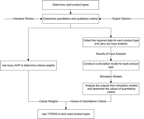
The proposed used product selection methodology involves four stages. The first stage involves the determination of alternative used products and quantitative and qualitative evaluation criteria. Criteria weights are calculated using fuzzy AHP in the second stage. Numerical values of quantitative criteria are calculated in the third stage by constructing simulation models for each product type. Finally, used product types are ranked using Technique for Order Preference by Similarity to Ideal Solution (TOPSIS) based on quantitative and qualitative criteria.

The remainder of the paper is organised as follows. Section 2 presents a literature review on the issues considered in the paper. Brief information on the techniques used in the proposed methodology is provided in Section 3. Section 4 discusses the details of the proposed methodology. A numerical example is presented in Section 5. Finally, Section 6 concludes the paper.

2. Literature review

In recent years, researchers have studied various aspects of reverse logistics due to the increasing importance of RL operations in environmental and economic performance of companies. The most widely used RL issues include network design (Barker and Zabinsky 2008), product acquisition management (Nikolaidis 2009), selection of third-party reverse logistic providers (Efendigil, Önüt, and Kongar 2008) and recovery of used products (Rahimifard et al. 2009). We refer the interested reader to Ilgin and Gupta (2010), Sasikumar and Kannan (2008a, 2008b, 2009) and Govindan, Soleimani, and Kannan (2015) for a comprehensive review of issues associated with RL.

The majority of the studies on 3PRLPs try to determine the most suitable 3PRLP by considering various environmental and economic criteria. Multi-criteria decision-making techniques are commonly used in these studies. Meade and Sarkis (2002) developed an analytic network process (ANP)-based methodology for the evaluation and selection of 3PRLPs providers. Govindan, Sarkis, and Palaniappan (2013) first used analytic hierarchy process (AHP) to identify the most prioritised 3PRLP selection criteria. Then, they employed ANP in order to determine the most suitable reverse logistic provider. Saen (2010, 2011) and Azadi and Saen (2011) proposed data envelopment analysis (DEA)-based solution methodologies for 3PRLP selection problem. Kannan, Pokharel, and Sasi Kumar (2009) selected the best 3PRLP by integrating interpretive structural modelling and fuzzy TOPSIS. Efendigil, Önüt, and Kongar (2008) integrated fuzzy AHP and artificial neural networks.

There are several papers analysing the network design problem faced by 3PRLPs. Suyabatmaz, Altekin, and Şahin (2014) developed hybrid simulation-analytical modelling approaches for the RL network design of a 3PRLP. The closed-loop supply chain network design model proposed by Lee, Bian, and Dong (2007a) has two objectives: maximisation of returned products shipped from customers back to the collection facilities and minimisation of the total costs associated with the forward and reverse logistics operations. First, fuzzy goal programming is used to develop a compromised solution. Then, a genetic algorithm (GA) is employed to solve the problem. Lee, Bian, and Dong (2007b) developed a GA-based solution methodology for the mixed integer linear programming model associated with the closed loop supply chain network design problem of a 3PRLP.

Although selection of suitable used products is an important problem faced by 3PRLPs, the research on this area is very limited. Pochampally and Gupta (2008) proposed a fuzzy cost–benefit function (FCBF)-based used product selection methodology. An FCBF value is calculated for each used product by taking the ratio of equivalent value of revenues to the equivalent value of costs. Fuzzy numbers are used to model the uncertainty associated with three parameters (viz., supply of used products, probability of missing component and probability of bad quality component). It is assumed that disassembly times are constant and the disassembled components are reused immediately. In addition, the qualitative criteria associated with the selection of used products are not considered in this study.

This study extends the used product selection methodology proposed by Pochampally and Gupta (2008) in three ways. First, stochastic disassembly times and stochastic demand for the disassembled components are considered. Second, holding and backorder costs are taken into consideration while calculating the total cost. Third, in addition to quantitative criteria, several qualitative used product selection criteria are included in the proposed methodology.

3. Techniques used

The following techniques employed in the proposed methodology are introduced in this section: discrete event simulation (DES) (Section 3.1), fuzzy logic and fuzzy AHP (Section 3.2) and TOPSIS (Section 3.3).

3.1. Discrete event simulation

DES, a powerful tool used in the analysis of complex processes or systems, analyzes the behaviour of a real-world system by developing a model of it. This model can be used to test new policies, decision rules, information flows and operating procedures without disrupting the operations of the existing system. Contrary to the continuous simulation, state variables in DES change instantaneously at discrete points in time. The interested reader is referred to well-known texts for more information on DES (Banks et al. 2001; Law 2007).

A programming language (e.g. Delphi, C++) or a simulation package (e.g. Arena, Promodel) can be employed to build a DES model. The DES models presented in this paper were constructed using Arena simulation package (Kelton, Sadowski, and Sadowski 2007).

3.2. Fuzzy logic and fuzzy AHP

The analytical hierarchy process (AHP) introduced by Saaty (Saaty 1980) is a frequently used multi-criteria decision-making methodology. It defines the decision problem as a hierarchy consisting of the goal, criteria and alternatives. The expert judgements are used to carry out pairwise comparisons among criteria and alternatives. It has the ability of considering tangible as well as intangible criteria. However, there are two main limitations of AHP: use of unbalanced scale of judgements and its inability to adequately handle the inherent uncertainty and imprecision in the pairwise comparison process. These limitations can be overcome using fuzzy AHP which integrates AHP with the concepts of fuzzy set theory. The following subsections present brief information on fuzzy logic and fuzzy AHP.

3.2.1. Fuzzy sets and fuzzy numbers

Fuzzy logic (FL) was developed by Zadeh (Zadeh 1965) as an extension of Boolean logic. While there are two truth values (viz., true (1) and false (0)) in Boolean logic, FL can model partial truth values by considering the whole interval between 0 (False) and 1 (True). It uses fuzzy sets to quantify the uncertainty in human judgement. We can define a fuzzy set as follows:

(1)

where X is a space of points, A is a fuzzy set defined in X and f_A(x) is a membership function which associates with each point in X a real number in the interval [0,1]. The membership function f_A(x) indicates the degree of membership of x in A. There are many different forms of membership functions used to define fuzzy numbers. Triangular fuzzy number (TFN) depicted in Figure 1 is the most commonly used fuzzy number.

Figure 1. Triangular fuzzy number.

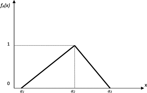
Equation 2 presents the membership function of a TFN.(2)

A technique called ‘defuzzification’ can be used to convert a fuzzy number into a crisp real number. Defuzzification can be achieved using one of the several defuzzification methods. For instance, defuzzification of a TFN into a crisp real number (Q) using the centre of area method can be expressed as follows (Ilgin and Gupta 2012):(3)

The five basic operations on TFNs (Chan, Chan, and Chan 2003; Tsaur, Chang, and Yen 2002) can be expressed as follows (A = (a₁, a₂, a₃) and B = (b₁, b₂, b₃)):(4) (5) (6) (7) (8)

3.2.2. Extent analysis on fuzzy AHP

There are various solution methodologies developed for fuzzy AHP (van Laarhoven and Pedrycz 1983; Buckley 1985; Chang 1996). Chang’s extent analysis (Chang 1996) employed in this study is commonly used by researchers since this method is relatively easier than the other approaches. Let X =  be a set of an object and U =  be a goal set. According to the extent analysis method, an object is taken and extent analysis for each goal, g_i is performed. Therefore, m number of extent analysis values for each object can be obtained, with the following symbols:(9)

where all the are TFNs.

The steps of the Chang’s extent analysis can be defined as follows:

Step 1: The value of fuzzy synthetic extent associated with the object i is defined as follows:(10)

where  represents fuzzy multiplication and superscripts −1 represents the fuzzy inverse.

The fuzzy addition operation of m extent analysis values for a given matrix is performed in order to calculate as follows:(11)

and in order to obtain the value of , first the fuzzy addition operation of values is performed:(12)

and then the inverse of the vector in Equation 12(12) is computed:(13)

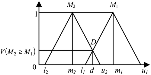
Step 2: The degree of possibility of M₂ = (l₂, m₂, u₂) ≥ M₁ = (l₁, m₁, u₁) is defined as follows:(14)

and it can be equivalently expressed as follows:(15) (16)

where d is, as shown in Figure 2, the ordinate of the highest intersection point D between and . The values of both V(M₁ ≥ M₂) and V(M₂ ≥ M₁) must be calculated in order to compare M₁ and M₂.

Figure 2. Intersection point between M₁ and M₂.

Step 3: The degree of possibility for a convex fuzzy number to be greater than k convex fuzzy numbers M_i(i = 1, 2, …, k) can be defined by:(17)

Assuming that , the weight vector is given by:(18)

Step 4: Through normalisation, the normalised weight vectors are obtained:(19)

where W is a non-fuzzy number.

3.3. TOPSIS

TOPSIS (The Technique for Order Preferences by Similarity to an Ideal Solution) is a multi-criteria decision-making technique trying to determine the best alternative based on the concepts of compromise solution. According to this method, the chosen alternative should have the shortest Euclidian distance from the ideal solution and the greatest Euclidean distance from the negative-ideal solution (Hwang and Yoon 1981). The decision-maker creates a decision matrix (A = (a_ij)_m×n) which consists of m alternatives, n criteria and the rating of each alternative with respect to each criterion. Following the construction of the decision matrix, the following steps are followed in TOPSIS (Triantaphyllou and Lin 1996):

Step 1: Construct the normalised decision matrix via the following equation:(20)

Step 2: Establish the weighted normalized decision matrix (V = (v_ij)_m×n) as follows:(21)

where w_j is the weight of criterion j.

Step 3: Use the weighted normalized decision matrix to determine the ideal (A^*) and negative-ideal (A⁻) solutions:(22) (23)

where J and J^′ represent the benefit and cost criteria, respectively.

Step 4: Calculate the Euclidean distances of each alternative from A^* and A⁻ as follows:(24) (25)

Step 5: Derive the relative closeness coefficient of each alternative as follows:(26)

Step 6: Rank the alternatives according to their relative closeness coefficient values. Recommend the alternative with the highest C^* value as the best alternative.

4. The proposed methodology

The outline of the proposed methodology is presented in Figure 3. First, the used product types and the quantitative and qualitative evaluation criteria are determined. Next, criteria weights are calculated using fuzzy AHP and simulation models built for each product type are employed to calculate the numerical values of quantitative criteria. Finally, used product types are ranked using TOPSIS based on quantitative and qualitative criteria.

Figure 3. Flow chart of the proposed methodology.

The following section presents a numerical example in order to illustrate the practical use of the proposed methodology.

5. Numerical example

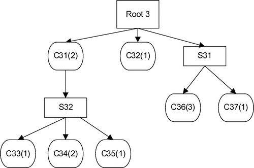
The proposed methodology is illustrated by presenting a numerical example. Three products are considered in the example. The product structures are presented in Figures 4–6. In these figures, S represents subassembly and C represents component. For instance, S₂₁ is the first subassembly of product 2 and C₃₂ is the second component of product 3. The numbers in parentheses represent the multiplicity of each component. For instance C₁₁₍₂₎ means that there are two type 1 components in product 1.

Figure 4. Structure of product 1.

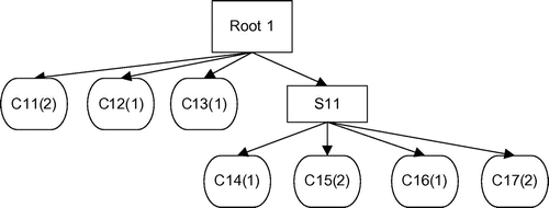
Figure 5. Structure of product 2.

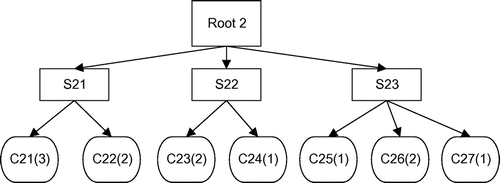
Figure 6. Structure of product 3.

5.1. Determination of evaluation criteria

The following subsections present information on the quantitative and qualitative criteria for the evaluation of used product alternatives.

5.1.1. Quantitative criteria

There are two quantitative criteria: Total Revenue and Total Cost. Numerical values of both criteria for each product type are calculated using a separate simulation model. The following subsections present the mathematical expressions employed by the simulation model for the calculation of different components of total revenue and total cost.

5.1.1.1. Total revenue

Total revenue (TR) for each product is calculated by summing total reuse revenue and total recycle revenue.

Total reuse revenue (R_reuse) is calculated as follows:(27)

where N is the number of component types in the product, RU_j is the total number of reusable component j disassembled during the simulated time period and RV_j is the resale value of reusable component type j ($).

Total recycle revenue (R_recycle) is calculated as follows:(28)

where N is the number of component types in the product, RC_j is the total number of non-usable component j disassembled during the simulated time period, RCP_j is the recyclable content of component j, W_j is the weight of component j (kg) and URR_j is the unit recycling revenue of component j ($/kg).

5.1.1.2. Total cost

Total cost (TC) for each product is calculated by summing total collection cost, total disposal cost, total reprocessing cost, total holding cost and total backorder cost.

Total collection cost (C_collection) is calculated as follows:(29)

where TP is the total number of products collected during the simulated time period and UCC is the unit collection cost ($/product).

Total disposal cost (C_disposal) is calculated as follows:(30)

where N is the number of component types in the product, RC_j is the total number of non-usable component j disassembled during the simulated time period, RCP_j is the recyclable content of component j, W_j is the weight of component j (kg) and UDC_j is the unit disposal cost of component j ($/kg).

Total reprocessing cost (C_reprocessing) is calculated as follows:(31)

where TD is the total number of products disassembled during the simulated time period, DT is the total disassembly time of the product and UDC is the unit disassembly cost ($/minute).

It must be noted that probability of breakage (pb_j) and probability of a missing component (pm_j) are considered while determining whether a component is usable or non-usable. Probability of missing component is the probability that the product does not involve the component. Probability of breakage is the probability that the disassembled component is defective.

Total holding cost (C_holding) is calculated as follows:(32)

where N is the number of component types in the product and H_j is the holding cost of component j during the simulated time period. Holding cost is calculated by considering the price of the component, holding cost rate and the changes in the inventory level of the component during the simulated time period. Holding cost rate is taken as 0.20 for all component types.

Total backorder cost (C_backorder) is calculated as follows:(33)

where N is the number of component types in the product and B_j is the cost of backorders associated with component j during the simulated time period. Backorder cost is calculated by considering the price of the component, backorder cost rate and the changes in the backorder level of the component during the simulated time period. Backorder cost rate is taken as 0.40 for all component types.

It must be noted that total cost and total revenue can be calculated using different cost and revenue components. For instance, if refurbishment and/or remanufacturing-related revenues are possible in reverse logistic systems, those revenue components must also be considered while calculating total revenue. Total cost of this system must be calculated by considering refurbishment/remanufacturing-related cost components.

5.1.2. Qualitative criteria

The following qualitative criteria should also be considered by the 3PRLP:

•	The level of prior experience on the disassembly of the product (EXP): The 3PRLP would prefer a product which has similar characteristics with the products previously disassembled by the 3PRLP. This will increase the possibility of using existing workforce and logistics infrastructure. If the product’s structure is very different from the products that were disassembled by the 3PRLP in the past, 3PRLP may need to hire additional workers with different skills. In addition, the size and capacity of the material handling equipment and vehicles may not be suitable for the handling of the products, subassemblies and components.
•	The level of disassembly line modification required by the product (MOD): The product which requires less modification on the number of workstations and type of disassembly tools will be more attractive for the 3PRLP. If the precedence relations among components of the product are different from the products previously disassembled by the 3PRLP, the disassembly line must be redesigned by changing the location of workstations. Additional disassembly tools may also be added, especially if the product involves fasteners new to the 3PRLP.
•	The ease of finding Original Equipment Manufacturers (OEMs) willing to work with 3PRLP for the recovery of the product (EAS): The 3PRLP will have a smoother supply of used products if the product is produced by many OEMs. If the product is produced in limited quantities by few OEMs, the 3PRLP may have difficulty in finding sufficient number of used products. This situation negatively affects the profitability of the third-party reverse logistics system operated by the 3PRLP.

5.2. Determination of criteria weights using fuzzy AHP

Fuzzy AHP based on Chang’s extent analysis is used to determine the weights of used product selection criteria determined in Section 5.1. Linguistic weight conversion scale is provided in Table 1. Table 2 presents the comparative importance values of the criteria. Table 3 was obtained by converting the linguistic preferences of Table 2 into TFNs based on the conversion scale.

Table 1. Linguistic weight conversion scale.

Linguistic scale	Fuzzy triangular scale	Reciprocal fuzzy triangular scale
Equally preferred (E)	(1, 1, 1)	(1, 1, 1)
Moderately preferred (M)	(2/3, 1, 3/2)	(2/3, 1, 3/2)
Strongly preferred (S)	(3/2, 2, 5/2)	(2/5, 1/2, 2/3)
Very strongly preferred (VS)	(5/2, 3, 7/2)	(2/7, 1/3, 2/5)
Absolutely preferred (A)	(7/2, 4, 9/2)	(2/9, 1/4, 2/7)

Table 2. Comparative importance values of criteria.

	TC	TR	EXP	MOD	EAS
TC	E	M	S	M	S
TR	1/M	E	M	M	M
EXP	1/S	1/M	E	E	S
MOD	1/M	1/M	1/E	E	M
EAS	1/S	1/M	1/S	1/M	E

Table 3. Comparative importance values of criteria converted into TFNs.

	TC	TR	EXP	MOD	EAS
TC	(1, 1, 1)	(2/3, 1, 3/2)	(3/2, 2, 5/2)	(2/3, 1, 3/2)	(3/2, 2, 5/2)
TR	(2/3, 1, 3/2)	(1, 1, 1)	(2/3, 1, 3/2)	(2/3, 1, 3/2)	(2/3, 1, 3/2)
EXP	(2/5, 1/2, 2/3)	(2/3, 1, 3/2)	(1, 1, 1)	(1, 1, 1)	(3/2, 2, 5/2)
MOD	(2/3, 1, 3/2)	(2/3, 1, 3/2)	(1, 1, 1)	(1, 1, 1)	(2/3, 1, 3/2)
EAS	(2/5, 1/2, 2/3)	(2/3, 1, 3/2)	(2/5,1/2,2/3)	(2/3,1,3/2)	(1, 1, 1)

Criteria weights were obtained by applying the four steps of Chang’s extent method to Table 3 as follows:

Step 1: For each criterion, the value of fuzzy synthetic extent (S_i) was computed using Equations 10(10) –13(13) :

Step 2: V (M₂ ≥ M₁) value was computed for each criterion using Equations 14(14) –16(16) :

Step 3: Equations 17(17) and 18(18) were used to determine the weight vector:

Step 4: The normalised weight vector is obtained via normalisation:

5.3. Calculation of the expected values of the quantitative criteria using simulation

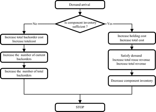
The expected values of quantitative selection criteria were calculated using simulation models of the alternative used products. Arena 14.0 was used to construct all simulation models. Figure 7 presents the flow chart of the operations performed following the disassembly of a component. The flow chart of the operations performed for the satisfaction of component demand is depicted in Figure 8.

Figure 7. Flow chart of the operations performed following the disassembly of a component.

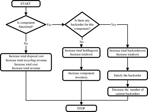
Figure 8. Flow chart of the operations performed for the satisfaction of component demand.

Component characteristics are presented in Tables 4–6. The inter-arrival times of Product 1, Product 2 and Product 3 are assumed to be distributed exponentially with the means of 60, 25 and 30 min, respectively. Unit collection costs of Product 1, Product 2 and Product 3 are $20, $18 and $23, respectively. Demand inter-arrival times are exponentially distributed with the means (in minutes) presented in the last columns of Tables 4–6. Disassembly times of roots and subassemblies are assumed to be distributed exponentially with the means (in minutes) presented in Table 7. Unit disassembly cost was taken as $1/minute, while the holding and backorder cost rates were taken as 5 and 30%, respectively. It must be noted that the fuzzy pb_j and pm_j values were defuzzified using Equation 3(3) and the resulting crisp values were used in the simulation models.

Table 4. Component characteristics for used product 1.

Component	RVj	Wj	RCPj (%)	URRj	UDCj	pbj	pmj	Mean demand inter-arrival time
C11	18	3.5	30	0.5	0.30	(0.2, 0.3, 0.4)	(0.1, 0.1, 0.2)	10
C12	24	2	40	1	0.60	(0.1, 0.1, 0.2)	(0.3, 0.4, 0.5)	7
C13	20	2	70	0.5	0.25	(0.1, 0.2, 0.3)	(0.1, 0.1, 0.2)	7
C14	25	1	90	2	0.75	(0.2, 0.3, 0.4)	(0.1, 0.2, 0.3)	12
C15	14	3	60	1.5	1.00	(0.1, 0.1, 0.2)	(0.2, 0.3, 0.4)	9
C16	12	4	70	1	0.50	(0.1, 0.2, 0.3)	(0.1, 0.2, 0.2)	8
C17	19	4	70	1	0.50	(0.1, 0.1, 0.2)	(0.1, 0.1, 0.2)	12

Table 5. Component characteristics for used product 2.

Component	RVj	Wj	RCPj (%)	URRj	UDCj	pbj	pmj	Mean demand inter-arrival time
C21	15	5	50	2	0.25	(0.1, 0.2, 0.3)	(0.2, 0.2, 0.3)	10
C22	26	3	70	2.5	0.75	(0.1, 0.1, 0.2)	(0.3, 0.4, 0.5)	12
C23	18	2	40	2.5	0.35	(0.1, 0.1, 0.2)	(0.2, 0.2, 0.3)	5
C24	20	5	80	1	0.60	(0.1, 0.2, 0.2)	(0.2, 0.3, 0.4)	13
C25	10	1	80	0.5	0.25	(0.2, 0.3, 0.4)	(0.3, 0.3, 0.4)	10
C26	9	2	90	0.5	0.30	(0.1, 0.2, 0.3)	(0.1, 0.2, 0.3)	10
C27	25	2	50	1	0.40	(0.1, 0.1 ,0.2)	(0.3, 0.4, 0.4)	9

Table 6. Component characteristics for used product 3.

Component	RVj	Wj	RCPj (%)	URRj	UDCj	pbj	pmj	Mean demand inter-arrival time
C31	10	4.5	60	2	0.50	(0.2, 0.2, 0.3)	(0.0, 0.1, 0.1)	8
C32	20	4	50	3	1.00	(0.1, 0.1, 0.2)	(0.1, 0.2, 0.3)	10
C33	15	1	80	1	0.75	(0.1, 0.2, 0.3)	(0.3, 0.4, 0.4)	9
C34	25	2	70	0.5	0.75	(0.1, 0.1, 0.2)	(0.0, 0.1, 0.1)	10
C35	12	3	80	1	1.25	(0.2, 0.3, 0.4)	(0.3, 0.4, 0.4)	8
C36	12	4	50	1	0.50	(0.1, 0.2, 0.3)	(0.1, 0.1, 0.2)	12
C37	25	4	90	2	1.00	(0.1, 0.1, 0.2)	(0.1, 0.1, 0.2)	7

Table 7. Mean disassembly times of roots and subassemblies.

Product	Subassembly	Mean disassembly time
1	Root	5
	S11	3
2	Root	10
	S21	3
	S22	2
	S23	3
3	Root	5
	S31	4
	S32	5

The simulation models were run for 120,960 min, the equivalent of 1 year with one 8-h shift per day. The models were replicated 50 times and the warm-up period was taken as 15,000 min. Average total revenue and total cost values for each product type are presented in Table 8.

Table 8. Average total revenue and average total cost values for each product type.

	Product 1	Product 2	Product 3
Total Revenue	228,460	561,690	627,450
Total Cost	294,680	346,020	176,800

5.4. Evaluation of used products using TOPSIS

The last stage of the proposed methodology involves the ranking of alternative used products using TOPSIS. Table 9 depicts the decision matrix. In this matrix, the values of quantitative criteria (TR and TC) come from the simulation models (see Table 8). A 10-point scale was employed to rate the qualitative criteria.

Table 9. Decision matrix.

	TR	TC	EXP	MOD	EAS
Product 1	228,460	294,680	9	5	4
Product 2	561,690	346,020	5	6	6
Product 3	627,450	176,800	6	8	8

The steps of TOPSIS are presented below:

Step 1: The normalized decision matrix (see Table 10) was obtained by applying Equation 20(20) to each element of the decision matrix.

Table 10. Normalized decision matrix.

	TR	TC	EXP	MOD	EAS
Product 1	0.26182	0.60426	0.75526	0.44721	0.37139
Product 2	0.64372	0.70953	0.41959	0.53666	0.55709
Product 3	0.71908	0.36254	0.50351	0.71554	0.74278

Step 2: The weighted normalized decision matrix (see Table 11) was constructed by multiplying the normalized decision matrix by the criteria weights determined in Section 5.2.

Table 11. Weighted normalized decision matrix.

	TR	TC	EXP	MOD	EAS
Product 1	0.072027632	0.117830327	0.155282119	0.083494778	0.051103357
Product 2	0.177086583	0.138359067	0.086267844	0.100193734	0.076655036
Product 3	0.197819040	0.070694997	0.103521412	0.133591645	0.102206714

Step 3: Ideal and negative ideal solutions were determined using Equations 22(22) and 23(23) :

Step 4: Separation distances for each used product were calculated using Equations 24(24) and 25(25) (See Table 12).

Table 12. Separation distances.

	S^*	S^−
Product 1	0.152205344	0.072002773
Product 2	0.107422251	0.109403503
Product 3	0.051760706	0.160688641

Step 5: Relative closeness coefficient of each used product (see Table 13) was calculated using Equation 26(26) .

Table 13. Relative closeness coefficients.

	C^*
Product 1	0.321142579
Product 2	0.504568766
Product 3	0.756362131

Step 6: According to the relative closeness coefficients, the ranking of used products was determined as Product 3, Product 2 and Product 1. The 3PRLP should first accept the offers of Product 3. If there is remaining capacity offers of Product 2 may also be considered.

5.5. Sensitivity analysis

The effect of various factors on the ranking of used products was analysed by performing a sensitivity analysis. The mean inter-arrival times of Products 1 and 2 and unit collection cost were the factors considered in this analysis.

Figure 9 presents a graph of C* values of Products 1, 2 and 3 against six different values of mean inter-arrival time of Product 1. According to this figure, as the mean inter-arrival time of Product 1 decreases, its C* value becomes larger. Product 1 even becomes the best alternative if its mean inter-arrival time is 10 min. A similar analysis was also carried out for Product 2 (see Figure 10). Similar to Product 1, as the mean inter-arrival time of Product 2 decreases, its C* value becomes larger.

Figure 9. C^* values of products 1, 2 and 3 against different values of mean inter-arrival time of product 1.

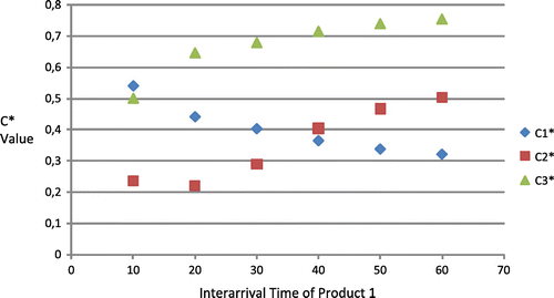
Figure 10. C^* values of products 1, 2 and 3 against different values of mean inter-arrival time of product 2.

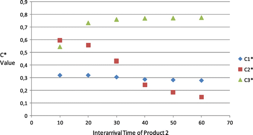
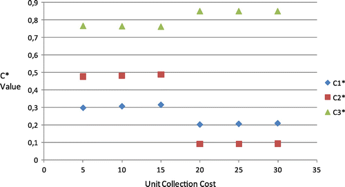
Figure 11 presents a graph of C* values of Products 1, 2 and 3 against six different values of unit collection cost (UCC). The increase in UCC increases the C* value of Product 3, while the C* values of Product 1 and 2 decrease. For all UCC values, the best alternative is Product 3. While the second best alternative is Product 2 for UCC values of 5, 10 and 15, Product 1 outperforms Product 2 for UCC values of 20, 25 and 30.

Figure 11. C^* values of products 1, 2 and 3 against different values of unit collection cost.

6. Conclusions and future research

In this study, used product selection problem faced by 3PRLPs was studied by proposing a four-stage methodology. In the first stage, quantitative and qualitative criteria to be used in the selection process were determined. The weights of the criteria were calculated using fuzzy AHP in the second stage. The third stage involves the calculation of the values of the quantitative criteria using the simulation models constructed for each used product alternative. The ranking of alternative used products were obtained by employing TOPSIS in the fourth stage. A sensitivity analysis was also carried out in order to determine the impact of product arrival rate and unit collection cost on the ranking of used products. Possible managerial insights that can be gained from the proposed approach are as follows:

•	Use of simulation enables decision makers to estimate the value of quantitative criteria by considering the stochastic issues involved in used product evaluation process.
•	Use of Fuzzy AHP and TOPSIS enables decision-makers to include multiple criteria in used product evaluation process.
•	The proposed methodology can be used to evaluate different product structures.
•	When the inter-arrival time of a product decreases its C* value increases. This can be mainly attributed to the fact that higher arrival rate increases the total revenue obtained from the product.

Another problem frequently faced by 3PRLPs is design of a cost-effective reverse logistics network. The papers in the current literature solve this problem by assuming that the types of used products to be collected by the 3PRLP are pre-determined. However, reverse logistic network design will be directly affected by the type of used products collected by the 3PRLP. That is why, development of methodologies for the simultaneous optimisation of network design and used product selection decisions will be an interesting future research topic.

Notes on contributor

Mehmet Ali Ilgin is an assistant professor of industrial engineering at Manisa Celal Bayar University. His research interests are in the areas of environmentally conscious manufacturing, product recovery, reverse logistics, spare parts inventory management, multi-criteria decision making and simulation.

Disclosure statement

No potential conflict of interest was reported by the author.

References

- Azadi, Majid, and Reza Farzipoor Saen. 2011. “A New Chance-constrained Data Envelopment Analysis for Selecting Third-party Reverse Logistics Providers in the Existence of Dual-role Factors.” Expert Systems with Applications 38 (10): 12231–12236. doi:10.1016/j.eswa.2011.04.001.
- Banks, J., J. S. Carson, B. L. Nelson, and D. M. Nicol. 2001. Discrete-Event System Simulation. Upper Saddle River, NJ: Prentice Hall.
- Barker, Theresa J., and Zelda B. Zabinsky. 2008. “Reverse Logistics Network Design: A Conceptual Framework for Decision Making.” International Journal of Sustainable Engineering 1 (4): 250–260. doi:10.1080/19397030802591196.
- Buckley, J. J. 1985. “Ranking Alternatives Using Fuzzy Numbers.” Fuzzy Sets and Systems 15 (1): 21–31. doi:10.1016/0165-0114(85)90013-2.
- Chan, F. T. S., H. K. Chan, and M. H. Chan. 2003. “An Integrated Fuzzy Decision Support System for Multicriterion Decision-making Problems.” Proceedings of the Institution of Mechanical Engineers, Part B: Journal of Engineering Manufacture 217 (1): 11–27.10.1243/095440503762502251
- Chang, Da-Yong. 1996. “Applications of the Extent Analysis Method on Fuzzy AHP.” European Journal of Operational Research 95 (3): 649–655. doi:10.1016/0377-2217(95)00300-2.
- Efendigil, T., Semih Önüt, and Elif Kongar. 2008. “A Holistic Approach for Selecting a Third-party Reverse Logistics Provider in the Presence of Vagueness.” Computers & Industrial Engineering 54 (2): 269–287. doi:10.1016/j.cie.2007.07.009.
- Govindan, Kannan, Joseph Sarkis, and Murugesan Palaniappan. 2013. “An Analytic Network Process-based Multicriteria Decision Making Model for a Reverse Supply Chain.” The International Journal of Advanced Manufacturing Technology 68 (1–4): 863–880. doi:10.1007/s00170-013-4949-2.
- Govindan, Kannan, Hamed Soleimani, and Devika Kannan. 2015. “Reverse Logistics and Closed-loop Supply Chain: A Comprehensive Review to Explore the Future.” European Journal of Operational Research 240 (3): 603–626. doi:10.1016/j.ejor.2014.07.012.
- Hwang, C. L., and K. S. Yoon. 1981. Multiple Attribute Decision Making: Methods and Applications. Berlin: Springer.10.1007/978-3-642-48318-9
- Ilgin, M. A., and S. M. Gupta. 2012. Remanufacturing Modeling and Analysis. Boca Raton, FL: CRC Press.10.1201/b11778
- Ilgin, Mehmet Ali, and Surendra M. Gupta. 2013. “Reverse Logistics.” In Reverse Supply Chains, edited by S. M. Gupta, 1–60. Boca Raton, FL: CRC Press.10.1201/b13749
- Ilgin, Mehmet Ali, and Surendra M. Gupta. 2010. “Environmentally Conscious Manufacturing and Product Recovery (ECMPRO): A Review of the State of the Art.” Journal of Environmental Management 91 (3): 563–591.10.1016/j.jenvman.2009.09.037
- Ilgin, Mehmet Ali, Surendra M. Gupta, and Olga Battaïa. 2015. “Use of MCDM Techniques in Environmentally Conscious Manufacturing and Product Recovery: State of the art.” Journal of Manufacturing Systems 37 (3): 746–758. doi:10.1016/j.jmsy.2015.04.010.
- Kannan, Govindan, Shaligram Pokharel, and P. Sasi Kumar. 2009. “A Hybrid Approach Using ISM and Fuzzy TOPSIS for the Selection of Reverse Logistics Provider.” Resources, Conservation and Recycling 54 (1): 28–36. doi:10.1016/j.resconrec.2009.06.004.
- Kelton, D. W., R. P. Sadowski, and D. A. Sadowski. 2007. Simulation with Arena. 4th ed. New York, NY: McGraw-Hill.
- Ko, Hyun Jeung, and Gerald W. Evans. 2007. “A Genetic Algorithm-based Heuristic for the Dynamic Integrated Forward/Reverse Logistics Network for 3PLs.” Computers & Operations Research 34 (2): 346–366. doi:10.1016/j.cor.2005.03.004.
- Law, A. M. 2007. Simulation Modelling and Analysis. 4th ed. New York, NY: McGraw Hill.
- Lee, Der-Horng, Wen Bian, and Meng Dong. 2007a. “Multiobjective Model and Solution Method for Integrated Forward and Reverse Logistics Network Design for Third-Party Logistics Providers.” Transportation Research Record: Journal of the Transportation Research Board 2032: 43–52.10.3141/2032-06
- Lee, Der-Horng, Wen Bian, and Meng Dong. 2007b. “Multiproduct Distribution Network Design of Third-Party Logistics Providers with Reverse Logistics Operations.” Transportation Research Record: Journal of the Transportation Research Board 2008: 26–33.10.3141/2008-04
- Meade, Laura, and Joseph Sarkis. 2002. “A Conceptual Model for Selecting and Evaluating Third-party Reverse Logistics Providers.” Supply Chain Management: An International Journal 7 (5): 283–295.10.1108/13598540210447728
- Min, Hokey, and Hyun-Jeung Ko. 2008. “The Dynamic Design of a Reverse Logistics Network from the Perspective of Third-party Logistics Service Providers.” International Journal of Production Economics 113 (1): 176–192.10.1016/j.ijpe.2007.01.017
- Nikolaidis, Yiannis. 2009. “A Modelling Framework for the Acquisition and Remanufacturing of Used Products.” International Journal of Sustainable Engineering 2 (3): 154–170. doi:10.1080/19397030902738952.
- Pochampally, Kishore K., and Surendra M. Gupta. 2008. “A Multiphase Fuzzy Logic Approach to Strategic Planning of a Reverse Supply Chain Network.” IEEE Transactions on Electronics Packaging Manufacturing 31 (1): 72–82.10.1109/TEPM.2007.914229
- Rahimifard, S., G. Coates, T. Staikos, C. Edwards, and M. Abu-Bakar. 2009. “Barriers, Drivers and Challenges for Sustainable Product Recovery and Recycling.” International Journal of Sustainable Engineering 2 (2): 80–90. doi:10.1080/19397030903019766.
- Saaty, T. L. 1980. The Analytic Hierarchy Process. New York, NY: McGraw-Hill.
- Saen, R. F. 2010. “A New Model for Selecting Third-party Reverse Logistics Providers in the Presence of Multiple Dual-role Factors.” The International Journal of Advanced Manufacturing Technology 46 (1–4): 405–410. doi:10.1007/s00170-009-2092-x.
- Saen, R. F. 2011. “A Decision Model for Selecting Third-party Reverse Logistics Providers in the Presence of Both Dual-role Factors and Imprecise Data.” Asia-Pacific Journal of Operational Research 28 (2): 239–254. doi:10.1142/S0217595911003156.
- Sasikumar, P., and G. Kannan. 2008a. “Issues in Reverse Supply Chains, Part I: End-of-life Product Recovery and Inventory Management—An Overview.” International Journal of Sustainable Engineering 1 (3): 154–172. doi:10.1080/19397030802433860.
- Sasikumar, P., and G. Kannan. 2008b. “Issues in Reverse Supply Chains, Part II: Reverse Distribution Issues—An Overview.” International Journal of Sustainable Engineering 1 (4): 234–249. doi:10.1080/19397030802509974.
- Sasikumar, P., and G. Kannan. 2009. “Issues in Reverse Supply Chain, Part III: Classification and Simple Analysis.” International Journal of Sustainable Engineering 2 (1): 2–27. doi:10.1080/19397030802673374.
- Shaharudin, Mohd Rizaimy, Suhaiza Zailani, and Mahazir Ismail. 2014. “Third Party Logistics Orchestrator Role in Reverse Logistics and Closed-loop Supply Chains.” International Journal of Logistics Systems and Management 18 (2): 200–215.10.1504/IJLSM.2014.062326
- Suyabatmaz, Ali Cetin, F. Altekin, and Guvenc Şahin. 2014. “Hybrid Simulation-Analytical Modeling Approaches for the Reverse Logistics Network Design of a Third-party Logistics Provider.” Computers & Industrial Engineering 70: 74–89. doi:10.1016/j.cie.2014.01.004.
- Triantaphyllou, Evangelos, and Chi-Tun Lin. 1996. “Development and Evaluation of Five Fuzzy Multiattribute Decision-making Methods.” International Journal of Approximate Reasoning 14 (4): 281–310.10.1016/0888-613X(95)00119-2
- Tsaur, S., T. Chang, and C. Yen. 2002. “The Evaluation of Airline Service Quality by Fuzzy MCDM.” Tourism Management 23: 107–115.10.1016/S0261-5177(01)00050-4
- van Laarhoven, P. J. M., and W. Pedrycz. 1983. “A Fuzzy Extension of Saaty’s Prizority Theory.” Fuzzy Sets and Systems 11 (1–3): 199–227. doi:10.1016/S0165-0114(83)80082-7.
- Zadeh, L. A. 1965. “Fuzzy sets.” Information and Control 8: 338–353.10.1016/S0019-9958(65)90241-X