A multi-path routing-inventory problem for a closed-loop supply chain considering the heterogeneous fleet of vehicles

ABSTRACT

In this paper, the inventory-routing problem is studied for a closed-loop supply chain. This closed-loop supply chain considers suppliers, manufacturers, whole-sellers, and disposal centers. To formulate this problem, a mixed integer linear programming model is proposed. This mathematical model minimizes the total costs of the supply chain, including the fixed and variable costs of vehicles, and holding inventory costs of final products and scraps. The proposed model considers the road roughness degree, multi-path setting and the heterogeneous fleet of vehicles, which increases its flexibility and the quality of solutions. Then, two symmetry-breaking constraints are proposed to reduce the complexity of the mathematical model. In order to evaluate the integrity of the proposed model, 20 instances of different sizes are randomly generated and solved. Finally, a comprehensive sensitivity analysis is conducted with respect to five key features of the problem, such as the impact of the symmetry-breaking constraints on the CPU time, multi-path setting, fixed cost of vehicles, heterogeneous fleet of vehicles, and lost sales. The results indicate that the consideration of multi-path setting and the heterogeneous fleet of vehicles improves the quality of solutions significantly.

KEYWORDS:

• Closed-loop supply chain
• inventory control
• vehicle routing problem
• heterogeneous fleet of vehicle
• multi-path

1. Introduction

Nowadays, the world is struggling with many catastrophes, including human-being diseases and natural disasters. Global warming, as one of the most important natural disasters, is gradually increasing due to the emission of the environmental contaminants. Such environmental pollutions also endanger many species (Du et al. 2015). In the real world, scraps of a few industries (such as bakery) do not contain toxic wastes, and disposing of them directly to the environment would not damage it. On the other hand, scraps of many other industries (such as battery) contain hazardous wastes that direct disposal of them to the environment might severely damage it. The classic Supply Chain (SC) design, which is known as forward SC, does not take any responsibility for scraps. Then, this problem has drawn the attention of researchers and led to the creation of reverse SC notion. The reverse SC design mainly concerns about the ways that SCs consider to recycle scraps returned by customers.

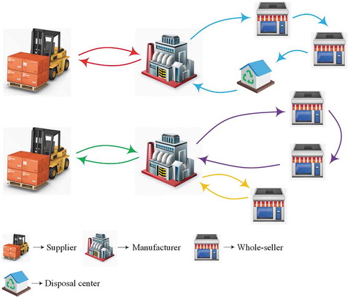
The environmental awareness of people forced governments to enact some regulations and provide incentive schemes for production companies to take care of scraps (Alimoradi, Yussuf, and Zulkifli 2011). Therefore, organizations mostly include disposal centers as a separate echelon in SC design besides the forward flow. In other words, they have started to consider both forward and reverse flows and created a new concept called the Closed-Loop Supply Chain (CLSC) (Govindan and Soleimani 2017). Beyond these reasons, reducing the total costs of organizations is another incentive to change the traditional SCs with new designs (Alimoradi et al. 2015). In the CLSC, the focus is on taking the responsibility of returned products from consumers and reusing the entire of or a part of them (Jena and Sarmah 2016). Consumers may return products for different reasons during and after the products’ life cycle. Commercial returns may occur in at most a 90-day period after procurement. In addition, other types of returns, like repair, end-of-use and end-of-life returns, may even occur decades after purchase (Guide and Wassenhove 2006). As the CLSC design has attracted the attention of many researchers, many recently published papers in the literature covered this concept, e.g. Tosarkani and Amin (2018), Shankar, Bhattacharyya, and Choudhary (2018), Bazan, Jaber, and Zanoni (2017), Üster and Hwang (2017), Mawandiya, Jha, and Thakkar (2016) and Kuo (2011). For the same reasoning, we have also been motivated to study a four-echelon CLSC design. This CLSC design includes suppliers, manufacturers, whole-sellers, and disposal centers. For more clarification, Figure 1 illustrates a typical schema for the CLSC design investigated in this paper.

Figure 1. A typical schema for the problem considered in this study.

Considering the fact that there would be more than one path between any two nodes, these paths may vary in terms of distance and road roughness degree. Consequently, we have considered the multi-path setting. It will increase the flexibility of SC design, and increase the efficiency of the routing problem. For instance, path $\mathit{A}$ between a pair of nodes might be shorter than path $\mathit{B}$ between the same nodes, but it might be worse than path $\mathit{B}$ regarding the road roughness degree. Although the former path is shorter and decreases the travel time, it might increase the fuel cost significantly; thus, we would prefer the latter one. According to Gentle (1997), the higher road roughness degree increases the amount of fuel consumed by a vehicle. Fahimnia et al. (2013a) proposed a model for a forward SC design considering the impact of road roughness degree on fuel consumption and discussed its importance. However, they did not consider the multi-path setting in their study, which is also essential, based on the example provided above.

In real-world problems, organizations generally own a limited number of vehicles, which would vary in terms of capacity and fuel consumption rate. For example, larger trucks are used to transport raw materials from suppliers to manufacturers; whereas, smaller vehicles are used to transport products from manufacturers to whole-sellers. This happens since demands of whole-sellers are mostly fewer than manufacturers. Many of the previous investigations neglected limited numbers of vehicles, the limited capacity of vehicles and the heterogeneous fleet of vehicles, e.g. Tosarkani and Amin (2018), Kaya and Urek (2016), and Kannan et al. (2012). Some of the previous studies only addressed the limited capacity vehicles, e.g. Talaei et al. (2016), and Zakeri et al. (2015). Finally, some other merely studied the heterogeneous fleet of vehicles, e.g. Rahmani and Mahmoodian (2017), and Fahimnia et al. (2015). To the best knowledge of authors, there is no paper in the literature, which has been studied these three features at the same time. For this purpose, we have considered all of them in this paper.

In contrast to many previous investigations, we have studied a multi-period problem. Under this condition, manufactures and whole-sellers are capable of storing raw materials and final products, respectively. As the same as multi-path setting, holding inventory adds flexibility to the modeling and increases the quality of solutions. In some cases, unnecessary travel could be prevented by holding a small number of inventories. Note that holding inventory is not applicable for some industries depending on the essence of raw materials or final products. Many studies have ignored it, e.g. Üster and Hwang (2017), and Talaei et al. (2016). However, some other studies have considered it, e.g. Tosarkani and Amin (2018), and Kaya and Urek (2016). In this study, we have also assumed that manufacturers and whole-sellers are capable of holding inventories.

The remainder of this paper is organized as follows. Following a comprehensive review of the literature in Section 2, the problem is described in Section 3. This section also proposes the mathematical model of this problem. Section 4 presents a numerical example and a comprehensive sensitivity analysis. Finally, Section 5 provides the conclusions, remarks and future research directions.

2. Literature review

Focusing on SC Management (SCM) has been rapidly increasing since the last decade. Global warming and air pollution could be the principal reasons for this as well as the importance of cutting cost. This paper addresses several studies concentrating on SCM. We begin this section by reviewing forward or reverse SCs. Afterward, we review several CLSCs.

Kannan et al. (2012) studied a reverse logistics network with sensitivity to carbon emission; the objective of this study is to minimize the cost and the carbon emission resulting from the vehicles of the logistic system. Aalaei and Davoudpour (2017) investigated a forward SC under uncertainty of demand; accordingly, a robust optimization was developed. The proposed model aims to minimize costs of transportation, holding inventory, production, and labor. Rahmani and Mahoodian (2017) took into account the strategic and operational planning phase in a forward supply chain. They studied the heterogeneous fleet of vehicles and considered two types of vehicles. In order to reduce the distance traveled by vehicles, they concluded that the optimization of the number of distribution centers is necessary. Keshari et al. (2017) considered the heterogeneous fleet of vehicles in their SC design. In addition, Ordering-up to policy has been utilized to alleviate the bullwhip effect and satisfy customers demand while the total cost of SC is minimized. Fahimnia et al. (2015) developed a forward SC model by focusing on the carbon tax. They also assumed other features such as holding inventory, the heterogeneous fleet of vehicles, and multi-period setting. They applied the model to a real case study in Australia and indicated that the model reduces carbon emission significantly. Rakke et al. (2011) investigated a worldwide maritime delivery problem for one of the largest producers of Liquefied Natural Gas (LNG) in the world. They aimed to design an annual delivery plan in order to simultaneously fulfill long-term contracts at an optimal cost and maximize the revenue of selling LNG in spot markets. A mix integer programing model is presented for the problem. Then, a rolling horizon heuristic is developed to deal with the complexity of the model. Stålhane et al. (2012) studied the identical problem. However, they developed a construction and improvement heuristic method, and showed that the proposed solution approach is more efficient regarding CPU time as compared to that of Rakke et al. (2011). Archetti, Christiansen, and Grazia Speranza (2018) merged pick-up and delivery vehicle routing and inventory management problems. They assumed that a single vehicle obtains a commodity from several origins and distributes it among multiple demand points. They developed a branch-and-cut method to solve the proposed mathematical model. They also concluded that the integrated model cuts cost up to 35% compared to non-integrated one. These papers, however, differs from ours. First, all papers mentioned above studied forward or reverse SCs; while we investigated a CLSC design. Second, we considered other features such as road roughness degree and multi-path setting in the paper under consideration.

Savaskan, Bhattacharya, and Wassenhove (2004) compared three different policies of collecting scraps from customers in a CLSC system. The first policy is to hire a third-party company in order to gather scraps and return them to a single manufacturer. In the second policy, the manufacturer collects scraps directly from customers. The last policy comprises providing incentives for the existing retailers to collect scraps instead of the manufacturer. They showed that the CLSC could be designed in a way to increase profit and market demand as well as scraps return rate; the last policy is suggested to accomplish these goals better than the two others do. Kaya and Urek (2016) studied a CLSC concentrating on holding inventory, pricing, and locating issues. They developed a mixed integer linear programming for the problem. Then, they proposed three metaheuristic algorithms to solve the problem and showed which one performs better. Bazan, Jaber, and Zanoni (2017) compared classic and vendor managed inventory SC designs for a two-echelon CLSC with a single player in each echelon. The vendor managed inventory SC mechanism is showed to be more economical for a broad range of annual investment to manufacturing rate. However, they argued that the classic SC designs are more environmentally responsible. Tao et al. (2015) introduced a multi-period dynamic CLSC design. In this dynamic CLSC design, they specified several planning horizons; they assumed that all input data are stable in each planning horizons but different across various planning horizons. Zakeri et al. (2015) consider the limited capacity of vehicles in a multi-period CLSC design. They assumed two different scenarios reflecting two environmental regularities. Then, a real case study is used to analyze the output of the proposed mathematical model in these scenarios. Mohammed et al. (2017) proposed an optimization model for a multi-period CLSC design. The limited capacity of vehicles is also considered in this study. Nevertheless, the primary concern of the study is about carbon emission. Fahimnia et al. (2013b) considered the heterogeneous fleet of vehicles in the CLSC. They used a case study in Australia to analyze the performance of the proposed model focusing on the carbon tax.

To better indicate the novelty of our paper, we have identified four studies in the literature that are more similar to ours than all the other papers mentioned above. Soysal et al. (2015) studied a CLSC design for the food industry. In addition to the limited capacity of vehicles, they took into account the finite number of vehicles. This investigation aims to account for perishability, fuel consumption, and demand uncertainty. They showed that the consideration of perishability and fuel consumption makes the model more useful. Iassinovskaia, Limbourg, and Riane (2017) considered a homogeneous vehicle fleet for a pick-up and delivery inventory routing problem with time window. A mix-integer linear programing model is developed for the problem; then, they proposed a cluster first-route second metaheuristic to deal with large instances. Zhang, Alshraideh, and Diabat (2018) took carbon emission regulations into account in a reverse SC under demand uncertainty. They considered the limited heterogeneous vehicles for transportation. A mathematical model is proposed for this problem. The result of simulation illustrated that carbon price as the most significant parameter of the model. Rahimi, Baboli, and Rekik (2017) studied a CLSC problem with heterogeneous vehicle fleet. The study aimed to simultaneously minimize cost, curb air pollution, and minimize delay and backorder quantity by determining an optimal service level. They concluded that choosing the service level when logistic components are also considered is beneficial for the entire system. Considering what was mentioned earlier, our paper differs from all these four papers respecting different features. First, with this investigation studying the multi-path setting, none of these papers has studied this feature. Second, our paper takes into account the impact of the road roughness on the fuel consumption of vehicles; whereas none of these papers has considered this feature. As explained in Section 1, considering the multi-path setting and the road roughness degree simultaneously could increase the flexibility of the model and quality of solutions. Moreover, none of these papers has studied the limited numbers of vehicles, the limited capacity of vehicles and the heterogeneous fleet of vehicles for CLSC, simultaneously. This set of features is essential to simulate the real-world setting.

To better illustrate the novelty of our investigation, we have summarized the features of several recent studies in Table 1 and compared with our paper. Considering this table, the main contributions of this paper are as follows:

• This paper studies the multi-path setting and road roughness degree.

• This paper considers the limited numbers of vehicles, the limited capacity of vehicles and the heterogeneous fleet of vehicles for CLSC, simultaneously.

Table 1. Comparison between the features of several recent studies and the current study.

Author(s)	Type of SC	Road roughness degree	Multi- path	Holding cost	Limited number of vehicles	Capacity of vehicles	Heterogeneous fleet of vehicles	Multi- period
Tosarkani and Amin (2018)	CLSC	-	-	†	-	-	-	†
Kaya and Urek (2016)	CLSC	-	-	†	-	-	-	-
Bazan, Jaber, and Zanoni (2017)	CLSC	-	-	†	-	-	-	-
Kannan et al. (2012)	Reverse SC	-	-	-	-	-	-	-
Shankar, Bhattacharyya, and Choudhary (2018)	CLSC	-	-	†	-	-	-	†
Üster and Hwang (2017)	CLSC	-	-	-	-	-	-	-
Fahimnia et al. (2013a)	Forward SC	†	-	-	-	-	-	†
Fahimnia et al. (2015)	Forward SC	-	-	†	-	-	†	†
Rahmani and Mahoodian (2017)	Forward SC	-	-	-	-	-	†	-
Talaei et al. (2016)	CLSC	-	-	-	-	†	-	-
Fahimnia et al. (2013b)	CLSC	-	-	†	-	-	†	†
Tao et al. (2015)	CLSC	-	-	†	-	-	-	†
Zakeri et al. (2015)	CLSC	-	-	†	-	†	-	†
Aalaei and Davoudpour (2017)	Forward SC	-	-	†	-	-	-	-
Soysal et al. (2015)	CLSC	-	-	†	†	†	-	†
Soysal (2016)	CLSC	-	-	†	†	†	-	†
Choudhary et al. (2015)	CLSC	-	-	-	-	†	-	-
Mohammed et al. (2017)	CLSC	-	-	†	-	†	-	†
Keshari et al. (2017)	Forward SC	-	-	†	-	-	†	-
Alhaj, Svetinovic, and Diabat (2016)	Forward SC	-	-	†	-	-	-	-
Rahimi, Baboli, and Rekik (2017)	CLSC	-	-	†	-	†	†	†
Iassinovskaia, Limbourg, and Riane (2017)	CLSC	-	-	†	†	†	-	†
Zhang, Alshraideh, and Diabat (2018)	Reverse SC	-	-	†	†	†	†	†
Archetti, Christiansen, and Grazia Speranza (2018)	Forward SC	-	-	†	†	†	-	†
Current study	CLSC	†	†	†	†	†	†	†

3. Mathematical formulation

3.1. Problem description

As stated, this paper intends to study a four-echelon SC design. This SC includes a number of suppliers, manufacturers, whole-sellers and disposal centers. To begin with, let us look at how the raw materials, final products, and scraps flow in the system. Manufacturers acquire the raw materials from both suppliers and disposal centers. Whole-sellers also obtain the final products from manufacturers and send scraps to disposal centers. Recycling a portion of scraps, disposal centers make raw materials out of them, then, send them back to manufacturers (clarified in Figure 1). Since this paper studies the multi-path setting, there would be more than one path between any of two nodes. The distance of each of these paths is already determined. Due to the fact that vehicles travel with a fixed mean speed, therefore, the time required to travel between nodes is also determined for each path.

In this paper, we have assumed that two types of vehicles deliver items through this CLSC design. The first type of vehicles transports raw materials from suppliers to manufacturers, and the second type of vehicles transports items (i.e. final products, scraps, and raw materials) among manufacturers, whole-sellers and disposal centers. These types are different in capacity, fixed and variable costs. Moreover, vehicles might give service to more than one whole-seller after leaving manufacturers. The demand for whole-sellers is assumed to be already determined. Besides, all demands need to be satisfied. In other words, the backorder is not allowed in the system. Whole-sellers are capable of holding final products to answer the demands of next periods; they can also hold scraps and send them to disposal centers in later periods. However, holding final products or scraps imposes extra costs to the system.

The objective of this problem is to minimize the various costs of this CLSC design. These costs include the fixed cost of using vehicles, variable costs (costs of using vehicles and hiring drivers), and holding inventory costs of final products and scraps.

The assumptions considered in this study are as follows:

• Number, location, and capacity of suppliers, manufacturers, and whole-sellers are already known.

• There might be more than one path between two specific nodes.

• The distance between two nodes and the time required to travel them are already determined.

• Demands of whole-sellers for all periods are already known.

• Backordering is not allowed.

• A fraction of scraps will be disposed at disposal centers; the rest of them will be recycled and sent back to the manufacturers as raw materials.

Considering all the points mentioned earlier, we have proposed a mathematical model in the following sub-section.

3.2. The proposed model

In order to formulate the proposed model, we first need to introduce the notations as follows.

● Indices:

$i$, $j$	=	Index of nodes
$t$	=	Index of periods
$k$	=	Index of the types of vehicles
$p$	=	Index of paths

● Sets:

$\mathcal{S}$	=	Set of suppliers
$\mathcal{M}$	=	Set of manufacturers
$\mathcal{R}$	=	Set of whole-sellers
$\mathcal{D}$	=	Set of disposal centers
$\mathcal{A}$	=	Set of all nodes (including suppliers, manufacturers, whole-sellers and disposal centers)
$\mathcal{T}$	=	Sets of periods
E	=	Set of vehicles that travel between suppliers, and manufacturers (first type of vehicles)
$\mathcal{G}$	=	Set of vehicles that travel between manufacturers, whole-sellers, and disposal centers (second type of vehicles)
$\mathcal{F}$	=	Set of all vehicles (including the first and second types of vehicles)
$\mathcal{P}$	=	Sets of paths

● Parameters:

$D_{ijp}$	=	The distance between node $i$ and node $j$ using path $p$ (based on kilometer)
$W_{ijp}$	=	The time required to travel from node $i$ to node $j$ using path $p$ (based on hour)
$C_{1k}$	=	The fixed cost of using vehicle type $k$
$C_{2k}$	=	The variable cost of using vehicle type $k$ (per kilometer)
$C_{3k}$	=	Cost of hiring driver for vehicle type $k$ (per hour)
$P_i$	=	The production capacity of node $i$ (where $i\in \mathcal{S}\cup \mathcal{M}$)
$C{S}_i$	=	The capacity of node $i$ to hold scraps (where $i\in \mathcal{R}$)
$C{F}_i$	=	The capacity of node $i$ to hold final products (where $i\in \mathcal{R}$)
$H_{1t}$	=	Holding cost of final products at period $t$ (per each unit)
$H_{2t}$	=	Holding cost of scraps at period $t$ (per each unit)
$O_{it}$	=	The demand of node $i$ at period $t$ (where $i\in \mathcal{R}$)
$V_{it}$	=	Number of scraps received in node $i$ at period $t$
$DP$	=	Percentage of scraps which would be disposed at disposal centers
$Q_1$	=	The capacity of the first type of vehicles that travel between suppliers and manufacturers
$Q_2$	=	The capacity of the second type of vehicles that travel between manufacturers, whole-sellers and disposal centers
$L_{1ik}$	=	If vehicle $k$ belongs to node $i$, 1; otherwise, 0 (where $i\in \mathcal{S}$ and $k\in$E)
$L_{2ik}$	=	If vehicle $k$ belongs to node $i$, 1; otherwise, 0 (where $i\in \mathcal{M}$ and $k\in \mathcal{G}$)
${\mu }_{ijp}$	=	Road roughness degree between nodes $i$ and $j$ using path $p$
${\omega }_{ijp}$	=	Variable cost adjustment coefficient between nodes $i$ and $j$ using path $p$

● Decision variables:

$x_{ijkpt}$	=	If vehicle $k$ moves from node $i$ toward node $j$ at period $t$ using path $p$, 1; otherwise, 0.
$y_{ijkpt}$	=	Load of vehicle $k$ moving from node $i$ toward node $j$ at period $t$ using path $p$ (final products)
$z_{ijkpt}$	=	Load of vehicle $k$ moving from node $i$ toward node $j$ at period $t$ using path $p$ (scraps)
$h_{1it}$	=	The final products held in node $i$ at period $t$ (where $i\in \mathcal{R}$)
$h_{2it}$	=	The scraps held in node $i$ at period $t$ (where $i\in \mathcal{R}$)
$u_{ikt}$	=	A positive auxiliary variable for the elimination of sub-tours

Based on these preliminary definitions, the intended mathematical model is formulated as follows:

(1) $\begin{array}{rl}& Minf=\sum _{i\in \mathcal{S}\cup \mathcal{M}}\sum _{j\in \mathcal{M}\cup \mathcal{R}\cup \mathcal{D}}\sum _{k\in \mathcal{F}}\sum _{p\in \mathcal{P}}\sum _{t\in \mathcal{T}}{x}_{ijkpt}{C}_{1k}\\ & +\sum _{i,j\in \mathcal{A}}\sum _{k\in \mathcal{F}}\sum _{p\in \mathcal{P}}\sum _{t\in \mathcal{T}}(x_{ijkpt}{D}_{ijp}{\omega }_{ijp}{C}_{2k}+x_{ijkpt}{W}_{ijp}{C}_{3k})\\ & +\sum _{i\in \mathcal{R}}\sum _{t\in \mathcal{T}}{h}_{1it}{H}_{1t}+\sum _{i\in \mathcal{R}}\sum _{t\in \mathcal{T}}{h}_{2it}{H}_{2t}\end{array}$(1)

The objective function minimizes total costs. To be more precise, the first term aims to minimize the fixed of using vehicles. The second term minimizes the variable costs, including costs of fuel, depreciation, and hiring of drivers. Finally, the third and fourth terms minimize the holding inventory costs of final products and scraps, respectively. This objective function is limited to the following constraints:

(2) $\sum _{j\in \mathcal{M}\cup \mathcal{R}}\sum _{k\in \mathcal{F}}\sum _{p\in \mathcal{P}}{y}_{ijkpt}\le P_i\mathrm{\forall }i\in \mathcal{S}\cup \mathcal{M};t\in \mathcal{T}$(2)

${\sum }_{p\in \mathcal{P}}{y}_{ijkpt}\le Q_1{\sum }_{p\in \mathcal{P}}{x}_{ijkpt}\mathrm{\forall }i\in \mathcal{S};j\in \mathcal{M};k\in$E$;t\in \mathcal{T}(3)$

(4) ${\sum }_{p\in \mathcal{P}}{y}_{ijkpt}\le Q_2{\sum }_{p\in \mathcal{P}}{x}_{ijkpt}\mathrm{\forall }i\in \mathcal{M};j\in \mathcal{R};k\in \mathcal{G};t\in \mathcal{T}$(4)

(5) ${\sum }_{p\in \mathcal{P}}{y}_{ijkpt}\le Q_2{\sum }_{p\in \mathcal{P}}{x}_{ijkpt}\mathrm{\forall }i\in \mathcal{D};j\in \mathcal{M};k\in \mathcal{G};t\in \mathcal{T}$(5)

(6) ${\sum }_{p\in \mathcal{P}}{z}_{ijkpt}\le Q_2{\sum }_{p\in \mathcal{P}}{x}_{ijkpt}\mathrm{\forall }i\in \mathcal{R};j\in \mathcal{D};k\in \mathcal{G};t\in \mathcal{T}$(6)

(7) ${\sum }_{p\in \mathcal{P}}{y}_{ijkpt}+{\sum }_{p\in \mathcal{P}}{z}_{ijkpt}\le Q_2{\sum }_{p\in \mathcal{P}}{x}_{ijkpt}\mathrm{\forall }i,j\in \mathcal{R};k\in \mathcal{G};t\in \mathcal{T}$(7)

Constraint (2) ensures that each of suppliers and manufacturers could not supply raw materials or final products more than their capacity. Constraints (3–7) guarantee that vehicles do not transport items (raw materials, final products, and scraps) more than their capacity. In other words, the total load of a vehicle has to be less than or equal to its capacity. Constraint (3) refers to the limited capacity of the first type vehicles, while Constraints (4–7) address the limited capacity of the second type of vehicles.

(8) $\begin{array}{rl}& {\sum }_{i\in \mathcal{R}}{\sum }_{k\in \mathcal{G}}{\sum }_{p\in \mathcal{P}}{y}_{jikpt}={\sum }_{i\in S}{\sum }_{k\in \mathcal{E}}{\sum }_{p\in \mathcal{P}}{y}_{ijkpt}\\ & +{\sum }_{i\in \mathcal{D}}{\sum }_{k\in \mathcal{G}}{\sum }_{p\in \mathcal{P}}\\ & y_{ijkp\left(t-1\right)}\mathrm{\forall }j\in \mathcal{M};t\in \mathcal{T}\end{array}$(8)

(9) $\begin{array}{rl}& {\sum }_{i\in \mathcal{R}}{\sum }_{k\in \mathcal{G}}{\sum }_{p\in \mathcal{P}}{z}_{ijkpt}-DP{\sum }_{i\in \mathcal{R}}{\sum }_{k\in \mathcal{G}}\\ & {\sum }_{p\in \mathcal{P}}{z}_{ijkpt}={\sum }_{i\in \mathcal{M}}{\sum }_{k\in \mathcal{G}}{\sum }_{p\in \mathcal{P}}{y}_{jikpt}\\ & \mathrm{\forall }j\in \mathcal{D};t\in \mathcal{T}\end{array}$(9)

Constraint (8) assures that the final products sent to whole-sellers from each manufacturer are equal to the raw materials sent to the same manufacturer from suppliers and disposal centers. Constraint (9) also guarantees that a faction of scraps (i.e. $DP$) is disposed at disposal centers, and the rest of them are sent back to manufacturers as raw materials.

(10) $\begin{array}{l}{O}_{it}={\sum }_{j\in ℳ}{\sum }_{k\in \mathcal{G}}{\sum }_{p\in }{y}_{jikpt}+{\sum }_{j\in ℛ}{\sum }_{k\in \mathcal{G}}\\ {\displaystyle \sum _{p\in }{y}_{jikpt}}-{\sum }_{j\in ℛ}{\sum }_{k\in \mathcal{G}}{\sum }_{p\in }{y}_{ijkpt}\\ -h_{1it}+h_{1i\left(t-1\right)}\forall i\in ℛ;t\in \mathcal{T}\end{array}$(10)

(11) $h_{1it}\le C{F}_i\mathrm{\forall }i\in \mathcal{R};t\in \mathcal{T}$(11)

Constraint (10) ensures that the demand of whole-sellers has to be satisfied. In fact, this constraint creates a trade-off between the input and output flows of final products within whole-sellers (i.e. the final products coming into whole-sellers from manufacturers and other whole-sellers, and the final products sent from them to satisfy the demand of other whole-sellers), and the final products held within them at the previous and current periods. Constraint (11) also ensures that the final products held within whole-sellers have to be less than or equal to their capacity.

(12) $\begin{array}{l}{\sum }_{j\in ℛ}{\sum }_{k\in \mathcal{G}}{\sum }_{p\in }{z}_{ijkpt}+{\sum }_{j\in \mathcal{D}}{\sum }_{k\in \mathcal{G}}\\ {\sum }_{p\in }{z}_{ijkpt}={\sum }_{j\in ℛ}{\sum }_{k\in \mathcal{G}}{\displaystyle \sum _{p\in }{z}_{jikpt}}+V_{it}\\ -h_{2it}+h_{2i\left(t-1\right)}\forall i\in ℛ;t\in \mathcal{T}\end{array}$(12)

(13) $\begin{array}{l}{\displaystyle \sum _{j\in ℛ}{\displaystyle \sum _{p\in }{z}_{ijkpt}}}+{\displaystyle \sum _{j\in \mathcal{D}}{\displaystyle \sum _{p\in }{z}_{ijkpt}}}\ge {\displaystyle \sum _{j\in ℛ}{\displaystyle \sum _{p\in }{z}_{ijkpt}}}\\ \forall i\in ℛ;k\in \mathcal{G};t\in \mathcal{T}\end{array}$(13)

(14) $h_{2it}\le C{S}_i\mathrm{\forall }i\in \mathcal{R};t\in \mathcal{T}$(14)

Like Constraint (10), Constraint (12) creates a trade-off between the input and output flows of scraps within whole-sellers and the number of scraps held in them. Constraint (13) also assures that the number of scraps sent to a whole-seller is less than or equal to the scraps sent from that whole-seller to other whole-sellers and disposal centers. In other words, this constraint forces vehicles to carry all scraps assigned to them within a tour. Constraint (14) ensures that the scraps held in a whole-seller have to be less than or equal to its capacity.

${\sum }_{j\in ℳ}{\displaystyle \sum { }_{p\in }{x}_{ijkpt}}\le 1\forall i\in \mathcal{S};k\in$E$;t\in \mathcal{T}(15)$

(16) ${\sum }_{j\in \mathcal{R}\cup \mathcal{D}}{\sum }_{p\in \mathcal{P}}{x}_{ijkpt}\le 1\mathrm{\forall }i\in \mathcal{M};k\in \mathcal{G};t\in \mathcal{T}$(16)

(17) ${\sum }_{j\in \mathcal{M}\cup \mathcal{R}\cup \mathcal{D}}{\sum }_{p\in \mathcal{P}}{x}_{ijkpt}\le 1\mathrm{\forall }i\in \mathcal{R};k\in \mathcal{G};t\in \mathcal{T}$(17)

(18) ${\sum }_{j\in \mathcal{M}}{\sum }_{p\in \mathcal{P}}{x}_{ijkpt}\le 1\mathrm{\forall }i\in \mathcal{D};k\in \mathcal{G};t\in \mathcal{T}$(18)

Constraint (15) indicates that vehicles of the first type could travel from suppliers to manufacturers. Constraint (16) states that vehicles of the second type could travel from manufacturers to whole-sellers and disposal centers. Constraint (17) also ensures that vehicles of the second type can travel from whole-sellers to manufacturers, other whole-sellers, and disposal centers. Eventually, Constraint (18) indicates that vehicles of the second type can travel from disposal centers to manufacturers.

(19) ${\displaystyle \sum _{j\in ℳ}{\displaystyle \sum _{p\in }{x}_{ijkpt}}}={\displaystyle \sum _{j\in ℳ}{\displaystyle \sum _{p\in }{x}_{jikpt}}}\forall i\in \mathcal{S};k\in E;t\in \mathcal{T}$(19)

(20) ${\displaystyle \sum _{j\in ℛ\cup \mathcal{D}}{\displaystyle \sum _{p\in }{x}_{ijkpt}}}={\displaystyle \sum _{j\in ℛ\cup \mathcal{D}}{\displaystyle \sum _{p\in }{x}_{jikpt}}}\forall i\in ℳ;k\in \mathcal{G};t\in \mathcal{T}$(20)

(21) $\begin{array}{rl}& \sum _{i\in \mathcal{M}}\sum _{p\in \mathcal{P}}{x}_{ijkpt}+\sum _{i\in \mathcal{R}}\sum _{p\in \mathcal{P}}{x}_{ijkpt}=\sum _{i\in \mathcal{M}}\sum _{p\in \mathcal{P}}{x}_{jikpt}+\sum _{i\in \mathcal{R}}\sum _{p\in \mathcal{P}}{x}_{jikpt}\\ & +\sum _{i\in \mathcal{D}}\sum _{p\in \mathcal{P}}{x}_{jikpt}\mathrm{\forall }j\in \mathcal{R};\\ & k\in \mathcal{G};t\in \mathcal{T}\end{array}$(21)

(22) $\begin{array}{rl}& \sum _{i\in \mathcal{M}}\sum _{p\in \mathcal{P}}{x}_{ijkpt}+\sum _{i\in \mathcal{R}}\sum _{p\in \mathcal{P}}{x}_{ijkpt}=\sum _{i\in \mathcal{M}}\sum _{p\in \mathcal{P}}{x}_{jikpt}\\ & \mathrm{\forall }j\in \mathcal{D};k\in \mathcal{G};t\in \mathcal{T}\end{array}$(22)

Constraint (19) assures that if a vehicle of the first type leaves supplier $i$, then, it comes back to the same supplier. Constraint (20) also guarantees that if a vehicle of the second type leaves manufacturer $i$, then, it comes back to the same manufacturer. Constraint (21) guarantees that if a vehicle of the second type travels toward a whole-seller, it leaves the whole-seller toward a manufacturer, or one another whole-seller or a disposal center. Constraint (22) ensures that if a vehicle travels from a manufacturer or a whole-seller to a disposal center, it leaves the disposal center toward a manufacturer.

${\displaystyle \sum _{j\in ℛ\cup \mathcal{D}}{\displaystyle \sum _{p\in }{x}_{ijkpt}}}={\displaystyle \sum _{j\in ℛ\cup \mathcal{D}}{\displaystyle \sum _{p\in }{x}_{jikpt}}}\forall i\in ℳ;k\in \mathcal{G};t\in \mathcal{T}$E$;t\in \mathcal{T}(23)$

(24) ${\displaystyle \sum _{j\in ℛ\cup \mathcal{D}}{\displaystyle \sum _{p\in }{x}_{ijkpt}}}\le L_{2ik}\forall i\in ℳ;k\in \mathcal{G};t\in \mathcal{T}$(24)

Constraints (23 and 24) indicate that the vehicles of the first and second types belong to which of the suppliers and manufacturers, respectively.

(25) $\begin{array}{rl}& u_{ikt}-u_{jkt}+\left|\mathcal{R}\cup \mathcal{D}\right|.x_{ijkpt}\le \left|\mathcal{R}\cup \mathcal{D}\right|-1\\ & \mathrm{\forall }i,j\in \mathcal{R};k\in \mathcal{G};p\in \mathcal{P};t\in \mathcal{T}\end{array}$(25)

Constraint (25) is a sub-tour elimination constraint, where $\left|\mathcal{R}\cup \mathcal{D}\right|$ refers to the cardinality of the union of sets $\mathcal{R}$ and $\mathcal{D}$. For the sake of brevity, we do not provide further details of this constraint here and refer the interested readers to Kara, Laporte, and Bektas (2004).

(26) $x_{ijkpt}\in \left\{0,1\right\}\mathrm{\forall }i,j\in \mathcal{A};k\in \mathcal{F};p\in \mathcal{P};t\in \mathcal{T}$(26)

(27) $\begin{array}{rl}& y_{ijkpt},\hspace{0.17em}{z}_{ijkpt},h_{1it},\hspace{0.17em}{h}_{2it}\ge 0,\hspace{0.17em}integer\mathrm{\forall }i,j\in \mathcal{A};k\in \mathcal{F};\\ & p\in \mathcal{P};t\in \mathcal{T}\end{array}$(27)

(28) $u_{ikt}\ge 0\mathrm{\forall }i\in \mathcal{A};k\in \mathcal{F};t\in \mathcal{T}$(28)

Constraint (26) shows the binary decision variables, Constraint (27) indicates the positive integer decision variables, and Constraints (28) specifies the positive decision variables.

It should be noted that, to approximate the variable cost adjustment coefficient (i.e. ${\omega }_{ijp}$) based on the road roughness degree (i.e. ${\mu }_{ijp}$), we have used the following equation (Sinha and Labi 2007):

(29) ${\omega }_{ijp}=0.001{\left[\left(\frac{{\mu }_{ijp}}{\begin{array}{c}0.0158-80\end{array}}\right)/10\right]}^2-0.018\left[\left(\frac{{\mu }_{ijp}}{\begin{array}{c}0.0158-80\end{array}}\right)/10\right]+0.9991\mathrm{\forall }i\in \mathcal{A};k\in \mathcal{F};t\in \mathcal{T}$(29)

3.3. Symmetry-breaking constraint

Since all vehicles in each echelon are similar (similar costs and load capacity), there is a complete symmetry regarding vehicles in each echelon. Therefore, equivalent solutions can be found if whole-sellers are assigned to any pair of vehicles. In the literature, several studies, like Margot (2003) and Denton et al. (2010), discussed the importance of reducing the symmetry for solving mixed integer programming models. They showed that breaking the symmetry of problems will dramatically decrease the complexity of mixed integer programming models.

To break the symmetry of vehicles for this problem, we have to restrict the suppliers and manufacturers to use vehicles in the lexicographical order. For example, if a supplier owns two vehicles, it must first use its first vehicle, and then is allowed to use its second vehicle. Otherwise, it cannot use its second vehicle. To make sure that this rule is applied to our mathematical model for both of the first and second types of vehicles, we add a set of constraints as follows. Constraint (30) makes sure that all suppliers use their vehicles in the lexicographical order. Likewise, Constraint (31) applies the same rule for the vehicles of manufacturers. It should be noted that, in Constraints (30 and 31), $k+1$ refers to the subsequent vehicle of $k$ in sets E and $\mathcal{G}$, respectively. For instance, if index $k$ refers to the first vehicle in set E, index $k+1$ refers to the second vehicle of this set.

(30) ${\displaystyle \sum _{j\in ℳ}{\displaystyle \sum _{p\in }{x}_{ijkpt}}}\ge {\displaystyle \sum _{j\in ℳ}{\displaystyle \sum _{p\in }{x}_{ij\left(k+1\right)pt}}}{L}_{1ik}{L}_{1i\left(k+1\right)}$(30)

$\mathrm{\forall }i\in \mathcal{S};k\in \mathrm{E}\mathrm{a}\mathrm{n}\mathrm{d}\mathrm{o}\mathrm{r}\mathrm{d}(k)\ne |$E$|;t\in \mathcal{T}$

(31) $\begin{array}{l}{\displaystyle \sum _{j\in \text{R}\cup \text{D}}{\displaystyle \sum _{p\in \text{P}}{x}_{ijkpt}}}\ge {\displaystyle \sum _{j\in \text{R}\cup \text{D}}{\displaystyle \sum _{p\in \text{P}}{x}_{ij\left(k+1\right)pt}}}{L}_{2ik}{L}_{2i\left(k+1\right)}\forall i\in ℳ;k\\ \in \mathcal{G}\text{andord}(k)\ne \left|\mathcal{G}\right|;t\in \text{T}\end{array}$(31)

3.4. Number of variables and constraints

This sub-section evaluates the complexity of the mathematical model with respect to the number of variables and constraints. Accordingly, we have formulated the number of variables and constraints based on the specifications of instances, like the number of all nodes (i.e. $\left|\mathcal{I}\right|$), suppliers (i.e. $\left|\mathcal{S}\right|$), manufacturers (i.e. $\left|\mathcal{M}\right|$), whole-sellers (i.e. $\left|\mathcal{R}\right|$), disposal centers (i.e. $\left|\mathcal{D}\right|$), all vehicles (i.e. $\left|\mathcal{V}\right|$), the first and second types of vehicles (i.e. $|$E$|$ and $\left|\mathcal{G}\right|$), paths (i.e. $\left|\mathcal{P}\right|$) and periods (i.e. $\left|\mathcal{T}\right|$). These mathematical formulations have been provided in Table 2.

Table 2. Mathematical formulations for the number of decision variables and constraints.

Variables	Binary variables	${\left|\mathcal{I}\right|}^2.\left|\mathcal{V}\right|.\left|\mathcal{P}\right|.\left|\mathcal{T}\right|$
	Positive integer variables	$2.\left|\mathcal{I}\right|.\left|\mathcal{T}\right|\left(\left|\mathcal{I}\right|.\left|\mathcal{V}\right|.\left|\mathcal{P}\right|+1\right)$
	Positive variables	$\left|\mathcal{I}\right|.\left|\mathcal{V}\right|.\left|\mathcal{T}\right|$
	Total number of variables	$\left|\mathcal{I}\right|.\left|\mathcal{T}\right|\left(\left|\mathcal{V}\right|\left[\left|\mathcal{I}\right|.\left|\mathcal{P}\right|+1\right]+2\right)$
Constraints	Equality constraints	$\left|\mathcal{T}\right|(\left|\mathcal{S}\right|.|$E$|+\left|\mathcal{G}\right|\left[\left|\mathcal{R}\right|+\left|\mathcal{D}\right|+\left|\mathcal{M}\right|\right]+$ $2.\left|\mathcal{R}\right|+\left|\mathcal{D}\right|+\left|\mathcal{M}\right|)$
	Inequality constraints	$\left|\mathcal{T}\right|(\left|\mathcal{G}\right|\left[4.\left|\mathcal{M}\right|+2.\left|\mathcal{D}\right|+\left|\mathcal{R}\right|\left(\left|\mathcal{R}\right|.\left|\mathcal{P}\right|+4\right)\right]+$ $\left|\mathcal{S}\right|[4.|$E$\left|\mathcal{S}\right|[4.|$
	Total number of constraints	$\left|\mathcal{T}\right|(\left|\mathcal{G}\right|\left[5.\left|\mathcal{M}\right|+3.\left|\mathcal{D}\right|+\left|\mathcal{R}\right|\left(\left|\mathcal{R}\right|.\left|\mathcal{P}\right|+5\right)\right]+$ $\left|\mathcal{S}\right|[5.|$E$|+1]+4.\left|ℛ\right|+2.\left|ℳ\right|+\left|\mathcal{D}\right|)$

To demonstrate how changing the size of an instance impacts its complexity, we have carried out a sensitivity analysis on the number of decision variables and constraints. To do this, we have first specified the specifications of an instance, called as Instance x. Afterward, we have created four larger size instances. These instances have been shown in Table 3. For each instance, we have solely modified each of these features and kept the rest of the features as the same as Instance x. By doing this, we can particularly determine the impact of each of these features on the complexity of the mathematical model. The obtained results have been illustrated in Figure 2.

Table 3. Specification of instances for sensitivity analysis on the number of decision variables and constraints.

Specification Instance	$\left|\mathcal{S}\right|$	$\left|\mathcal{M}\right|$	$\left|\mathcal{R}\right|$	$\left|\mathcal{D}\right|$	$|$E$|$	$\left|\mathcal{G}\right|$	$\left|\mathcal{P}\right|$	$\left|\mathcal{T}\right|$
X	1	2	5	1	2	3	1	1
2x	2	4	10	2	4	6	2	2
3x	3	6	15	3	6	9	3	3
4x	4	8	20	4	8	12	4	4
5x	5	10	25	5	10	15	5	5

Figure 2. Comparison between the number of variables and constraints.

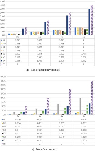
As expected, Figure 2 illustrates that the number of decision variables and constraints has increased as the size of instances increased. This figure shows that the numbers of periods, paths and nodes (including suppliers, manufacturers, whole-sellers and disposal centers) have the most significant impact on the number of decision variables. Moreover, the numbers of periods, whole-sellers and paths have the most prominent impact on the number of constraints. For instance, if we increase the number of periods based on Instance 5x, both the numbers of decision variables and constraints increases by 400% as compared to Instance x.

Furthermore, Figure 2 demonstrates that the numbers of first and second types of vehicles have the least impact on the number of decision variables. It also shows that the numbers of the first type of vehicles and disposal centers have the least impact on the number of constraints. To be more precise, if we increase the number of the first type of vehicles based on Instance 5x, the numbers of decision variables and constraints increases by 76.9% and 8.9% as compared to Instance x, respectively.

4. Numerical examples

4.1. Computational results

In this sub-section, 20 instances of various sizes are randomly generated and studied in order to validate the proposed mathematical formulation. It is noteworthy that we have stored all instances on the web at the address http://www.bitbucket.org/Pro_Data/instances_4. Accordingly, interested readers can apply these data for any future comparison.

To solve these instances using the CPLEX solver, we have coded the proposed model in GAMS 24.1.2. Then, we have run all these instances on a laptop with a Core i7 CPU and 8GB RAM. The specifications of these instances and the results obtained for them have been provided in Table 4. It should be noted that we have fixed a set of useless decision variables equal to zero in order to reduce the computational complexity of instances. For example, $\sum _{i\in \mathcal{M}}\sum _{j\in \mathcal{R}}$$\sum _{k\in }$_E$\sum _{p\in \mathcal{P}}\sum _{t\in \mathcal{T}}{x}_{ijkpt}=0$; this term states that no vehicle of the first type moves from manufacturers to whole-sellers. Based on our observation, fixing such decision variables to zero decreases the CPU time of instances.

Table 4. The results obtained for the instances.

	Specification
Instance	$\left|\mathcal{S}\right|$	$\left|\mathcal{M}\right|$	$\left|\mathcal{R}\right|$	$\left|\mathcal{D}\right|$	$|$E$|$	$\left|\mathcal{G}\right|$	$\left|\mathcal{T}\right|$	No. of variables	No. of constraints	Objective function	CPU time (min)	Optimality Status
1	1	2	3	1	2	3	2	1,078	332	78,176.63	0.017	Optimal
2	1	2	3	1	2	3	2	1,078	332	79,435.06	0.051	Optimal
3	1	2	4	1	2	4	2	1,664	584	98,855.00	0.527	Optimal
4	1	2	4	1	2	4	2	1,664	584	93,050.87	0.013	Optimal
5	1	2	4	2	2	4	2	2,088	610	88,889.88	0.666	Optimal
6	1	2	4	2	2	4	2	2,088	610	80,507.12	0.018	Optimal
7	1	2	5	2	2	4	2	2,560	802	139,897.69	0.734	Optimal
8	1	2	5	2	2	4	2	2,560	802	102,540.20	0.026	Optimal
9	2	2	5	1	3	4	3	4,470	1,227	134,532.64	5.764	Optimal
10	2	2	5	1	3	4	3	4,470	1,227	149,999.18	1.988	Optimal
11	2	3	6	1	3	6	3	8,172	2,349	177,445.68	4.833	Optimal
12	2	3	6	1	3	6	3	8,172	2,349	154,605.47	0.533	Optimal
13	2	3	6	2	4	6	3	10,608	2,436	162,710.24	11.121	Optimal
14	2	3	6	2	4	6	3	10,608	2,436	177,828.94	9.152	Optimal
15	2	3	7	2	4	8	3	14,700	3,930	175,661.49	17.238	Optimal
16	2	3	7	2	4	8	3	14,700	3,930	194,864.93	14.123	Optimal
17	2	3	8	2	5	10	4	28,020	7,928	276,904.27	29.801	Optimal
18	2	3	8	2	5	10	4	28,020	7,928	253,935.82	31.001	Optimal
19	2	4	8	3	6	12	4	42,976	9,876	270,500.67	75.371	Optimal
20	2	4	8	3	6	12	4	42,976	9,876	273,304.90	66.235	Optimal

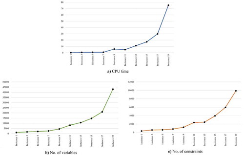
As shown in Table 4, all instances have been solved to optimality with small CPU times. The increment in the size of instances has increased the CPU times, where the largest instance has been solved to optimality in 75.371 minutes.

To better analyze how the complexity of these instances increases, we have compared the CPU times, and the number of decision variables and constraints. Figures 3(a–c) illustrate how the CPU time and the number of decision variables and constraints increase by the increment in the size of instances, respectively. As shown in Figure 3(a), the CPU time increases almost linearly for smaller size instances. Likewise, the numbers of decision variables and constraints increased with a similar trend. However, for larger size instances, the increment in the size of instances could considerably increase the CPU time. Even considering this issue, we preferred to merely apply the CPLEX solver rather than a heuristic/meta-heuristic algorithm. To support this idea, it can be argued that the solutions provided by the CPLEX solver (even with considerable CPU time) are high-quality. Furthermore, this paper studies a mid-term decision-making problem; thus, small CPU times are not crucial.

Figure 3. The comparison between the CPU Time, and number of decision variables and constraint.

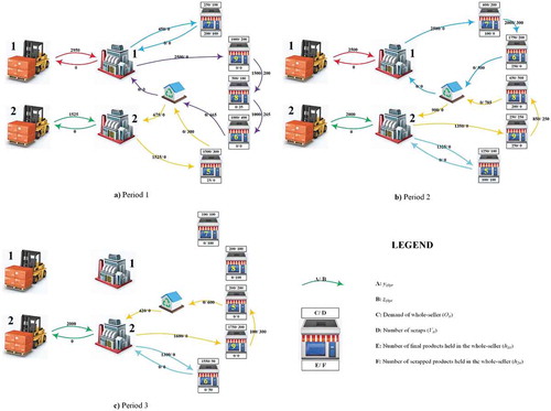
Figure 4 depicts the flow of final products and scraps through the CLCS designed for Instance 9. As illustrated in Figure 4, the demand of all whole-sellers has been completely satisfied over all periods, and all scraps have been collected until the last period.

Figure 4. Schematic representation of solution obtained for Instance 9.

4.2. Sensitivity analysis

In this section, we aim to analyze the five features of this problem. First, we have evaluated the effect of symmetry-breaking constraints on CPU time. Then, we have studied the impact of multi-path setting on the solutions. We have also studied how fixed costs of vehicles and the heterogeneous fleet of vehicles affect the solutions provided for this problem. Finally, we want to figure out how whole-sellers would react in a case that they could lose a portion of their demands (i.e. lost sales).

4.2.1. Symmetry-breaking constraints and CPU time

In sub-section 2.3, we introduced two symmetry-breaking constraints for vehicles of suppliers and manufacturers. These constraints aim to reduce the CPU time of the CPLEX solver for this problem. Accordingly, we want to evaluate how these two constraints affect the CPU time. For this reason, we have defined two cases. First, we have solved Instances 1, 3, 5, 7, 9, 11, 13, 15, 17 and 19 in the presence of the symmetry-breaking constraints (we call this case as the original case in the rest of paper). While in another case called as Case 1, we have eliminated those two constraints and recorded the CPU times of instances mentioned above. The obtained results have been illustrated in Figure 5. This figure shows the ratio of the CPU time obtained for each case to the sum of CPU times for an instance in both cases.

Figure 5. The impact of symmetry-breaking constraints on the CPU time.

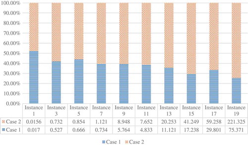
Figure 5 illustrates that including the symmetry-breaking constraints in the mathematical model can reduce the CPU time of all instances (except Instance 1). This figure also shows that the symmetry-breaking constraints affect the CPU time of larger size instance more significantly. To be more precise, the CPU time of Instance 19 has increased by about 193% in Case 1 as compared to the original case. Thus, it can be argued that adding the symmetry-breaking constraints can improve the efficiency of the CPLEX solver with respect to the CPU time.

4.2.2. Single- and multi-path settings

As previously indicated, this paper studies the multi-path setting between nodes. To analyze the impact of this feature on the quality of solutions, especially in terms of the variable costs of transportation, we have modified Instance 19 and created its single-path counterpart. It is evident that in the single-path setting, there is merely one path between every two nodes. To convert Instance 19 into a single-path instance, for nodes with more than one path, we have recognized the shortest path between all nodes of this instance and selected them. Finally, we have solved Instance 19 based on both single- and multi-path settings. The obtained results have been provided in Table 5.

Table 5. Comparison between the results of single- and multi-path settings.

	Total distance traveled (km)	Fixed cost of using vehicles	Variable cost of vehicles	Holding cost	Total cost
Single-path setting	10,787.82	28,500	274,294	2,283.10	305,077.10
Multi-path setting	10,967.53	28,500	238,242.10	3,758.57	270,500.67

According to Table 5, the total costs for the multi-path setting is significantly less as compared to the single-path setting, about 11.33%. For both single- and multi-path settings an equal number of vehicles has been used (i.e. equal fixed cost of using vehicles). Moreover, the total distance traveled for the single-path setting is less than the multi-path setting. However, Table 5 shows that the variable cost of vehicles is much less for the multi-path setting. For this setting, the variable cost of using vehicles is equal to 238,242.10, which is 36,051.9 unit (about 13.14%) less than the single-path setting. This implies that traveling shorter paths, which is used in the single-path setting, does not guarantee less fuel and car depreciation costs due to different road roughness degrees. A longer path between two nodes may incur less variable cost due to its better road condition (i.e. less road roughness). Therefore, considering multi-path setting and road roughness degree is a crucial feature for this problem and lets decision makers make better decisions.

4.2.3. Fixed cost

The next feature to analyze is the fixed cost of using vehicles. To study this feature, we have solved Instance 19 where there is no fixed cost for using vehicles (i.e. Case 2). Then, we have compared the results obtained for Case 2 with the ones obtained for the original case (i.e. a solution in which the fixed cost has been considered). The comparison of these two cases has been provided in Table 6. As indicated in this table, the number of first and second types of vehicles used in Case 2 has increased by 28.6% and 33.3%, respectively. Table 6 demonstrates that the costs of this CLSC excluding the fixed cost of vehicles in Case 2 has decreased by 2.2% as compared to the original case. This decrement is the result of acquiring more vehicles (more flexibility in satisfying whole-sellers’ demands). However, if using vehicles incurred fixed costs, according to Table 6, the fixed cost of using vehicles in Case 2 could have been equal to 37,500 units, which is 31.6% more than the fixed cost in the original case. Finally, this table shows that the total costs in Case 2 have increased by 2.5% as compared to the original case. To sum up, applying the fixed cost of using vehicles forces the mathematical model decrease the number of vehicles used to satisfy the demand of whole-sellers and reduces the whole costs of the system.

Table 6. The obtained results for the original case and Case 2.

	The original case		Case 2
Period	Between $\mathcal{S}$ and $\mathcal{M}$	Between $\mathcal{M}$, $\mathcal{R}$ and $\mathcal{D}$	Between $\mathcal{S}$ and $\mathcal{M}$	Between $\mathcal{M}$, $\mathcal{R}$ and $\mathcal{D}$
Period 1	3	5	3	7
Period 2	2	5	2	6
Period 3	1	4	2	6
Period 4	1	4	2	5
Total	7	18	9	24
Variable cost of using vehicles	238,242.10		235,975.79
Fixed cost of using vehicles	28,500		37,500
Sum of the fixed and variable costs	266,742.10		273,475.79

4.2.4. The heterogeneous fleet of vehicles

The third feature to analyze is the impact of the heterogeneous fleet of vehicles. To investigate this feature, we have solved Instance 19 where the first type of vehicles has been used throughout the CLSC design (i.e. Case 3), and the second type of vehicles has been used throughout the CLSC design (i.e. Case 4). Afterward, Cases 3 and 4 have been compared with the original case. The comparison of these three cases has been provided in Table 7. According to this table, the total number of vehicles used in Case 3 has decreased by 16% as compared to the original case since the capacity of the first type of vehicles is greater than the second type of vehicles. Nevertheless, the fixed cost of vehicles in Case 3 has increased by 10.5%; this increment has happened because the fixed cost of the first type of vehicles is 1.5 times greater than the second type of vehicles. Furthermore, Table 7 shows that the variable cost of vehicles in Case 3 has been increased by 43.6% as compared to the original case. This is because the variables cost of the first type of vehicles is higher than the second type. This table also shows that only using the second type of vehicles (i.e. Case 4) increases the total costs of this instance as compared to the original case. In Case 4, the total number of vehicles used to satisfy the demand of whole-sellers has increased by 47.6% as compared to the original case. This is because the capacity of the second type of vehicles is less than the first type of vehicles. Table 7 shows that the variable costs of vehicles in Case 4 has also been increased by 3.6% as compared to the original case.

Table 7. The obtained results for the original case and Cases 3 and 4.

Case	No. of vehicles used to satisfy the demands	Fixed cost of using vehicles	Variable cost of vehicles	Holding cost	Total costs
The original case	25	28,500	238,242.10	3,758.57	270,500.67
Case 3	21	31,500	342,044.32	2,221.43	380,265.75
Case 4	31	31,000	247,699.74	1,566.43	280,266.17

Based on the results provided for both Cases 3 and 4, it can be concluded that the heterogeneous fleet of vehicles is crucial for this problem and could improve the quality of solutions.

4.4.5. Lost sales

Finally, we want to study the impact of lost sales on this problem. To study this feature, we have solved Instance 19 where lost sales could occur with a penalty. We have replaced Constraint (10) with Constraints (32–35) in order to make lost sales possible for the model.

(32) $\begin{array}{rl}& l_{it}=O_{it}-\sum _{j\in \mathcal{M}}\sum _{k\in \mathcal{G}}\sum _{p\in \mathcal{P}}{y}_{jikpt}-\sum _{j\in \mathcal{R}}\sum _{k\in \mathcal{G}}\sum _{p\in \mathcal{P}}{y}_{jikpt}\\ & +\sum _{j\in \mathcal{R}}\sum _{k\in \mathcal{G}}\sum _{p\in \mathcal{P}}{y}_{ijkpt}+h_{1it}-h_{1i\left(t-1\right)}\mathrm{\forall }i\in \mathcal{R};t\in \mathcal{T}\end{array}$(32)

(33) $l_{it}\le n_{1it}{M}_1\mathrm{\forall }i\in \mathcal{R};t\in \mathcal{T}$(33)

(34) $h_{1it}\le n_{2it}{M}_2\mathrm{\forall }i\in \mathcal{R};t\in \mathcal{T}$(34)

(35) $n_{1it}+n_{2it}\le 1\mathrm{\forall }i\in \mathcal{R};t\in \mathcal{T}$(35)

where $l_{it}$ refers to the lost sales occurred in node $i$ ($i\in \mathcal{R}$) at period $t$; $n_{1it}$ and $n_{2it}$ are two auxiliary and binary decision variables. $M_1$ and $M_2$ also refer to two adequately large numbers. To be more precise, Constraint (32) creates a trade-off between lost sales, demand, input and output flows of final products and the amount of inventory held in node $i$ at period $t$. Constraints (33–35) ensures that node $i$ can only hold inventory or lost a portion of its demand at period $t$.

In Constraints (33 and 34), two adequately large coefficients (i.e. $M_1$, and $M_2$) exist that can activate these constraints when required. With small values chosen for $M_1$ and $M_2$, infeasible solutions may be generated; with very large values chosen for them, round-off error would occur. Consequently, it is important to choose suitable values for them. $M_1$ is used in Constraint (33). This constraint determines how much the demand of whole-sellers could be lost. Since $l_{it}$ can at most be equal to $\underset{i,t}{max}\left(O_{it}\right)$, thus, we set $M_1$ equal to $\underset{i,t}{max}\left(O_{it}\right)$. $M_2$ is also used in Constraint (34). This constraint determines how much a whole-seller can hold inventory. Since $h_{1it}$ can at most be equal to $\underset{i}{max}\left(C{F}_i\right)$, therefore, we have set $M_2$ equal to $\underset{i}{max}\left(C{F}_i\right)$. The values of these coefficients have been summarized in Table 8.

Table 8. The values of coefficients $M_1$ and $M_2$.

Coefficients	Values
$M_1$	$\underset{i,t}{max}\left(O_{it}\right)$
$M_2$	$\underset{i}{max}\left(C{F}_i\right)$

Table 9 compares the obtained results for Case 5 (where lost sales are allowed) and the original case. In Case 5, around 10% of the demand of whole-sellers have not been satisfied; whereas, the entire demands of whole-sellers have been satisfied in the original case. Accordingly, the lost sales cost of Case 5 is much higher than the original case. On the other hand, Table 9 shows that all other types of costs in Case 5 are less than the original case. This is rational since fewer final products have been transported to manufacturers, and to whole-sellers. It means that fewer vehicles have been used for transportation, less distance has been traveled, and less inventory has been held. Note that if we increase the penalty for each unit of lost sales, the model will satisfy more demands of whole-sellers over all periods. In other words, the model in Case 5 approaches the original case if we increase the value of the penalty coefficient.

Table 9. The obtained results for the original case and Case 5.

Case	Percentage of demands satisfied over all periods (%)	Lost sale cost	Fixed cost of using vehicles	Variable cost of vehicles	Holding cost	Total costs
The original case	100	0	28,500	238,242.10	3,758.57	270,500.67
Case 5	90	24,950	23,000	207,759.31	2,105	257,859.31

5. Conclusions and remarks

In this paper, the inventory-routing problem was studied for a CLSC. This CLSC includes suppliers, manufacturers, whole-sellers, and disposal centers. A mathematical model was proposed, which minimizes the total costs of a CLSC including the fixed and variable costs of using vehicles and holding inventory costs of final products and scraps. In this model, the road roughness degree and multi-path setting were studied, simultaneously. Furthermore, the heterogeneous fleet of vehicles between echelons was investigated, where the capacity of vehicles is limited, and the number of vehicles is finite.

First, the complexity of the mathematical model was assessed based on the number of variables and constraints. The results demonstrated that the numbers of periods, paths and nodes have the most significant impact on the number of decision variables. Moreover, the numbers of periods, whole-sellers and paths have the most prominent impact on the number of constraints. Second, to assess the integrity and validation of the proposed model, the authors generated 20 instances of different sizes. Then, they applied GAMS to code the mathematical model and solve all instance using the CPLEX solver. The computational results showed that the CPLEX solver could solve all instances to optimality in less than 100 minutes. Afterward, the authors illustrated the solution of an instance (i.e. Instance 9) and showed the validation of the model.

Then, a comprehensive sensitivity analysis was conducted to study five features of this paper. First, the impact of the symmetry-breaking constraints on the CPU time was studied. The results demonstrated that implementing these constraints could potentially decrease the CPU time by 73.9% on average. Second, the authors studied the impact of the multi-path setting on this problem. For this reason, they compared the results obtained for single- and multi-path settings. It became clear that traveling shorter distance does not necessarily reduce the variable costs of using vehicles. In other words, traveling longer paths may be more favorable as compared to the shorter ones due to lower road roughness degrees. Third, the impact of the fixed cost on using vehicles was studied. The results indicated that considering this type of cost could decrease the number of vehicles used to satisfy the demand of whole-sellers significantly. Then, the authors analyzed the effect of the heterogeneous fleet of vehicles on the quality of solutions. The results showed that using the homogenous fleet of vehicles (i.e. large or small vehicles) deteriorates the quality of solutions. While using the heterogeneous fleet of vehicles (i.e. a combination of large and small vehicles) increases the flexibility of the mathematical model and decreases the total costs of the CLSC (both the fixed and variable costs of using vehicles) significantly. Finally, the sensitivity analysis studied the impact of lost sales on this problem. The results demonstrated that the total costs of Instance 19 decreases by 4.7% where lost sales are possible; whereas 10% of the demand of whole-sellers were not satisfied.

Based on what was mentioned earlier, the main managerial implications of this study are as follows:

• Paths between two specific nodes may vary with respect to their length and road roughness degree. Traveling shorter paths are not always the best choice. To make the best decision, it is crucial to consider the impact of the length of paths and their road roughness degree.

• The heterogeneous fleet of vehicles will increase the flexibility of decision makers so that both the number of used vehicles and transportations costs remain low.

For the future research, we think that the development of a meta-heuristic algorithm would be valuable for larger size instances. Furthermore, studying the inherent uncertainties, e.g. uncertainty in demand of whole-sellers, might also be interesting.

Disclosure statement

No potential conflict of interest was reported by the authors.

Additional information

Notes on contributors

Amirhossein Moosavi

Amirhossein Moosavi has received his MSc and BSc from the IAU Karaj Branch at Industrial Engineering. He has published some papers in some of the most reputable journals of Management Science, like Computers & Industrial Engineering. His interest research area consists of the applications of operations research, scheduling, supply chain management, healthcare decision-making and heuristic/metaheuristic algorithms.

Adel Nikfarjam

Adel Nikfarjam got his BSc in industrial Engineering at the Azad University of Qazvin (QIAU); in addition, he got his MSc in Industrial Engineering at the IAU Karaj Branch. His research interests are Supply Chain, Inventory management, and Transportation. At the present time he is an employee in a Private Company.

References

- Aalaei, A., and H. Davoudpour. 2017. “A Robust Optimization Model for Cellular Manufacturing System into Supply Chain Management.” International Journal of Production Economics 183: 667–679. doi:10.1016/j.ijpe.2016.01.014.
- Alhaj, M. A., D. Svetinovic, and A. Diabat. 2016. “A Carbon-Sensitive Two-Echelon-Inventory Supply Chain Model with Stochastic Demand.” Resources, Conservation and Recycling 108: 82–87. doi:10.1016/j.resconrec.2015.11.011.
- Alimoradi, A. R., M. Yussuf, N. B. Ismail, and N. Zulkifli. 2015. “Developing a Fuzzy Linear Programming Model for Locating Recovery Facility in a Closed Loop Supply Chain.” International Journal of Sustainable Engineering 8 (2): 122–137. doi:10.1080/19397038.2014.906514.
- Alimoradi, A. R., M. Yussuf, and N. Zulkifli. 2011. “A Hybrid Model for Remanufacturing Facility Location Problem in A Closed-Loop Supply Chain.” International Journal of Sustainable Engineering 4 (1): 16–23. doi:10.1080/19397038.2010.533793.
- Archetti, C., M. Christiansen, and M. Grazia Speranza. 2018. “Inventory Routing with Pickups and Deliveries.” European Journal of Operational Research 268 (1): 314–324. doi:10.1016/j.ejor.2018.01.010.
- Bazan, E., M. Y. Jaber, and S. Zanoni. 2017. “Carbon Emissions and Energy Effects on a Two-Level Manufacturer-Retailer Closed-Loop Supply Chain Model with Remanufacturing Subject to Different Coordination Mechanisms.” International Journal of Production Economics 183: 394–408. doi:10.1016/j.ijpe.2016.07.00.
- Choudhary, A., S. Sarkar, S. Settur, and M. K. Tiwari. 2015. “A Carbon Market Sensitive Optimization Model for Integrated Forward–Reverse Logistics.” International Journal of Production Economics 164: 433–444. doi:10.1016/j.ijpe.2014.08.015.
- Denton, B. T., A. J. Miller, H. J. Balasubramanian, and T. R. Huschka. 2010. “Optimal Allocation of Surgery Blocks to Operating Rooms under Uncertainty.” Operations Research 58 (4–part–1): 802–816. doi:10.1287/opre.1090.0791.
- Du, S. F., M. Z. Fu, L. Zhu, and J. Zhang. 2015. “Game-Theoretic Analysis for an Emission-Dependent Supply Chain in a ‘Cap-And-Trade’ System.” Annals of Operations Research 228 (1): 135–149. doi:10.1007/s10479-011-0964-6.
- Fahimnia, B., M. Reisi, T. Paksoy, and Ö. Eren. 2013a. “The Implications of Carbon Pricing in Australia: An Industrial Logistics Planning Case Study.” Transportation Research Part D: Transport and Environment 18: 78–85. doi:10.1016/j.trd.2012.08.006.
- Fahimnia, B., J. Sarkis, A. Choudhary, and A. Eshragh. 2015. “Tactical Supply Chain Planning under A Carbon Tax Policy Scheme: A Case Study.” International Journal of Production Economics 164: 206–215. doi:10.1016/j.ijpe.2014.12.015.
- Fahimnia, B., J. Sarkis, F. Dehghanian, N. Banihashemi, and S. Rahman. 2013b. “The Impact of Carbon Pricing on a Closed-Loop Supply Chain: An Australian Case Study.” Journal of Cleaner Production 59: 210–225. doi:10.1016/j.jclepro.2013.06.056.
- Gentle, N. 1997. “Bass Strait freight rates-a decade after the Inter-State Commission inquiry”. In Australasian Transport Research Forum (ATRF), 21st, Adelaide, South Australia.
- Govindan, K., and H. Soleimani. 2017. “A Review of Reverse Logistics and Closed-Loop Supply Chains: A Journal of Cleaner Production Focus.” Journal of Cleaner Production 142: 371–384. doi:10.1016/j.jclepro.2016.03.126.
- Guide, V. D., and L. N. Wassenhove. 2006. “Closed‐Loop Supply Chains: An Introduction to the Feature Issue (Part 1).” Production and Operations Management 15: 345–350. doi:10.1111/j.1937-5956.2006.tb00249.x.
- Iassinovskaia, G., S. Limbourg, and F. Riane. 2017. “The Inventory-Routing Problem of Returnable Transport Items with Time Windows and Simultaneous Pickup and Delivery in Closed-Loop Supply Chains.” International Journal of Production Economics 183: 570–582. doi:10.1016/j.ijpe.2016.06.024.
- Jena, S. K., and S. P. Sarmah. 2016. “Future Aspect of Acquisition Management in Closed-Loop Supply Chain.” International Journal of Sustainable Engineering 9 (4): 266–276. doi:10.1080/19397038.2016.1181120.
- Kannan, D., A. Diabat, M. Alrefaei, K. Govindan, and G. Yong. 2012. “A Carbon Footprint Based Reverse Logistics Network Design Model.” Resources, Conservation and Recycling 67: 75–79. doi:10.1016/j.resconrec.2012.03.005.
- Kara, I., G. Laporte, and T. Bektas. 2004. “A Note on the Lifted Miller–Tucker–Zemlin Subtour Elimination Constraints for the Capacitated Vehicle Routing Problem.” European Journal of Operational Research 158 (3): 793–795. doi:10.1016/S0377-2217(03)00377-1.
- Kaya, O., and B. Urek. 2016. “A Mixed Integer Nonlinear Programming Model and Heuristic Solutions for Location, Inventory and Pricing Decisions in A Closed Loop Supply Chain.” Computers & Operations Research 65: 93–103. doi:10.1016/j.cor.2015.07.005.
- Keshari, A., N. Mishra, N. Shukla, S. McGuire, and S. Khorana. 2017. “Multiple Order-Up-To Policy for Mitigating Bullwhip Effect in Supply Chain Network.” Annals of Operations Research 269 (1–2): 361–386. doi:10.1007/s10479-017-2527-y.
- Kuo, T. C. 2011. “The Study of Production and Inventory Policy of Manufacturing/Remanufacturing Environment in a Closed-Loop Supply Chain.” International Journal of Sustainable Engineering 4 (4): 323–329. doi:10.1080/19397038.2011.593008.
- Margot, F. 2003. “Exploiting Orbits in Symmetric ILP.” Mathematical Programming 98 (1): 3–21. doi:10.1007/s10107-003-0394-6.
- Mawandiya, B. K., J. K. Jha, and J. Thakkar. 2016. “Two-Echelon Closed-Loop Supply Chain Deterministic Inventory Models in a Batch Production Environment.” International Journal of Sustainable Engineering 9 (5): 315–328. doi:10.1080/19397038.2015.1128495.
- Mohammed, F. S., Z. Selim, A. Hassan, and M. N. Syed. 2017. “Multi-Period Planning of Closed-Loop Supply Chain with Carbon Policies under Uncertainty.” Transportation Research Part D: Transport and Environment 51: 146–172. doi:10.1016/j.trd.2016.10.033.
- Rahimi, M., A. Baboli, and Y. Rekik. 2017. “Multi-Objective Inventory Routing Problem: A Stochastic Model to Consider Profit, Service Level and Green Criteria.” Transportation Research Part E: Logistics and Transportation Review 101: 59–83. doi:10.1016/j.tre.2017.03.001.
- Rahmani, D., and V. Mahoodian. 2017. “Strategic and Operational Supply Chain Network Design to Reduce Carbon Emission Considering Reliability and Robustness.” Journal of Cleaner Production 149: 607–620. doi:10.1016/j.jclepro.2017.02.068.
- Rakke, J. G., C. R. Magnus Stålhane, M. C. Moe, H. Andersson, K. Fagerholt, and I. Norstad. 2011. “A Rolling Horizon Heuristic for Creating A Liquefied Natural Gas Annual Delivery Program.” Transportation Research Part C: Emerging Technologies 19 (5): 896–911. doi:10.1016/j.trc.2010.09.006.
- Savaskan, R. C., S. Bhattacharya, and L. N. V. Wassenhove. 2004. “Closed-Loop Supply Chain Models with Product Remanufacturing.” Management Science 50 (2): 239–252. doi:10.1287/mnsc.1030.0186.
- Shankar, R., S. Bhattacharyya, and A. Choudhary. 2018. “A Decision Model for A Strategic Closed-Loop Supply Chain to Reclaim End-Of-Life Vehicles.” International Journal of Production Economics 195: 273–286. doi:10.1016/j.ijpe.2017.10.005.
- Sinha, K. C., and S. Labi. 2007. Transportation Decision Making Principles of Project Evaluation and Programming. Hoboken: John Wiley.
- Soysal, M. 2016. “Closed-Loop Inventory Routing Problem for Returnable Transport Items.” Transportation Research Part D: Transport and Environment 48: 31–45. doi:10.1016/j.trd.2016.07.001.
- Soysal, M., J. M. Bloemhof-Ruwaard, R. Haijema, and V. D. V. Jack G. A. J. 2015. “Modeling an Inventory Routing Problem for Perishable Products with Environmental Considerations and Demand Uncertainty.” International Journal of Production Economics 164: 118–133. doi:10.1016/j.ijpe.2015.03.008.
- Stålhane, M. J., G. Rakke, C. R. Moe, H. Andersson, M. Christiansen, and K. Fagerholt. 2012. “A Construction and Improvement Heuristic for A Liquefied Natural Gas Inventory Routing Problem.” Computers & Industrial Engineering 62 (1): 245–255. doi:10.1016/j.cie.2011.09.011.
- Talaei, M., B. F. Moghaddam, M. S. Pishvaee, A. Bozorgi-Amiri, and S. Gholamnejad. 2016. “A Robust Fuzzy Optimization Model for Carbon-Efficient Closed-Loop Supply Chain Network Design Problem: A Numerical Illustration in Electronics Industry.” Journal of Cleaner Production 113: 662–673. doi:10.1016/j.jclepro.2015.10.074.
- Tao, Z. G., Z. Y. Guang, S. Hao, H. J. Song, and D. G. Xin. 2015. “Multi-Period Closed-Loop Supply Chain Network Equilibrium with Carbon Emission Constraints.” Resources, Conservation and Recycling 104: 354–365. doi:10.1016/j.resconrec.2015.07.016.
- Tosarkani, B. M., and S. H. Amin. 2018. “A Possibilistic Solution to Configure A Battery Closed-Loop Supply Chain: Multi-Objective Approach.” Expert Systems with Applications 92: 12–26. doi:10.1016/j.eswa.2017.09.039.
- Üster, H., and S. O. Hwang. 2017. “Closed-Loop Supply Chain Network Design under Demand and Return Uncertainty.” Transportation Science 51 (4): 1063–1085. doi:10.1287/trsc.2015.0663.
- Zakeri, A., F. Dehghanian, B. Fahimnia, and J. Sarkis. 2015. “Carbon Pricing versus Emissions Trading: A Supply Chain Planning Perspective.” International Journal of Production Economics 164: 197–205. doi:10.1016/j.ijpe.2014.11.012.
- Zhang, Y., H. Alshraideh, and A. Diabat. 2018. “A Stochastic Reverse Logistics Production Routing Model with Environmental Considerations.” Annals of Operations Research 271 (2): 1023–1044. doi:10.1007/s10479-018-3045-2.