A novel approach integrating FANP and MOMILP for the collection centre location problem in closed-loop supply chain

ABSTRACT

Supply chain network design plays a crucial role in supply chain management. With government support as well as restriction and legislation, the enhancement of environmental awareness, and the drive of economic interest, reverse logistics have been incorporated into the supply chain, forming a closed-loop supply chain. The collection centre, which helps recycle and classify returned products, is a vital hub in closed-loop networks. Regarding the location problem, this study proposes a novel approach that integrates a fuzzy analysis network process and multi-objective mixed-integer linear programming to analyse qualitative and quantitative factors: social, political, and environmental factors, including costs, $C{O}_2$ emissions, and responsiveness. Hence, an ε-constraint method is applied to examine the proposed framework. Finally, uncertain scenarios and different scale problems are discussed. Orthogonal experiments provide a sufficient basis for decision-making.

KEYWORDS:

• Closed-loop supply chain
• multi-factor
• fuzzy analytic network process
• multi-objective mixed integer linear programming
• facility location

1. Introduction

Facility location problems (FLPs) are a key aspect of supply chain network designs. The simplest setting is the one in which p facilities are to be selected to minimise the total distances or costs for supplying customer demands (Melo, Nickel, and Saldanha-da-Gama 2009). Researchers and institutions have conducted numerous studies on this issue and put forward many location selection methods.

The site selection of collection centres is one FLP. The collection centre, as a vital hub of reverse logistics, is an important part of a closed-loop supply chain (CLSC). However, there are numerous factors affecting the location selection design. Thus, it becomes more difficult to analyse these qualitative or quantitative factors.

The location selection methods proposed by previous research can be divided into mathematical programming methods (MPMs) and system evaluation methods (SEMs). The former is usually used to calculate the quantitative factors and is optimised by objective functions, whereas the latter uses evaluation methods to analyse the pros and cons of candidates and is more used in the analysis of qualitative factors, which are difficult to be quantified.

Much of the existing literature focuses on only one of the aforementioned methods. The factors considered by MPMs are limited and must be quantified. However, in reality, many factors are difficult or even impossible to quantify. While SEMs can be used to consider a wide range of factors, they are somewhat subjective. Thus, the integration of the two methods can combine all types of factors to make superior decisions.

This paper proposes a novel approach to consider extensive factors and provide objective guidance for decision-making through the integration of fuzzy analysis network process (FANP) and multi-objective mixed-integer linear programming (MOMILP).

When solving the location problem, the impact of qualitative factors on a site and its costs are usually calculated by these two methods, respectively. Thus, as the intersection of two types of factors, the collection centre becomes the key element of the integration approach. In this paper, FANP will be used to evaluate qualitative factors. Then, evaluation values will be converted into penalty coefficients and integrated into the MOMILP to optimise location results.

Based on previous considerations, the remainder of this paper is organised as follows. Section 2 provides an overview of some of the most advanced studies on FLPs. The integrated approach is described in detail in Section 3. Section 4 presents a mathematical framework that considers all factors. Section 5 presents numerical examples and discusses computational results. Finally, we draw conclusions in Section 6.

2. Literature review

The supply chain has always been a hot topic in the logistics industry, and Figure 1 shows a general case of a CLSC network structure, covering a variety of roles in the supply chain and three methods of recycling (Govindan, Soleimani, and Kannan 2015). Facility location is part of the strategic planning of a supply chain and constitutes part of the network structure. On this basis, multiple goals or factors are considered; different methods were used to evaluate these factors.

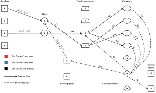
Figure 1. A generic closed-loop supply chain network.

2.1. Mathematical programming methods

In MPMs, mathematical models are constructed to optimise various factors; among these, cost is a common factor to be considered. Özceylan and Paksoy (2013) discussed costs in multiple scenarios. Alimoradi et al. (2015) used fuzzy MILP to consider the uncertainty of costs and demands. Additionally, the focus of researches has gradually expanded to more factors. Multi-objective programming (MOP) appears in MPMs.

Pishvaee, Farahani, and Dullaert (2010) developed a bi-objective model to optimise the total costs and responsiveness of a logistics network. A new search algorithm is utilised and compared to Pareto-optimal solutions. Similarly, Ramezani, Bashiri, and Tavakkoli-Moghaddam (2013) demonstrated a method to maximise profit, customer responsiveness, and quality. Different level capacities of facilities are considered in the stochastic programming model and Pareto-optimal are also applied. These papers focus on the economic and service aspects. We can use some methods to quantify these goals. Furthermore, with the emphasis on environmental protection, many papers incorporate environmental factors into location optimisation goals. Pishvaee and Razmi (2012) also considered the cost of the supply chain and the impact on the environment and used fuzzy methods to solve uncertain problems. Govindan, Jha, and Garg (2016) attempted to maximise profit, save activity costs, and made a positive impact on societal development. The interactive MOP approach is used to adjust the weight of each target. Gradually, calculating $C{O}_2$ or fine dust emissions becomes a way to quantify environmental factors. Nagurney and Nagurney (2010) developed an analytical framework, they skillfully used different links to indicate different levels of capacity and emissions, ultimately optimising costs and emissions. Ebrahimi (2018) considered total costs, environmental emissions and the responsiveness. In particular, the quantity discount for purchases is considered in the model. Linearisation of the model is used to simplify the problem. This MOP was solved by ɛ-constraint and Pareto solution.

In summary, the impacts of different factors are quantitatively calculated by MOPs. The most common methods to deal with MOP use linearly weighted or ε-constraint to transform them into single-objective problems. Pareto optimisation is also often used to evaluate results. However, these MPMs have some limitations when considering more qualitative factors. The diversity of factors and the difficulty of quantification cause problems in terms of calculation.

2.2. System evaluation methods

SEMs have certain advantages, and the difficulty regarding calculation and optimisation is lower than that of MPMs. Therefore, it can handle multi-factor problems very well. Niroomand et al. (2018) considered factors such as distance, time, population of the zone, expected emergency calls semi-annually, and so on when considering the location of an emergency centre. They only used a non-linear model to determine the weight of the factors and then used the interval technique for order preference by similarity to an ideal solution (TOPSIS) to obtain the rank of candidate locations. The calculation difficulty in this paper is lower than that of MPMs. In Table 1, we present different factors and methods when selecting sites. According to this table, the following conclusions are made:

Table 1. Reviewed works of system evaluation methods.

Reference	Factors	Methods
(Chan et al. 2008)	Cost of Ownership, Quality, Service, Background, Risk factors.	FAHP
(Tabari et al. 2008)	Work culture, Climatic condition, Housing facility, Transportation availability, Recreational facility.	FAHP
(Kayikci 2010)	Environmental effect, International market location, Intermodal operation and management, National stability and economical scale.	FAHP
(Alimoradi, Yussuf, and Zulkifli 2011)	Closeness to manufacturers, Availability of machines and tools, Closeness to customers or demand points, Availability of proper logistics	Fuzzy-TOPSIS
(Kuo 2011)	Port rate, Import/Export volume, Location resistance, Extension transportation convenience, Transshipment time, One stop service, Information abilities, Port & warehouse facilities, Port operation system, Density of shipping line.	Fuzzy-DEMATEL AHP/ANP
(Roh, Jang, and Han 2013)	Location, Logistics, National Stability, Cost, Cooperation.	AHP
(Kabir and Sumi 2014)	Social factors, Technological factors, Economic factors, Environmental factors, Site characteristic.	FAHP, PROMETHEE
(Temur 2016)	Unit price, Stock holding capacity, Average distance to shops, Average distance to main suppliers, Movement flexibility.	CBDO
(Jatuphatwarodom, Jones, and Ouelhadj 2018)	Product quality, Service level, Management, Financial flow	DEA AHP EGP

• Most of the early studies used only one method. Later, researchers combined multiple methods for evaluation.

• More types of factors are considered in the systematic review method than in MPMs.

• Analytic hierarchy process (AHP) or FAHP is used most frequently.

In summary, SEMs can analyse the ranking of candidates under many factors, but decision-makers are unable to recognise the objective gap.

2.3. Integration approaches

We can see that only one type of method was used in many studies. While integration approaches combine various advantages, only a few studies combined both methods as done in current studies. Cheng, Chan, and Huang (2003) used MILP to calculate the minimum total cost of all optional locations, the multi-criteria decision analysis will then take the cost as one criterion to analyse. This integration approach is very clever, but it needs multiple calculations to analyse all alternative location schemes. Ozgen and Gulsun (2014) used FAHP to analyse qualitative factors, such as proximity to market and city planning, and its evaluation results will be one objective of MOP. Simultaneously, transportation and facilities costs were calculated using possibilistic linear programming and become another objective of MOP. However, when the site selection affects only a small portion of the supply chain network, for example, when the collection centre location mainly affects the reverse logistics network, it is difficult for MOP to measure the impact using an independent objective. This paper is different from the method in that the calculation of qualitative factors only affect the site selection facilities.

3. Approach definition

3.1. Problem description

The general structure of the CLSC is illustrated in Figure 1. In the forward logistics, components purchased from suppliers will be processed and assembled at plants to form the end-product which will be delivered to customers through distribution centres. In the reverse logistics, the collection centre plays a more vital role. The returned product collected from customers will be divided into three parts in the collection centre, and then processed through three different recycling methods: (1) The part which can be directly reused will be transported to distribution centres for resale. (2) The damaged part will be transported to the recovery plant for disassembly and refurbishing, and then provide components for plants to remanufacture. (3) The useless part is transported to the disposal centre for disposal.

This paper addresses the location design of collection centres. Opening a suitable number of collection centres makes location results optimal in all factors. In this paper, the following assumptions are made:

• All candidate sites of the collection centre and other facilities are known.

• The flow between facilities only occurs between two connected layers.

• The capacity of all facilities is known.

• All kinds of unit costs and emissions are known.

• The maximum number of opened collection centres are known.

3.2. The novel integration approach

We established MOMILP as an MPM and selected FANP from SEMs. The integration approach proposed in this paper is divided into four steps, and the framework is shown in Figure 2. The steps are as follows:

Figure 2. The solution framework of the integration approach.

1. Identifying all factors that affect the operation of collection centres. In this paper, qualitative factors include 10 sub-factors from three aspects: social, political, and environmental factors; quantitative factors include costs, $C{O}_2$ emissions, and responsiveness.

2. Using FANP to evaluate qualitative factors of candidate sites.

3. The evaluation results are converted into a penalty coefficient to increase the fixed costs of candidate sites and increase the unit transportation cost when products flow through the candidate site.

4. These new cost parameters with penalty values are taken into the MOMILP for location optimisation.

4. Multi-factor methodology

4.1. Factors and settings

Considering the qualitative factors, this paper refers to the factors proposed by different researchers in Table 1. These factors show in Figure 3(a). Social factors include the impact of different social conditions on the collection centre, such as public facilities conditions ($E_1$) and safety ($E_2$) and talents reserve ($E_3$), as well as the impact of the collection centre on the community, such as the impact on the lives of residents ($E_4$) and the impact on traffic ($E_5$). Social factors represent the relationship between candidate sites and society. The political factors are related to relevant laws and regulations ($E_6$), and political stability ($E_7$). These factors take into account the policy guidance or subsidy from the local government for opening a collection centre. The environmental factors include the climate ($E_8$), geographical ($E_9$) and transportation line ($E_{10}$) conditions, and these factors have a greater impact on employees life. Among social factors, if there are more public facilities, such as more convenient public transportation facilities, it will facilitate the transportation of products. This will reduce the impact of collection centres on traffic jam. Ultimately, the impact on nearby residents will also be reduced. In environmental factors, climate and geographical location are often associated. In addition, there is no clear correlation between other factors. Therefore, these 10 factors can be constructed into a network structure which shows in Figure 3(b). It is composed of different clusters and elements that are connected with each other. These 10 factors are closely related to the operation of the collection centre. So, the evaluation score of these 10 factors can be used as a penalty coefficient to increase the fixed and transportation costs.

Figure 3. (a) Description of qualitative factors. (b) A network of connections between factors.

The quantitative factors are mainly reflected in three common goals: total costs, $C{O}_2$ emissions, and responsiveness. These factors are used to evaluate the overall supply chain performance.

To describe the aforementioned CLSC network, we use the following notations in the model formulations:

Sets:

$i$	=	Set of fixed suppliers
$j$	=	Set of fixed plants
$k$	=	Set of fixed distribution centres
$l$	=	Set of fixed customers
$m$	=	Set of potential collection centres
$n$	=	Set of fixed recovery plants
$d$	=	Set of fixed disposal centres
$c$	=	Set of components
$p$	=	Set of periods
$e$	=	Set of factors

Decision variables:

$QI{J}_{{ }_{ijc}}^p$	=	Quantity of component $c$ transported from supplier $i$ to plant $j$ in period p
$QJ{K}_{{ }_{jk}}^p$	=	Quantity of end-product transported from plant $j$ to distribution centre $k$ in period p
$QK{L}_{{ }_{kl}}^p$	=	Quantity of end-product transported from distribution centre $k$ to customer $l$ in period p
$QL{M}_{{ }_{lm}}^p$	=	Quantity of returned product transported from customer $l$ to collection centre $m$ in period p
$QM{K}_{{ }_{mk}}^p$	=	Quantity of directly reused product transported from collection centre $m$ to distribution centre $k$ in period p
$QM{N}_{{ }_{mn}}^p$	=	Quantity of recoverable product transported from collection centre $m$ to recovery plant $n$ in period p
$QM{D}_{{ }_{md}}^p$	=	Quantity of useless product transported from collection centre $m$ to disposal centre $d$ in period p
$QN{J}_{{ }_{njc}}^p$	=	Quantity of component $c$ transported from recovery plant $n$ to plant $j$ in period p
$H_{{ }_m}^p$	=	$=\left\{\begin{array}{c}1,\mathrm{I}\mathrm{f}\mathrm{c}\mathrm{o}\mathrm{l}\mathrm{l}\mathrm{e}\mathrm{c}\mathrm{t}\mathrm{i}\mathrm{o}\mathrm{n}\mathrm{c}\mathrm{e}\mathrm{n}\mathrm{t}\mathrm{e}\mathrm{r}m\mathrm{i}\mathrm{s}\mathrm{o}\mathrm{p}\mathrm{e}\mathrm{n}\mathrm{i}\mathrm{n}\mathrm{p}\mathrm{e}\mathrm{r}\mathrm{i}\mathrm{o}\mathrm{d}p,\\ 0,\mathrm{o}\mathrm{t}\mathrm{h}\mathrm{e}\mathrm{r}\mathrm{w}\mathrm{i}\mathrm{s}\mathrm{e};\end{array}\right\}$

Parameters：

$w_e$	=	The weight of factor $e$ calculated by FANP
$v_{me}$	=	The evaluation score of the collection centre $m$ on the factor $e$
$a_m$	=	The FANP evaluation value of the collection centre $m$
$pr$	=	The ratio of subjective importance of all qualitative factors in all factors $pr\in (0,1)$
$C{I}_{ic}$	=	Capacity of supplier $i$ for component $c$
$C{J}_j$	=	Capacity of plant $j$
$C{K}_k$	=	Capacity of distribution centre $k$
$D_l^p$	=	Demand of customer $l$ in period p
$C{M}_m$	=	Capacity of collection centre $m$
$C{N}_{nc}$	=	Capacity of recovery plant $n$ for component $c$
$d{i}_{ij}$	=	Distance between supplier $i$ and plant $j$
$d{j}_{jk}$	=	Distance between plant $j$ and distribution centre $k$
$d{k}_{kl}$	=	Distance between distribution centre $k$ and customer $l$
$d{l}_{lm}$	=	Distance between customer $l$ and collection centre $m$
$dm{n}_{mn}$	=	Distance between collection centre $m$ and recovery plant $n$
$dm{k}_{mn}$	=	Distance between collection centre $m$ and distribution centre $k$
$dm{d}_{md}$	=	Distance between collection centre $m$ and disposal centre $d$
$dn{j}_{nj}$	=	Distance between recovery plant $n$ and plant $j$
$r_c$	=	The utilisation rate of component $c$ in a unit end-product
${\alpha }_m$	=	Fixed cost for opening collection centre $m$
$t$	=	Unit cost of transportation
$C{O}_{2t}$	=	Unit $C{O}_2$ emission of transportation
$C{O}_{2s}$	=	Unit $C{O}_2$ emission of purchasing components
$C{O}_{2p}$	=	Unit $C{O}_2$ emission of producing an end-product.
$C{O}_{2r}$	=	Unit $C{O}_2$ emission of recovery component
$C{O}_{2d}$	=	Unit $C{O}_2$ emission of disposal
$C{O}_{2m}$	=	$C{O}_2$ emission for opening collection centre $m$
$S{C}_{ic}$	=	Unit cost of purchasing of supplier $i$ component $c$
$P{C}_j$	=	Unit cost of production of plant $j$
$R{C}_{nc}$	=	Unit cost of recovery plant $n$ for component $c$
$D{C}_d$	=	Unit cost of disposal of disposal centre $d$
$H_{max}$	=	Maximum number of opening collection centre
$\eta$	=	Return ratio of used product at customers
$\theta$	=	Direct reuse ratio
$\lambda$	=	Recovery ratio
$\beta$	=	The weighting coefficient for the forward responsiveness

4.2. Qualitative factor penalty value calculation

In order to get the penalty coefficient from qualitative factors, this paper follows the below steps. Firstly, the qualitative factors are analysed by FANP to get weights $w_e$ and scores $v_{me}$. Subsequently, evaluation results $a_m$ will be calculated by linearly weighted:

(1) $a_m=\sum _e{w}_e\cdot v_{me}$(1)

If the evaluation value $a_m$ is bigger, it proves that the candidate is more dominant in qualitative factors. Then, it will be transformed as using the Min-Max normalisation Equation(2) ${\hat{a}}_m=(1-pr)+\frac{pr}{a_{(n)}-a_{(1)}}\cdot (a_m-a_{(1)})$(2) (2), and the interval is $\left[1-pr,1\right]$.

(2) ${\hat{a}}_m=(1-pr)+\frac{pr}{a_{(n)}-a_{(1)}}\cdot (a_m-a_{(1)})$(2)

In Equation (2)(2) ${\hat{a}}_m=(1-pr)+\frac{pr}{a_{(n)}-a_{(1)}}\cdot (a_m-a_{(1)})$(2) , $a_{(n)}$ and $a_{(1)}$ are the order statistics of $a_m$, where $a_{(n)}$ is the maximum and $a_{(1)}$ is the minimum. The final result ${\hat{a}}_m$ is the penalty coefficient.

The qualitative factor penalty value will be calculated according to the Equation(3) $\mathrm{\Delta }{\alpha }_m=\left(\frac{1}{{\hat{\mathrm{a}}}_m}-1\right)\cdot {\alpha }_m;\mathrm{\Delta }{t}_m=\left(\frac{1}{{\hat{\mathrm{a}}}_m}-1\right)\cdot t$(3) (3). In this equation, the reciprocals of ${\hat{a}}_m$ claim that the candidate site with the larger evaluation value has smaller penalty values. And the penalty value is related to the original cost.

(3) $\mathrm{\Delta }{\alpha }_m=\left(\frac{1}{{\hat{\mathrm{a}}}_m}-1\right)\cdot {\alpha }_m;\mathrm{\Delta }{t}_m=\left(\frac{1}{{\hat{\mathrm{a}}}_m}-1\right)\cdot t$(3)

$\mathrm{\Delta }{\alpha }_m$ and $\mathrm{\Delta }{t}_m$ just represent the impact of qualitative factors on this collection centre. In the location optimisation, new cost parameters will be the sum of the penalty value and the original cost, which can be obtained by the Equation(4) ${\hat{\alpha }}_m={\alpha }_m+\mathrm{\Delta }{\alpha }_m;{\hat{t}}_m=t+\mathrm{\Delta }{t}_m$(4) (4).

(4) ${\hat{\alpha }}_m={\alpha }_m+\mathrm{\Delta }{\alpha }_m;{\hat{t}}_m=t+\mathrm{\Delta }{t}_m$(4)

Therefore, the bigger the qualitative score of the candidate site is, the smaller the penalty value will become. The same conclusion is as follows:

• The bigger the $pr$ is, the greater the ranges of $\mathrm{\Delta }\alpha$ and $\mathrm{\Delta }t$ will fluctuate.

• When qualitative factors are extremely important among all factors, $pr$ is infinitely close to 1. For the last candidate in the rank, $\underset{pr\to 1}{lim}{\hat{\alpha }}_{\left(1\right)}=+\mathrm{\infty }$ which shows the significant effect of qualitative factors. In contrast, for all candidate sites, $\underset{pr\to 0}{lim}{\hat{\alpha }}_m={\alpha }_m$ indicating that qualitative factors have no effect.

• When $pr=0.5$, $\mathrm{\Delta }{\alpha }_{(1)}=\alpha$. It shows that the penalty value of the last one is the same as the original cost, reflecting the same importance between qualitative factors and quantitative factors.

4.3. Model formulation

The results in 4.2 and other parameters are used to establish a MOMILP.

4.3.1. Objective functions

(5) $\begin{array}{rl}& Min{f}_{cost}=t\cdot \left(\sum _p\sum _i\sum _j\sum _{c}QI{J}_{ijc}^p\cdot d{i}_{ij}+\sum _p\sum _i\sum _{k}QJ{K}_{jk}^p\cdot d{j}_{jk}+\sum _p\sum _k\sum _{l}QK{L}_{kl}^p\cdot d{k}_{kl}\right.\\ & \left.+\sum _p\sum _n\sum _j\sum _{c}QN{J}_{njc}^p\cdot dn{j}_{nj}\right)+{\hat{t}}_m\cdot \left(\sum _p\sum _l\sum _{m}QL{M}_{lm}^p\cdot d{l}_{lm}+\sum _p\sum _m\sum _{k}QM{K}_{mk}^p\cdot dm{k}_{mk}\right.\\ & \left.+\sum _p\sum _m\sum _{n}QM{N}_{mn}^p\cdot dm{n}_{mn}+\sum _p\sum _m\sum _{d}QM{D}_{md}^p\cdot dm{d}_{md}\right)+\end{array}$(5)

(6) $\sum _p\sum _i\sum _j\sum _{c}QI{J}_{ijc}^p\cdot S{C}_{ic}+$(6)

(7) $\sum _p\sum _i\sum _{k}QJ{K}_{{ }_{jk}}^p\cdot P{C}_j$(7)

(8) $\sum _p\sum _n\sum _j\sum _{c}QN{J}_{njc}^p\cdot R{C}_{nc}+$(8)

(9) $\sum _p\sum _m\sum _{d}QM{D}_{md}^p\cdot D{C}_d+$(9)

(10) $\sum _p\sum _m{H}_m^p\cdot {\hat{\alpha }}_m$(10)

(11) $\begin{array}{rl}& Min{f}_{co2}=C{O}_{2t}\cdot \left(\sum _p\sum _i\sum _j\sum _{c}QI{J}_{ijc}^p+\sum _p\sum _i\sum _{k}QJ{K}_{jk}^p+\sum _p\sum _k\sum _{l}QK{L}_{kl}^p\right.\\ & +\sum _p\sum _n\sum _j\sum _{c}QN{J}_{njc}^p+\sum _p\sum _l\sum _{m}QL{M}_{lm}^p+\sum _p\sum _m\sum _{k}QM{K}_{mk}^p\\ & \left.+\sum _p\sum _m\sum _{n}QM{N}_{mn}^p+\sum _p\sum _m\sum _{d}QM{D}_{md}^p\right)+\end{array}$(11)

(12) $\sum _p\sum _i\sum _j\sum _{c}QI{J}_{ijc}^p\cdot C{O}_{2s}+$(12)

(13) $\sum _p\sum _i\sum _{k}QJ{K}_{{ }_{jk}}^p\cdot C{O}_{2p}$(13)

(14) $\sum _p\sum _n\sum _j\sum _{c}QN{J}_{njc}^p\cdot C{O}_{2\mathrm{r}}+$(14)

(15) $\sum _p\sum _m\sum _{d}QM{D}_{md}^p\cdot C{O}_{2d}+$(15)

(16) $\sum _p\sum _m{H}_m^p\cdot C{O}_{2m}^p$(16)

(17) $Max{f}_r=\sum _p\left(\beta \cdot \sum _k\frac{QK{L}_{kl}^p}{D_l^p}+(1-\beta )\cdot \sum _k\frac{QL{M}_{lm}^p}{\eta \cdot D_l^p}\right)$(17)

The goal of three objective functions is finding the appropriate location results and network logistics. In objective $f_{cost}$, the first part (5) is the total transportation cost. The parts(6) –(9) represent the costs in purchasing, production, recovery, and disposal, respectively. The last part (10) is the total fixed costs for opening the collection centre. Meanwhile, ${\hat{\alpha }}_m$ and ${\hat{t}}_m$, the new parameters with penalty values, are used in the calculation. As a result, the impacts of all qualitative factors can be incorporated into the objective. The second objective $f_{co2}$ seeks to minimise the environmental impact by the calculation of $C{O}_2$ emission. Similar to $f_{cost}$, parts(11) –(16) calculate emissions in various processes (transportation, production, etc.). The third objective $f_r$ seeks to maximise the responsiveness of the integrated network. Equation(17) $Max{f}_r=\sum _p\left(\beta \cdot \sum _k\frac{QK{L}_{kl}^p}{D_l^p}+(1-\beta )\cdot \sum _k\frac{QL{M}_{lm}^p}{\eta \cdot D_l^p}\right)$(17) (17) calculates the total responsiveness in all periods. It includes the demand satisfaction rate in the forward logistics and the recycling satisfaction rate in reverse logistics.

4.3.2. Constraints

Balance constraints:

(18) $\sum _{i}QI{J}_{ijc}^p+\sum _{n}QN{J}_{njc}^{p-1}-r_c\cdot \sum _{k}QJ{K}_{jk}^p=0,{\mathrm{\forall }}_{j,c,p}$(18)

(19) $\sum _{j}QJ{K}_{jk}^p+\sum _{m}QM{K}_{mk}^{p-1}-\sum _{l}QK{L}_{kl}^p=0,{\mathrm{\forall }}_{k,p}$(19)

(20) $\sum _{k}QK{L}_{kl}^p\ge D_{{ }_l}^p,{\mathrm{\forall }}_{l,p}$(20)

(21) $\eta \cdot \sum _{k}QK{L}_{kl}^p\le \sum _{m}QL{M}_{lm}^p\le D_{{ }_l}^p,{\mathrm{\forall }}_{l,p}$(21)

(22) $\theta \cdot \sum _{l}QL{M}_{lm}^p-\sum _{k}QM{K}_{mk}^p=0,{\mathrm{\forall }}_{m,p}$(22)

(23) $\lambda \cdot \sum _{l}QL{M}_{lm}^p-\sum _{d}QM{D}_{md}^p=0,{\mathrm{\forall }}_{m,p}$(23)

(24) $(1-\theta -\lambda )\cdot \sum _{l}QL{M}_{lm}^p-\sum _{n}QM{N}_{mn}^p=0,{\mathrm{\forall }}_{m,p}$(24)

(25) $r_c\cdot \sum _{m}QM{N}_{mn}^p-\sum _{j}QN{J}_{nj}^p=0,{\mathrm{\forall }}_{n,c,p}$(25)

These constraints keep that, for each product/component, the quantity entering each facility must be equal to the quantity leaving from this facility. Constraints(18) –(19) keep the balance in plants and distribution centres, respectively (contain the recycling products/components from the last period). Constraint (20) states that the flow exiting from distribution centres must be satisfied with the demands of all customers. The constraint (21) indicates that the quantity of return products entering collection centres must meet recycling demands. Constraints(22) –(24) represent three recycling methods and their ratios in returned products. Constraints (25) keeps the balance in recovery plants.

Capacity constraints:

(26) $\sum _{j}QI{J}_{ijc}^p\le C{I}_{ic},{\mathrm{\forall }}_{i,c,p}$(26)

(27) $\sum _{l}QJ{K}_{kl}^p\le C{J}_k,{\mathrm{\forall }}_{k,p}$(27)

(28) $\sum _{l}QK{L}_{kl}^p\le C{L}_k,{\mathrm{\forall }}_{k,p}$(28)

(29) $\sum _{l}QL{M}_{lm}^p\le C{M}_m,{\mathrm{\forall }}_{m,p}$(29)

(30) $\sum _{j}QN{J}_{njc}^p\le C{N}_{nc},{\mathrm{\forall }}_{n,c,p}$(30)

(31) $\sum _{m}QM{D}_{md}^p\le C{D}_d,{\mathrm{\forall }}_{d,p}$(31)

Capacity constraints ensure that the sum of the flow exiting from each facility to others does not exceed the capacity of this facility. Constraints(26) –(31) stipulate that the quantity of components/products not exceeds the capacities of suppliers, plants, distribution centres, collection centres, recovery plants, and disposal centres, respectively.

Range constraints:

(32) $\sum _m{H}_m^p\le H_{max},{\mathrm{\forall }}_p$(32)

(33) $H_m^p=\left\{0,1\right\},{\mathrm{\forall }}_{m,p}$(33)

(34) $QI{J}_{ijc}^p,QJ{K}_{jk}^p,QK{L}_{kl}^p,QL{M}_{lm}^p,QM{N}_{mn}^p,QM{K}_{mk}^p,QM{D}_{md}^p,QN{J}_{nj}^p\ge 0,{\mathrm{\forall }}_{i,j,k,l,m,n,d,c,p}$(34)

Constraint (32) restricts the maximum number of opening collection centres. Constraints (33) and (34) impose the binary and non-negativity restriction on the corresponding decision variables.

4.4. Solution approach

A Pareto optimisation is selected to solve the formulated model. The ε-constraint method is one of the well-known techniques for MOP. In this paper, $f_{cost}$ is the main objective, because penalty values of qualitative factors are added to the total costs. The model will be converted to the following form:

$Min{f}_{cost}$

Equations(18) $\sum _{i}QI{J}_{ijc}^p+\sum _{n}QN{J}_{njc}^{p-1}-r_c\cdot \sum _{k}QJ{K}_{jk}^p=0,{\mathrm{\forall }}_{j,c,p}$(18) (18)-(34(34) $QI{J}_{ijc}^p,QJ{K}_{jk}^p,QK{L}_{kl}^p,QL{M}_{lm}^p,QM{N}_{mn}^p,QM{K}_{mk}^p,QM{D}_{md}^p,QN{J}_{nj}^p\ge 0,{\mathrm{\forall }}_{i,j,k,l,m,n,d,c,p}$(34) )

(35) $f_{co2}\le {\epsilon }_1$(35)

(36) $f_r\ge {\epsilon }_2$(36)

${\epsilon }_i$ will constantly change between the lower and upper bounds to obtain the Pareto solutions.

5. Computational experiments

In this section, a numerical example is presented in order to demonstrate the applicability of the proposed method. In the CLSC, the end-product is assembled by two kinds of components with different utilisation rates which are provided by suppliers and recovery plants. Figure 4 shows the utilisation of components in production and recovery. The network structure is shown in Figure 5. In reverse logistics, three optional collection centres will collect and classify returned products. Each ratio and demand are different and subject to the uniform distribution. Some important parameters are shown in Table 2.

Table 2. The values of some parameters.

Parameters	Value
η	Uniform(0.2,0.5)
θ	Uniform(0.25,0.35)
λ	Uniform(0.4,0.6)
$D_l^p$	Uniform(lbl^p, ubl^p)
β	0.6
t	3.23
α1	248,000
α2	310,000
α3	265,000
Hmax	3

Figure 4. Utilisation of components for the end-product.

Figure 5. The optimal logistic in the network.

5.1. Fuzzy analytic network process

To determine weights and scores, the FANP is asked to make pairwise comparisons for all qualitative factors using fuzzy scales shown in Table 3. The average assessment of three experts was considered in the calculation. Firstly, the fuzzy comparison matrices of the main factors and sub-factors were created to get weights. Secondly, different factors of the connected network were evaluated to obtain the relative weight. Finally, the scores of candidate sites relative to the 10 factors were calculated in a similar way. To make this paper concise, a comparison matrix of main factors and a super-matrix are shown in Tables 4 and 5. The weights $w_e$ and scores $v_{me}$ about 10 factors are shown in Table 6. After calculation, evaluation values for each candidate sites were 0.320, 0.336, and 0.344, respectively. We set $pr=0.5$. Equations(1) $a_m=\sum _e{w}_e\cdot v_{me}$(1) (1)-(4) are used to calculate the penalty value so that we can get the new fixed costs of three collection centres and three different unit transportation costs related to the collection centre. ${\hat{\alpha }}_1=496000$, ${\hat{\alpha }}_2=366675$, ${\hat{\alpha }}_3=265000$, ${\hat{t}}_1=6.46$, ${\hat{t}}_2=3.89$, ${\hat{t}}_3=3.23$. The data will become the new parameters in the mathematical model.

Table 3. Triangular fuzzy numbers of linguistic comparison measures.

Linguistic terms	Triangular fuzzy numbers	Linguistic terms	Triangular fuzzy numbers
Equal	(1,1,3)	Very poor	(0,1,3)
Weak importance	(1,3,5)	Poor	(1,3,5)
Strong	(3,5,7)	Fair	(3,5,7)
Very strong	(5,7,9)	Good	(5,7,9)
Absolute	(7,9,9)	Very good	(7,9,10)

Table 4. The Fuzzy comparison matrix of the main factors.

O	C1	C2	C3	Wm
C1	(1,1,1)	(1,1,3) (1,3,5) (1,1,3)	(1,3,5) (3,5,7) (1,3,5)	0.45
C2	(1/3,1,1) (1/5,1/3,1) (1/3,1,1)	(1,1,1)	(1,3,5) (1,3,5) (1,3,5)	0.39
C3	(1/5,1/3,1) (1/7,1/5,1/3) (1/5,1/3,1)	(1/5,1/3,1) (1/5,1/3,1) (1/5,1/3,1)	(1,1,1)	0.16

Table 5. Mutual influence value from the fuzzy super-matrix of main-factor C1.

C1	E1	E2	E3	E4	E5
E1	0.46	0	0	0.33	0.30
E2	0	1	0	0	0
E3	0	0	1	0	0
E4	0.32	0	0	0.42	0.24
E5	0.22	0	0	0.25	0.46

Table 6. The final evaluation results of the collection centre.

e	E1	E2	E3	E4	E5	E6	E7	E8	E9	E10
we	0.10	0.14	0.06	0.09	0.07	0.26	0.13	0.04	0.04	0.07
A1	0.47	0.34	0.21	0.22	0.27	0.29	0.4	0.45	0.45	0.16
A2	0.16	0.33	0.46	0.37	0.33	0.39	0.27	0.21	0.26	0.48
A3	0.37	0.33	0.33	0.41	0.4	0.32	0.33	0.34	0.29	0.36

5.2. Mathematical programming analysis

Firstly, we chose the mean of each stochastic parameter to calculate. The MOMILP of the sample network contains 522 variables and 854 constraints. The given example is solved on an I7-core 2.6 GHz computer with 8.00 GB RAM for optimisation. To begin with the solution procedure, we optimise each objective individually and obtain each value of all objectives. Thus, the best and worst values for each objective function are shown in Table 7. These values can control the change range of ${\epsilon }_i$. It will change in 10% increment to get Pareto solutions, which are shown in Table 8. The different nodes in this table represent optimal solutions in different conditions. These nodes will form the Pareto front. For example, node 1 shows the optimal solution in the condition: ${\epsilon }_1=f_{co2}^{min}\cdot 110\mathrm{\%}$ and ${\epsilon }_2=f_r^{min}\cdot 110\mathrm{\%}$. As for the main objective $f_{cost}$, the costs and final location results of each period are shown in Table 9. In the total costs, transportation costs account for a large proportion, which will significantly affect location results. In six periods, A2 is selected for 5 times, and A3 is selected for 2 times. Therefore, in this condition, the selection rate of A2 is 83.33%, and A3 is 33.33%. Figure 5 shows the optimal logistic in period 1. Combining 15 nodes, the average selection rates of A2 and A3 are over 90%, while A1 is only 51%.

Table 7. The obtained payoff for the multi-objective model.

	Value of each objectives
Objectives	fcost	fco2	fr
fcost→	13,921,242.46	738,479.9879	24.5,573,486
fco2→	14,005,949.31	736,956.5836	24
fr→	32,199,223.02	1,907,889.665	60.90,948,926

Table 8. The obtained Pareto solutions with penalty values.

	Objectives			Candidates
Node	fcost	fco2	fr	A1	A2	A3
1	13,963,635.7	770,312.9	26.4	0.00%	83.33%	33.33%
2	14,018,090.6	831,913.1	28.8	0.00%	83.33%	66.67%
3	14,106,963.1	866,182.2	31.2	0.00%	83.33%	83.33%
4	14,236,991.6	906,359.1	33.6	0.00%	100.00%	83.33%
5	14,868,153.0	978,889.1	36.0	33.33%	100.00%	83.33%
6	15,551,865.1	1,052,087.4	38.4	50.00%	100.00%	100.00%
7	16,381,496.0	1,108,759.5	40.8	66.67%	100.00%	100.00%
8	17,529,109.4	1,153,025.1	43.2	66.67%	100.00%	100.00%
9	18,756,199.2	1,201,995.7	45.6	66.67%	100.00%	100.00%
10	20,093,810.1	1,255,059.6	48.0	66.67%	100.00%	100.00%
11	21,456,924.3	1,311,127.7	50.4	66.67%	100.00%	100.00%
12	22,855,091.7	1,383,751.1	52.8	83.33%	100.00%	100.00%
13	24,396,875.8	1,444,962.1	55.2	83.33%	100.00%	100.00%
14	26,002,048.9	1,512,184.0	57.6	83.33%	100.00%	100.00%
15	27,769,382.6	1,598,830.5	60.0	100.00%	100.00%	100.00%
Average				51.11%	96.67%	90.00%

Table 9. Performance results of each period.

Costs	Period 1	Period 2	Period 3	Period 4	Period 5	Period 6
Transportation	874,786.4	787,410.0	625,599.3	857,344.8	728,053.7	759,126.8
Purchasing	1,155,000.0	798,750.0	611,250.0	826,875.0	521,250.0	826,875.0
Production	381,920.0	335,420.0	273,420.0	329,220.0	299,460.0	344,720.0
Recovery	32,200.0	32,200.0	25,200.0	57,400.0	32,200.0	30,625.0
Disposal	8280.0	8280.0	6480.0	14,760.0	8280.0	7875.0
Fixed	366,675.0	366,675.0	265,000.0	631,675.0	366,675.0	366,675.0
Total	2,818,861.3	2,328,734.9	1,806,949.3	2,717,274.7	1,955,918.7	2,335,896.7
Locations	A2	A2	A3	A2, A3	A2	A2

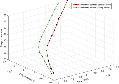
Further analysis, if penalty values of the qualitative factor are not added into the objective $f_{cost}$, Optimisation goals will only contain quantitative factors. The location results of each node quite differ from comprehensive optimisation, which shows in Table 10. As can be seen, the candidate A2 and A1 are selected at a higher ratio when only real costs are considered, which shows that they perform better in quantitative factors. Figure 6 shows the Pareto front for both. In each solution with the same responsiveness, the total costs and emissions are slightly higher than the results without penalty values, resulted from qualitative factors. It still changes location results (from A2 and A1 to A2 and A3), which demonstrates the effect of the comprehensive optimisation.

Table 10. The obtained Pareto solutions without penalty values.

	Objectives			Candidates
Node	fcost	fco2	fr	A1	A2	A3
1	13,491,290.3	780,492.3	26.4	33.33%	83.33%	0.00%
2	13,480,593.2	853,298.8	29.8	66.67%	83.33%	0.00%
3	13,476,296.5	889,785.8	31.5	83.33%	83.33%	0.00%
4	13,513,738.7	929,173.2	33.8	83.33%	100.00%	0.00%
5	13,606,754.5	993,422.4	36.1	83.33%	100.00%	33.33%
6	13,736,283.3	1,057,239.7	38.4	83.33%	100.00%	66.67%
7	14,397,352.5	1,137,638.8	40.8	100.00%	100.00%	83.33%
8	15,394,276.7	1,200,277.2	43.2	100.00%	100.00%	100.00%
9	16,549,846.9	1,245,066.4	45.6	100.00%	100.00%	100.00%
10	17,815,459.4	1,295,086.0	48.0	100.00%	100.00%	100.00%
11	19,157,551.1	1,348,761.5	50.4	100.00%	100.00%	100.00%
12	20,528,240.4	1,405,040.4	52.8	100.00%	100.00%	100.00%
13	22,030,400.2	1,463,747.2	55.2	100.00%	100.00%	100.00%
14	23,620,806.9	1,531,078.0	57.6	100.00%	100.00%	100.00%
15	25,366,235.5	1,597,711.6	60.0	100.00%	100.00%	100.00%
Average				88.89%	96.67%	65.56%

Figure 6. Comparison of two Pareto fronts.

5.3. Multi-scenario analyses

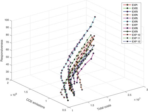
In the practical problem, demands, the return ratio, and the quality level are often uncertain. According to the distribution, each parameter can be divided into three different levels: lower bound (lb), mean, upper bound (ub). So, we designed nine experiments (EXP1-9) at different levels according to the orthogonal experimental method (L₉(3⁴)). The results will show the robustness of the location scheme under uncertainty. Meanwhile, we also designed three stochastic experiments (EXP10-12) for comparison, which will verify the conclusions of the orthogonal experiment. Table 11 contains the parameter value and results for each experiment. These 12 experiments represent different scenarios. For example, EXP1 indicates a scenario with medium level parameters, while EXP2 represents a scenario with the high return ratio but other parameters at the lowest level. Similarly, in each scenario, $\epsilon$ was also changed in 10% increment to get Pareto solutions and calculate the selection rate. Figure 7 contains the Pareto fronts for these different experiments. Combining EXP1-9, the final average selection rates of A2 and A3 exceed 85%, and the probability of selecting A1 is less than 35%. Therefore, the final location result can be considered as A2 and A3. The result is very robust because it has a high selection rate in most uncertain scenarios. EXP10-12 show similar rules, verifying the validity of this result. The average selection rate also shows that the order of priority of the collection centre is A3, A2, A1. This also indicates the sequence for opening collection centres.

Table 11. Optimal results in uncertain scenarios.

NO.	η	θ	λ	Demands	A1	A2	A3
Orthogonal experiments
EXP 1	0.35	0.3	0.5	mean	51.11%	96.67%	90.00%
EXP 2	0.35	0.25	0.4	lb	0.88%	83.33%	92.98%
EXP 3	0.35	0.35	0.6	ub	53.33%	100.00%	100.00%
EXP 4	0.2	0.3	0.4	ub	30.95%	67.86%	96.43%
EXP 5	0.2	0.25	0.6	mean	42.42%	71.21%	96.97%
EXP 6	0.2	0.35	0.5	lb	2.87%	68.97%	99.43%
EXP 7	0.5	0.3	0.6	lb	1.04%	98.96%	95.83%
EXP 8	0.5	0.25	0.5	ub	69.05%	100.00%	100.00%
EXP 9	0.5	0.35	0.4	mean	50.00%	100.00%	100.00%
Average					33.52%	87.44%	96.85%
Stochastic experiments
EXP 10	0.339	0.286	0.514	Uniform(lb, ub)	46.08%	96.08%	93.14%
EXP 11	0.269	0.262	0.535	Uniform(lb, ub)	40.35%	85.96%	90.35%
EXP 12	0.453	0.284	0.468	Uniform(lb, ub)	51.39%	100.00%	100.00%

Figure 7. Pareto fronts of different experiments.

Another analysis is about changing problem size, we test five different sizes of the logistics network. All problems require new penalty values calculated by FANP. After evaluating each site, we also used the proposed model and orthogonal experiments to solve these problems. Table 12 contains the distribution of collection centres in average selection rate intervals for each problem. It turns out that most collection centres must be opened. Especially in problems #3 and #5, since the scenario of EXP8 shows the highest level of demand and return ratio, the returned product exceeds the total capacity of all candidate collection centres, indicating that more collection centres need to be opened.

Table 12. Optimal results for different problem sizes.

	Problem size									Number of collection centres
No	i	j	k	l	m	n	d	Variables	Constraints	(85%,100%]	(75%,85%]	(65%,75%]	[0,65%]
#1	5	4	5	7	4	3	3	1170	1664	3	0	0	1
#2	7	6	7	11	5	4	4	2316	3014	3	1	1	0
#3	9	7	9	14	7	5	5	3738	4628	5	1	1	0
#4	13	10	14	19	9	7	6	7374	8612	6	1	1	1
#5	18	14	20	26	11	9	7	13,494	15,158	8	2	1	0

The results of the computational experiment provide the following significant conclusions:

When considering penalty values, the total costs do not increase significantly, because the influence of qualitative factors only occurs in the collection centre.

The orthogonality experiment can prove the robustness of location results, identify the priority of candidate sites, and can be extended to different scale problems.

6. Conclusion

Based on the general CLSC network structure, this paper designs a collection centre location model. It has positive significance to the establishment of reverse logistics in the whole supply chain. To assist the decision-makers to judge, this paper considers various factors. In the qualitative factors, this paper considers a total of 10 factors in three aspects of society, politics, and environment. All costs, $C{O}_2$ emissions, and responsiveness are also considered in quantitative factors. In order to synthesise all the factors, this paper proposes a novel approach which integrates FANP and MOMILP to analyse qualitative and quantitative factors. In the process of solving, FANP is used to evaluate 10 qualitative factors, and the evaluation value will be converted to the penalty coefficient to calculate the new fixed costs and relevant transportation costs. Then, they will be taken into the MOMILP to search the final results. This approach is proved to be effective in calculating the impact of qualitative factors. Meanwhile, this paper has depth analyses of uncertainty scenarios, orthogonal experiments are used to prove the robustness of the results. In the future, the framework can be appropriately expanded to take into account the cyclical effect of qualitative factors and consider multiple layers of location.

Disclosure statement

No potential conflict of interest was reported by the authors.

Additional information

Notes on contributors

Chuanrui Yang

Chuanrui Yang has received his bachelor's degree in logistics engineering and a master's degree in industrial engineering from Chongqing University. His main research areas are logistics and supply chain management.

Xiaohui Chen

Xiaohui Chen is a professor at the college of Mechanical Engineering at Chongqing University. Her main research areas  are logistics and supply chain management, modern enterprise management technology, and equipment reliability management.

References

- Alimoradi, A., R. M. Yussuf, N. B. Ismail, and N. Zulkifli. 2015. “Developing a Fuzzy Linear Programming Model for Locating Recovery Facility in a Closed Loop Supply Chain.” International Journal of Sustainable Engineering 8 (2): 122–137. doi:10.1080/19397038.2014.906514.
- Alimoradi, A., R. M. Yussuf, and N. Zulkifli. 2011. “A Hybrid Model for Remanufacturing Facility Location Problem in A Closed-Loop Supply Chain.” International Journal of Sustainable Engineering 4 (1): 16–23. doi:10.1080/19397038.2010.533793.
- Chan, F. T. S., N. Kumar, M. K. Tiwari, H. C. W. Lau, and K. L. Choy. 2008. “Global Supplier Selection: A fuzzy-AHP Approach.” International Journal of Production Research 46 (14): 3825–3857. doi:10.1080/00207540600787200.
- Cheng, S., C. W. Chan, and G. H. Huang. 2003. “An Integrated Multi-criteria Decision Analysis and Inexact Mixed Integer Linear Programming Approach for Solid Waste Management.” Engineering Applications of Artificial Intelligence 16 (5–6): 543–554. doi:10.1016/S0952-1976(03)00069-1.
- Ebrahimi, S. B. 2018. “A Stochastic Multi-objective Location-allocation-routing Problem for Tire Supply Chain considering Sustainability Aspects and Quantity Discounts.” Journal of Cleaner Production 198: 704–720. doi:10.1016/j.jclepro.2018.07.059.
- Govindan, K., H. Soleimani, and D. Kannan. 2015. “Reverse Logistics and Closed-Loop Supply Chain: A Comprehensive Review to Explore the Future.” European Journal of Operational Research 240 (3): 603–626. doi:10.1016/j.ejor.2014.07.012.
- Govindan, K. P., C. Jha, and K. Garg. 2016. “Product Recovery Optimization in Closed-Loop Supply Chain to Improve Sustainability in Manufacturing.” International Journal of Production Research 54 (5): 1463–1486. doi:10.1080/00207543.2015.1083625.
- Jatuphatwarodom, N., D. F. Jones, and D. Ouelhadj. 2018. “A Mixed-Model Multi-objective Analysis of Strategic Supply Chain Decision Support in the Thai Silk Industry.” Annals of Operations Research 267 (1–2): 221–247. doi:10.1007/s10479-018-2774-6.
- Kabir, G., and R. S. Sumi. 2014. “Power Substation Location Selection Using Fuzzy Analytic Hierarchy Process and PROMETHEE: A Case Study from Bangladesh.” Energy 72: 717–730. doi:10.1016/j.energy.2014.05.098.
- Kayikci, Y. 2010. “A Conceptual Model for Intermodal Freight Logistics Centre Location Decisions.” In 6th International Conference on City Logistics, edited by E. Tanguchi and R. G. Thompson, 6297–6311, Puerto Vallarta, Mexico, June 30-July 2. doi:10.1016/j.sbspro.2010.04.039
- Kuo, M.-S. 2011. “Optimal Location Selection for an International Distribution Center by Using a New Hybrid Method.” Expert Systems with Applications 38 (6): 7208–7221. doi:10.1016/j.eswa.2010.12.002.
- Melo, M. T., S. Nickel, and F. Saldanha-da-Gama. 2009. “Facility Location and Supply Chain Management – A Review.” European Journal of Operational Research 196 (2): 401–412. doi:10.1016/j.ejor.2008.05.007.
- Nagurney, A., and L. S. Nagurney. 2010. “Sustainable Supply Chain Network Design: A Multicriteria Perspective.” International Journal of Sustainable Engineering 3 (3): 189–197. doi:10.1080/19397038.2010.491562.
- Niroomand, S., A. Bazyar, M. Alborzi, H. Miami, and A. Mahmoodirad. 2018. “A Hybrid Approach for Multi-criteria Emergency Center Location Problem Considering Existing Emergency Centers with Interval Type Data: A Case Study.” Journal of Ambient Intelligence and Humanized Computing 9 (6): 1999–2008. doi:10.1007/s12652-018-0804-5.
- Özceylan, E., and T. Paksoy. 2013. “A Mixed Integer Programming Model for A Closed-loop Supply-Chain Network.” International Journal of Production Research 51 (3): 718–734. doi:10.1080/00207543.2012.661090.
- Ozgen, D., and B. Gulsun. 2014. “Combining Possibilistic Linear Programming and Fuzzy AHP for Solving the Multi-objective Capacitated Multi-facility Location Problem.” Information Sciences 268: 185–201. doi:10.1016/j.ins.2014.01.024.
- Pishvaee, M. S., R. Z. Farahani, and W. Dullaert. 2010. “A Memetic Algorithm for Bi-Objective Integrated Forward/Reverse Logistics Network Design.” Computers & Operations Research 37 (6): 1100–1112. doi:10.1016/j.cor.2009.09.018.
- Pishvaee, M. S., and J. Razmi. 2012. “Environmental Supply Chain Network Design Using Multi-Objective Fuzzy Mathematical Programming.” Applied Mathematical Modelling 36 (8): 3433–3446. doi:10.1016/j.apm.2011.10.007.
- Ramezani, M., M. Bashiri, and R. Tavakkoli-Moghaddam. 2013. “A New Multi-Objective Stochastic Model for A Forward/Reverse Logistic Network Design with Responsiveness and Quality Level.” Applied Mathematical Modelling 37 (1–2): 328–344. doi:10.1016/j.apm.2012.02.032.
- Roh, S. Y., H. M. Jang, and C. H. Han. 2013. “Warehouse Location Decision Factors in Humanitarian Relief Logistics.” Asian Journal of Shipping & Logistics. doi:10.1016/j.ajsl.2013.05.006.
- Tabari, M., A. Kaboli, M. B. Aryanezhad, K. Shahanaghi, and A. Siadat. 2008. “A New Method for Location Selection: A Hybrid Analysis.” Applied Mathematics and Computation 206 (2): 598–606. doi:10.1016/j.amc.2008.05.111.
- Temur, G. T. 2016. “A Novel Multi Attribute Decision Making Approach for Location Decision under High Uncertainty.” Applied Soft Computing 40: 674–682. doi:10.1016/j.asoc.2015.12.027.