Modelling and an improved NSGA-II algorithm for sustainable manufacturing systems with energy conservation under environmental uncertainties: a case study

ABSTRACT

This study addresses a flexible job shop scheduling problem considering the energy tax regulations. We introduce two strategies as reactive scheduling to deal with two different kinds of uncertainty. The first uncertainty is about the start and processing times of the jobs with a known probability distribution. The second kind is related to machine breakdowns, modification or cancellation of the orders, and receive new orders without any known probability distribution. Two conflict objective functions are considered as minimising tax cost on surplus energy consumption and minimising total cost of jobs lateness based on soft time-windows. A bi-objective mathematical model is developed to formulate the problem. Since the problem is well-known strongly NP-hard, a new solution approach is introduced based on the NSGA-II algorithm to solve the problem in a reasonable computational time. Some test problems based on a real case study are used to evaluate the performance of the proposed solution approach. The result analysis confirms the effectiveness of the proposed algorithm and its superiority comparing with another algorithm based on the classic NSGA-II. Moreover, sensitivity analysis is done on the main parameters to provide proper managerial suggestions based on the obtained Pareto front solutions.

KEYWORDS:

• Flexible job shop
• reactive scheduling
• energy-saving
• floating scheduling operator
• soft time-windows

1. Introduction

Nowadays, all countries in the world are facing a serious challenge such as the energy crisis and environmental pollution. To tackle this common world threat, many efforts have been done on broadening the sources of energy and reducing the consumption/cost of energy (Yang et al. 2020). According to a report of the International Energy Agency (IEA), demand for energy consumption in the world will increase by 35% in the upcoming 15 years (Tang, Warkentin, and Wu 2019). Due to the limited available energy resources, energy-saving is very important and vital for all countries in the world to achieve sustainable economic growth in all sectors (Cai et al. 2019; Long et al. 2018). Given that the manufacturing industry is the most important sector in the development of the economy. For this reason, more than 40% of the world’s energy consumption is allocated to them (Danielle et al. 2011; Bruzzone et al. 2012; Duflou et al. 2012; Li and Lin 2016). According to the opinion of economists, governments are on the economic growth that has put the tax on energy consumption (van Zon and Yetkiner 2003). Governments of developed countries have implemented tax regulations to prevent greenhouse gas emissions and to ensure more energy-saving. Manufacturing industries affected by government energy-saving regulations must pay very high taxes on surplus energy consumption. Therefore, these policies impose many restrictions on many manufacturing industries to reduce energy consumption via optimisation of production scheduling. The make-to-order (MTO) systems based on casting and multi-machine scheduling are a type of these manufacturing industries that almost uses high-powered machines and technology such as induction melting furnaces. In the nowadays-competitive environment, such industries are usually facing some challenges such as high penalty costs of lateness in delivering orders and high tax costs on surplus energy consumption to governments. It is especially vital for managers to minimise these costs and to make a trade-off between these conflict objectives under uncertainty.

Job shop scheduling is one of the most popular scheduling problems in the MTO system. Unexpected disruptions during running original predictive scheduling lead to failure in original scheduling. Such industries are forced to pay very high production costs for facing minor disruptions in the original scheduling because of their higher lateness penalties comparing to other industries. Moreover, machines of such industries use more energy. Therefore, uncertainties during running original predictive scheduling lead to increase costs of energy consumption.

Consequently, in previous years, researchers have found that flexible job shop scheduling (FJSS) can be an efficient method for overcoming the existing uncertainty (Gao, Gen, and Sun 2006; Gao et al. 2007; Gao, Sun, and Gen 2008; Gen, Gao, and Lin 2009). Studies of such industries have shown that uncertainty is caused by factors such as job inaccessibility, inadequate estimation of processing time, machine breakdowns, modifications of the orders, and receive new orders (Herroelen and Leus 2005).

In this paper, two types of uncertainties are investigated for the FJSS problem with the nature of casting that almost uses high-powered machines. The first type includes the uncertainties with pre-known probability distribution such as inaccessibility of resources and jobs. Such uncertainties may lead to the creation of stochastic parameters and variables especially in the operations start time of jobs. Moreover, uncertainties such as lack of skilled manpower and inadequate estimation of processing time may lead to the creation of stochastic parameters in the operations processing time of jobs. For these parameters, we need to define a probability distribution to present the proper stochastic scheduling (Kall and Wallace 1994). For this reason, in the presented mathematical model of this study, the start and processing time of operations are considered as stochastic parameters with a uniform probability distribution.

The second type of uncertainties includes parameters that follow no well-known probability distribution such as machine breakdowns and modification or cancellation of the orders, changing of the delivery dates, and receiving new important orders. Such uncertainties that occur as unexpected disturbances during running original predictive scheduling may lead to failure in initial scheduling. For this purpose, reactive scheduling will be used to deal with these types of disruptions.

To optimise solutions in the face of unexpected events, the best way is to use reactive scheduling and this type of scheduling method is provided as a revised version of real-time scheduling. In the other words, most pre-scheduling activities in real-time scheduling can be defined better through reactive scheduling. Reactive scheduling is divided into two categories (Herroelen and Leus 2004): the first category is rescheduling, and the second is scheduling repair. In this paper, we use scheduling repair for responding to disruptions during running the original predictive scheduling. Scheduling repair would be a proper approach to adapt the original scheduling to the new status. This approach attempts to improve the original scheduling so that the best results are achieved in terms of unexpected internal and external disruptions. The best reactive strategies for responding to disruptions are in two ways. Firstly, the system can allocate multiple machines into each operation of jobs, and secondly, the system is able to select the best alternative process for other jobs.

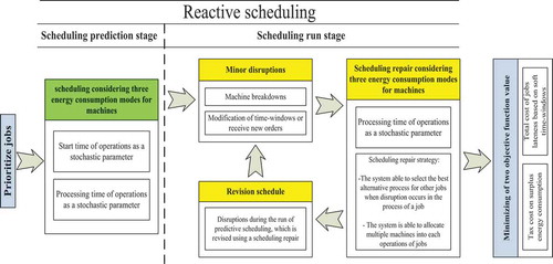
As stated above, this paper provides an appropriate approach to respond to two general types of uncertainties in a stochastic flexible job shop scheduling (SFJSS) problem. Stochastic scheduling is used for responding appropriately to the uncertainties of the first type such as start and processing stochastic time with a uniform probability distribution. Reactive scheduling is used for dealing with the second type of uncertainties such as machine breakdowns and modification or cancellation of the orders, changing of the delivery dates, and receiving important new orders, appropriately. Energy consumption in switching machine modes has considered adjusting the machine’s status in two of the three modes such as processing, idle, and standby. For this purpose, we aim to minimise tax cost on surplus energy consumption and total cost of jobs lateness based on soft time-windows using scheduling repair in the original predictive scheduling, which is failure due to the effect of unexpected disruptions.

The conceptual model of reactive scheduling for disruptions in SFJSS with energy-saving regulations has been shown in Figure 1.

Figure 1. A schematic view of the proposed approach in this research

In general, this study attempts to answer the following research question: ‘How can industry owners do to a trade-off between total costs of jobs lateness based on soft time-windows and tax cost on surplus energy consumption with uncertain parameters?’. To better present the place of the main features of this study among previous studies, a comparison has been made in five different aspects.

1.1. Related studies in energy-saving

Studies in this field can be divided into four groups including energy- saving using the turn on/turn off approach, the speed level adjustment approach, peak consumption, and government regulations. In the first group, researchers have used the turn on/turn off approach considering a pre-defined amount for the idle mode to minimise total energy consumption. Researchers proposed a single-machine scheduling problem using a neural network to determine the status of turn-off or idle modes in the time gap between two jobs (Mouzon, Yildirim, and Twomey 2007). In 2008, researchers introduced a concept called break-even which is a criterion for determining the turn-off or idle state of the machine (Mouzon and Yildirim 2008). Also, the control coefficient of the turn-off machine was provided for the flow shop scheduling problem (Dai et al. 2013). Also, other researchers considered energy consumption as an objective function with the possibility of the turn off the machine to energy-saving in single-machine scheduling problems (Che et al. 2017). Wu & Sun employed both of the turn on/turn off approach and different speeds for processing to minimise the energy consumption and makespan in a flexible job shop scheduling problem simultaneously (Wu and Sun 2018).

In the second group, researchers have tried to minimise total energy consumption using the speed level adjustment approach without affecting the makespan. Then, studies were conducted on two machines with different speeds for flow shop scheduling problems (Mansouri, Aktas, and Besikci 2016). Even in 2015, researchers studied the energy consumption of machines in idle and processing modes for the dynamic flow shop scheduling problem when the new job arrival and machine breakdown were under consideration (Dai 2015). In the same group, some researchers proposed a teaching-learning-based optimisation (TLBO) to solve the hybrid flow shop scheduling problem which is made up of three subproblems including scheduling, machine assignment, and speed selection (Lei, Gao, and Zheng 2017). Similarly, Chen et al. employed a collaborative optimisation algorithm to minimise makespan and total energy consumption simultaneously, in which a speed adjusting strategy for the non-critical operations is designed to improve total energy consumption (Chen, Wang, and Peng 2019). Due to the notable influence of the speed change approach on energy-saving, this issue receiving increasing attention in the field of academic during last years (Zhang and Chiong 2016; Fu et al. 2019; Li, Lei, and Cai 2019; Luo, Zhang, and Fan 2019; Wu and Che 2020).

In the third group, some approaches for energy-saving in peak consumption have been considered. In this type of scheduling, attempts have been made to shift operations of jobs to off-peak times to reduced energy consumption. The turn off of machines at the off-peak in flexible production systems was investigated for energy-saving (Pach et al. 2014). In the same year, researchers investigated the same problem in which energy prices were multiple at different times and this approach was applied to a single machine scheduling problem (Shrouf et al. 2014). Also, a bi-objective mixed integer programming mathematical model was proposed by researchers at different energy prices in the single machine batch scheduling problem (Cheng et al. 2017). As a new study, researchers tackled the scheduling problems under Time-of-Use (TOU) tariffs to minimise the total power cost by appropriately scheduling the jobs in a way that the overall completion time not be exceeded from a predetermined production deadline (Cheng, Chu, and Zhou 2018).

In the fourth group, researchers applied different energy-saving approaches based on government regulations such as subsidies and tax rules. The effect of the energy-saving approach has been analysed by implementing various subsidy regulations (preferential tax, price subsidy, sales, and investment subsidy) on the amount of production and profit (Zhang et al. 2014). Two competitive supply chains were investigated by researchers. Thus, they analysed four competitive combinations of the supply chain with four government sub-objectives function (energy-saving, net income, social welfare, and sustainable development) (Hafezalkotob 2017).

In general, compared with the four aforementioned groups, it can be concluded that machines in the MTO systems especially based on casting are rarely turned off but the amount of energy consumption in switching the idle and standby modes of machines is significant. Furthermore, the cost of government taxes on surplus energy consumption in such manufacturing industries is notable. It is also notable that, a few researchers have investigated the energy consumption issue considering machine switching in flexible job shop scheduling problems under government tax regulations. Therefore, this issue is the first main feature studied in this paper.

1.2. Related studies in reactive scheduling

Unexpected disruptions during production that do not follow a certain probability distribution lead to failure in the original predictive scheduling and reactive scheduling is the best approach to reconsider in the original predictive scheduling. Researchers have considered a reactive scheduling problem in a stochastic environment. They analysed several scheduling policies in the conditions of machines’ inaccessibility for a classic job shop system (Sabuncuoglu and Bayiz 2000). One year later, the researchers proposed a reaction scheduling problem with the simultaneous application of average job’s tardiness and average job’s cost (Chryssolouris and Subramaniam 2001). Then, reactive job shop policies were considered in the condition of lack of access to machines and It was also suggested that time be revised based on a concept of control limits (Suwa and Sandoh 2007). In 2008, a reactive flexible job shop scheduling problem was considered for optimisation of lead time (Wu 2008). An event-oriented policy was considered to be reactive to the scheduling of the job shop with the stochastic arrival of jobs with machines inaccessibility. They also measured the performance of a multi-objective function, including tardiness of jobs and makespan (Adibi et al., 2010).

It can be concluded based on the previous studies that, a few researchers have conducted reactive scheduling problems considering machine breakdowns, changing the delivery dates, and conducting a new order based on a mathematical model. Therefore, this issue is the second main feature that is studied in this paper.

1.3. Related studies in stochastic scheduling

Stochastic scheduling is used to schedule jobs under the uncertainties that occur during production and follow a pre-known probability distribution. A flexible job shop scheduling problem was conducted under uncertainty and dynamic jobs arriving as well as sequences-dependent setup time of machines and some dispatch rules were introduced that are typically incorporated into two new methods in a simulated model (Kianfar, Fatemi Ghomi, and Oroojlooy Jadid 2012). Then, researchers solved the problem of dynamic flow shop scheduling when new jobs have arrived and machines are not available (Dai 2015).

The above studies have shown that four fields are usually considered for stochastic scheduling in flow shop and job shop such as starting time (Inaccessibility to machines or jobs), processing time (changes in time, special changes), machine breakdowns, and urgent jobs. In this paper, both of two approaches i.e., reactive scheduling and stochastic scheduling are considered in this study to investigate as a mathematical model for job shop scheduling problems. Therefore, this issue is one of the unique features studied in this paper.

1.4. Related studies considering similar objective functions

Creating a balance between different objectives is the inevitable challenge for the MTO systems. This paper aims to optimise two important conflict objective functions include the tax cost on surplus energy consumption and total cost of jobs lateness simultaneously. Such objective functions in flexible job shop scheduling problems have less attention paid by researchers. Mouzon proposed a model to minimise total energy consumption and delay for single machines (Mouzon and Yildirim 2008). A paper published in 2015 looked at minimising energy consumption with a maximum of limited tardiness in a single-machine problem (Che et al. 2015). Zhang et al. proposed a model to minimise the total tardiness and the energy consumption for a flexible job shop scheduling problem (Zhang and Chiong 2016). As another instance, Luo et al. developed a new decoding method and two Pareto-based mechanisms to obtain active schedules for a flexible job shop considering two aforementioned objectives (Luo, Zhang, and Fan 2019). Recently, researchers investigated the FJSS problem to minimise the makespan and the total energy consumption simultaneously while the total tardiness has been considered as a constraint. In this work, the authors used a chance-constrain approach to describe decision-makers’ awareness of total tardiness (Fu et al. 2019).

1.5. Related studies considering the solution algorithms

Most GA-based developed solution algorithms are mainly constructed based on three operators of selection, crossover, and mutation in combination with other heuristic and meta-heuristic algorithms. Studies were conducted in 2010 to minimise the maximum fuzzy completion time based on an efficient decomposed-integration GA (Lei 2010). A genetic algorithm was designed for strategic scheduling of cycle-driven in the case of a flexible job shop dynamic scheduling (Liu et al. 2011). A genetic simulated annealing algorithm was introduced in the flexible flow shop scheduling problem (Dai et al. 2013). In 2015, to manage the release time, the researchers looked at two meta-heuristic algorithms such as GA and PSO (Rey et al. 2015). A hybrid genetic algorithm integrating the local search was proposed to minimise the total tardiness and energy consumption (Zhang and Chiong 2016). In later years, researchers established a model to compute the energy consumption of machine tools at different machining stages and developed a green scheduling heuristic method to optimise makespan (He et al. 2015). Thereinafter, researchers used a hybrid GA and glow-worm swarm optimisation algorithm with a green transport heuristic strategy (GA-GSO-GTHS) (Liu, Guo, and Wang 2019). For the multi-objective flexible job-shop scheduling problems, the authors considered the transportation constraints and proposed an enhanced genetic algorithm to solve the multi-objective optimisation model with energy consumption and makespan (Dai et al. 2019). Meanwhile, researchers proposed a bi-objective ant colony optimisation to minimise the total energy consumption and makespan for an energy-aware batch scheduling problem (Jia et al. 2019).

Due to the bi-objective problem of this paper, the NSGA-II has been used in the development of the algorithm based on GA. In the proposed algorithm, another new operator called the ‘Floating Operator’ is utilised in addition to classic operators which may have many applications, especially in stochastic scheduling and reactive scheduling. In general, the studies conducted in the five fields mentioned can be shown in Figure 2.

Figure 2. A framework of fields studied in this research

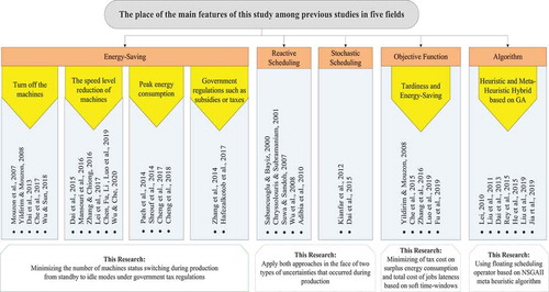
In summary, the majority of the scheduling problems in the energy-saving field are investigated in a single machine environment for each processing stage. However, there is usually more than one machine as parallel in some critical processing stages to increase flexibility such as the FJSS problem and less work has been done on such multi-machine problems. In such cases, no study has applied reactive scheduling and stochastic scheduling simultaneously to tackle both of the two main types of uncertainties. Furthermore, in the previous studies, less attention has been paid to two conflicting objectives include minimising tax cost on surplus energy consumption and minimising the total cost of jobs lateness based on a soft time-windows. Therefore, this study aims to minimise these two objective functions in a flexible job shop scheduling problem with a soft time-windows for a due date under uncertainty and a casting factory is studied as a real-world case study. In this way, a new mathematical model is introduced that can solve the problem with small dimensions, and a meta-heuristic algorithms based on a non-dominated sorting approach are developed to solve the large-sized instances in a reasonable time. So, we can summarise the contributions of this study in three categories as below:

Deciding on the best state of energy consumption in switching machine modes to reduce the costs imposed by government tax regulations: We usually have a high amount of energy dissipation in switching the modes of machines used in MTO systems based on casting. This is because of high-powered machines have been used such as induction melting furnaces. Increasing the number of machines status switching during production from standby to idle modes dramatically increases energy consumption. In such cases, tax costs on surplus energy consumption imposed on industry owners. Therefore, a new model is introduced to minimise tax costs on surplus energy consumption by adjusting machines on the best mode.

Introducing a new mathematical model for simultaneous use of reactive scheduling and stochastic scheduling approaches to reduce costs arising from government tax regulations and lateness based on delivery soft time-windows: Jobs scheduling in a flexible job shop problem is very difficult when industry owners are facing some known and unknown uncertainties during production. Applying the two approaches of reactive scheduling and stochastic scheduling to deal with each of the uncertainties in the framework of an exact mathematical model is one of the main features of the study in this research. It should be explained that few studies in this area have just proposed simulation approaches without any exact model. The proposed model in this study can provide the optimum solution with the minimum tax cost on surplus energy consumption and total cost of jobs lateness based on soft time-windows whenever any disruption has happened.

Using floating scheduling operator based on NSGA-II meta-heuristic algorithm: Given that the floating operator is applied to the body of the sub chromosome, it allows the algorithm to perform the best local search in the local feasible spaces. In other words, the operator allows operations of the job to be floating within a certain range and find the best value of objective functions in local feasible spaces. This algorithm has been developed based on NSGA-II, which uses three operators including selection, crossover, and mutation to find the feasible spaces and the best local search can be done in the same space using the floating operator.

The remaining sections of this paper are organised as follows: the problem is described in the form of a case study in section 2. In section 3, the mathematical model is presented. The solution approach is presented in section 4. Then, the proposed model is investigated using data from a real case study in a factory with a casting process. In the following, computational result and sensitivity analysis is presented in section 5. Finally, the paper is concluded with different dimensions of the problem in section 6 as the last section.

2. Problem description in the form of a case study

Reactive flexible job shop scheduling problem with energy-saving in a stochastic environment can be described as follows: There are $B$ jobs to do in this problem and the $w$^th job consists of a maximum of $N_w$ operations, which are processed using the $M_l$ parallel machines in the$l$^th stage. Parallel machines consume the same amount of energy at each stage in three statuses: processing mode, idle mode, and standby mode. In addition, the parallel machines have the same speed level. The machines never turn off due to the high cost of restarting. Therefore, the machines between the two consecutive operations are only in two statuses of idle mode or standby mode. It is worth mentioning that the machines in each stage use a certain amount of energy to status switching from standby to idle modes and on the contrary. The machine keeps in idle mode when the energy consumption between two consecutive operations in the idle mode is less than the required energy for switching from standby to idle mode. Otherwise, it is wise to machine adjust in standby mode to reduce energy consumption. Each operation of each job is assigned just to one machine in needed stages. The operations sequence of a job has already have been specified and cannot be changed. Start time and processing time are considered stochastic with a uniform probability distribution. There are two types of disruption during production including machine breakdowns and modification or cancellation of the orders, changing of the delivery time-windows, and receiving important new orders.

The first task of this problem is to create the best allocation of machines to operations by observing the priority of operations on the machine and the sequence of operations on the jobs. For this purpose, jobs should be delivered to the customers in the least possible deviation from the soft time-windows even in an uncertain environment. The second task of this problem is to decide about the best adjustment of the machine’s status switching between two consecutive operations to reduce energy consumption within the framework of government regulations. This problem is conducted in this study considering two conflict objective functions as total costs of jobs lateness based on soft time-windows and tax cost on surplus energy consumption.

The main features of this problem are defined with inspiration from a casting industry as a real case study. The considered casting factory manufactures a variety of parts for the automotive industries as an MTO system using different processes including induction melting furnace, machining, milling, and sandblast. In the B16 department of this factory, ball bearing parts are custom manufacturing and repairing for all types of automobiles. The factory has seven machines in total in which, the casting stage has two parallel machines with different energy consumption and after that there is the machining stage with three parallel machines with different energy consumption. Furthermore, there is one machine for each of the millings and sandblast stages. In the first half of August 2019, this factory received orders to build three parts and repair two parts in the ball bearing sector.

A contract has been concluded with the customers, who the orders will be delivered in a soft time-windows according to the Table 1. The contract concluded by the department of commerce provides penalties for job lateness outside the time-windows. In Table 1, the upper bound and the lower bound of the delivery time window of the $w$^th job have been presented as $d{u}_w^{\tau }$ and $d{l}_w^{\tau }$ respectively in the original scheduling $\left(\tau \right)$. Also, the items $V{E}_w$ and $V{L}_w$indicate the amount of penalty for delivery earlier and later than the specified time window of $w$^th job respectively.

Table 1. Delivery time-windows and lateness penalty of the jobs based on original scheduling ($\tau$)

Jobs	1	2	3	4	5
$d{u}_w^{\tau }$	21	41	19	35	45
$d{l}_w^{\tau }$	18	39	15	30	41
$V{L}_w$	140	300	350	180	90
$V{E}_w$	100	200	250	140	50

For example, as is evident in this table, there is a 140$ penalty per hour for the lateness in delivery the job 1. While delivering this product earlier than the specified lower bound in the time-window (18) will impose 100$ per hour. The production planning department is going to a proper schedule with a minimum of total tax cost on surplus energy consumption and total cost of jobs lateness based on soft time-windows per hour. The real-time occurrence of the original predictive scheduling is shown in Table 2 based on the scheduling of the Company’s production planning department. The start time and the processing time are determined as stochastic (with uniform distribution). According to Table 2, the operation 1 of the first job is assigned to ${\mathrm{M}}_{11}$, which means the first machine in the first stage. The process starts at 1 o’clock randomly, and the processing time takes 5 hours randomly. In addition, the operation process takes 10 hours after breakdowns and repairing the machine.

Table 2. The real-time occurrence of the original predictive scheduling (Start and processing stochastic time)

	Operation 1		Operation 2		Operation 3		Operation 4
Job 1	M11	1;5,10	M41	8;4,9	M21	16;4,4		-
Job 2	M32	3;5,5	M11	8;6,13	M41	20;11,13	M22	33;9,8
Job 3	M23	2;11,14	M41	13;5,9	-
Job 4	M31	4;12,7	M11	16;7,7	M22	48;11,12	M41	66;6,4
Job 5	M41	2;6,12	M11	28;8,9	M23	38;5,3

The power consumption of the machines at each stage in three modes such as processing, idle, and standby as well as the power consumption of each machine to switch from standby to idle modes based on the energy label of the machines in kw/h are illustrated in Table 3. In Table 3, the item $H_{lm}$ shows the power consumption of the $m$^th machine in the $l$^h stage for switching from standby to idle mode.

Table 3. Machine parameters in energy consumption (kw/h)

$M_{lm}$	Processing Power	Idle Power	Standby Power	$H_{lm}$
$M_{41}$	1220	953	20	5000
$M_{32}$	3120	2950	120	6123
$M_{31}$	3120	2950	120	6123
$M_{23}$	1500	1205	52	3421
$M_{22}$	1500	1205	52	3421
$M_{21}$	1500	1205	52	3421
$M_{11}$	2532	2102	80	5345

For example, it can be found from this table that the power consumption of machine 1 in the fourth stage (M41) is 1220 kw/h, 953 kw/h, and 20 kw/h in the processing mode, idle mode, and the standby mode respectively. In addition, the power consumption of the mentioned machine is equivalent to 5,000 kw/h for switching from standby to idle modes. According to calculations based on government tax regulations, the maximum amount of power consumption is 200,000 kw/h for producing the five aforementioned parts and surplus energy consumption causes a tax cost of 3000$ per hour. However, two kinds of disruptions happen at 10 o’clock during the real-time occurrence of the original predictive scheduling. The first disruption happened because some preventive maintenance modifications were not implemented on some machines; the machines are damaged and are out of the production circuit for a certain period. The inaccessibility time of each machine based on the first disruption is shown in Table 4.

Table 4. Duration of inaccessibility on machines in each stage ($I_{lm}^{\gamma }$)

$\left[\underset{m}{\overset{l}{\hspace{0.17em}}}\right]$	1	2	3	4
1	3	0	0	5
2	0	2	0	0
3	0	5	0	0

The second disruption is that the customers called and asked the factory to change the delivery time window in lieu of paying the factory according to Table 5. In Table 5, the items $d{u}_w^{\mathit{\gamma }}$ and $d{l}_w^{\mathit{\gamma }}$ show the upper bound and the lower bound of the delivery time window for the $w$^th job in the reactive scheduling $\left(\mathit{\gamma }\right)$, respectively.

Table 5. Delivery time-windows and lateness penalty of the jobs based on reactive scheduling ($\mathit{\gamma }$)

Jobs	1	2	3	4	5
$d{u}_w^{\mathit{\gamma }}$	16	35	17	28	41
$d{l}_w^{\mathit{\gamma }}$	14	33	15	25	40
$V{L}_w$	140	300	350	180	90
$V{E}_w$	100	200	250	140	50

In the next section, a new mathematical model is introduced to response to unexpected disruptions and uncertainties during production using strategies of scheduling repair and energy consumption in switching machine modes.

3. Mathematical model for reactive scheduling in SFJSS problem

In this section, a new mathematical model is proposed to deal with the two types of mentioned uncertainties during production. So, the model is proposed based on the repair strategy and stochastic scheduling approach. Meanwhile, minimising the total cost of jobs lateness as well as minimising the tax cost on surplus energy consumption is considered as two objectives. In the following, first, the main assumptions of the considered problem are presented and then, notations and mathematical model of the problem is introduced as a mixed-integer programming (MIP) model.

The operations sequence of a job has already been specified and cannot be changed

Each operation of each job is assigned just to one machine in needed stages.

Each machine can only process one operation of a job at a certain moment

Sequences of jobs on machines are prioritised.

Once start, the process cannot be interrupted.

Setup times are independent and considered as a section of processing time.

Start time and processing time are considered stochastic with a uniform probability distribution

Also, the following notations are used to formulate the considered problem:

Table

Indices
$w,t,a$	Indices for jobs, $w,t,a\in \left\{1,2,\dots ,B\right\}$
$o,p,r$	Indices for operations, $o,p,r\in \left\{1,2,\dots ,N_w\right\}$
$m$	Index for machines, $m\in \left\{1,2,\dots ,M_l\right\}$
$l$	Index for stages, $l\in \left\{1,2,\dots ,L\right\}$
General parameters
$B$	The number of total jobs.
$L$	The number of total stages.
$N_w$	The number of total operations for the $w$^th job.
$M_l$	The number of total parallel machines in the $l$^th stage.
$A_{wo}$	The $o$^th operation of the $w$^th job.
$F_{lm}$	The processing power of $m$^th machine in the $l$^th stage.
$V_{lm}$	The idle power of $m$^th machine in the $l$^th stage.
$S_{lm}$	The standby power of $m$^th machine in the $l$^th stage.
$H_{lm}$	The power of $m$^th machine in the $l$^h stage to switch from standby to idle mode.
${\beta }_{lwo}$	A binary parameter that takes value 1 if the $o$^th operation of the $w$^th job requires to the stage $l$^th; 0, otherwise.
$V{E}_w$	Penalty for delivery earlier than the specified time window of $w$^th job to the customer
$V{L}_w$	Penalty for delivery later than the specified time window of $w$^th job to the customer
$T$ R M	The tax rate on surplus energy consumption The maximum allowed for energy consumption according to thr government tax regulation. A large number.
Parameters for the original scheduling before disruptions $\left(\tau \right)$
$B^{\tau }$	The set of jobs in the original scheduling$\left(\tau \right)$.
$e{p}_{lwom}^{\tau }$	The earliest processing time of $A_{wo}$ on the $m$th machine in the $l$th stage in the original scheduling $\left(\tau \right)$ as deterministic.
$c{p}_{lwom}^{\tau }$	The latest processing time of $A_{wo}$ on the $m$th machine in the $l$th stage in the original scheduling $\left(\tau \right)$ as deterministic.
$\xi p_{lwom}^{\tau }$	Processing time of $A_{wo}$ on the $m$^th machine in the $l$^h stage in the $\left(e{p}_{lwom}^{\tau },c{p}_{lwom}^{\tau }\right)$ time-interval in the original scheduling $\left(\tau \right)$ as stochastic.
$d{u}_w^{\tau }$	Upper bound of delivery time window of $w$^th job in the original scheduling $\left(\tau \right)$.
$d{l}_w^{\tau }$	Lower bound of delivery time window of $w$^th job in the original scheduling $\left(\tau \right)$.
$e{t}_{wo}^{\tau }$	The earliest start time of $A_{wo}$ in the original scheduling $\left(\tau \right)$ as deterministic.
$c{t}_{wo}^{\tau }$	The latest start time of $A_{wo}$in the original scheduling $\left(\tau \right)$ as deterministic.
$\xi t_{wo}^{\tau }$	Start time of $A_{wo}$ in the ($e{t}_{wo}^{\tau },c{t}_{wo}^{\tau })$time-interval in the original scheduling$\left(\tau \right)$as stochastic.
$K^{\tau }$	Occurrence time of disruption in the original scheduling $\left(\tau \right)$.
${\phi }_{lwom}^{\tau }$	A binary parameter that takes value 1 if the $m^{th}$ machine is allocated to the $A_{wo}$in the $l^{th}$ stage in the original scheduling $\left(\tau \right)$; 0, otherwise.
$D_{wotp}^{\tau }$	Distance between $A_{wo}$and $A_{tp}$ in the original scheduling$\left(\tau \right)$
Parameters for the reactive scheduling after disruptions $\left(\gamma \right)$
$B^{\gamma }$	The set of corrected jobs in the reactive scheduling $\left(\gamma \right)$.
$e{p}_{lwom}^{\gamma }$	The earliest processing time of $A_{wo}$ on the $m^{th}$ machine in the $l^{th}$th stage in the reactive scheduling $\left(\gamma \right)$ as deterministic.
$c{p}_{lwom}^{\gamma }$	The latest processing time of $A_{wo}$ on the $m$th machine in the $l$th stage in the reactive scheduling $(\gamma )$ as deterministic.
$\xi p_{lwom}^{\gamma }$	Processing time of $A_{wo}$ on the $m$^th machine in the $l$^th stage in the $\left(e{p}_{lwom}^{\gamma },c{p}_{lwom}^{\gamma }\right)$ time-interval in the reactive scheduling $\left(\gamma \right)$ as stochastic.
$d{u}_w^{\gamma }$	Upper bound of corrected delivery time window of the $w$^th job in the reactive scheduling $\left(\gamma \right)$.
$d{l}_w^{\gamma }$	Lower bound of corrected delivery time window of the $w$^th job in the reactive scheduling $\left(\gamma \right)$.
$I_{lm}^{\gamma }$	Duration of inaccessibility to the $m$^th machine in the $l$^th stage in the reactive scheduling $\left(\gamma \right)$.
Decision variables
${\vartheta }_{wo}^{\tau }$	Binary variable takes value 1 if start time of $A_{wo}$ occurs sooner than disruption time in the original scheduling $\left(\tau \right)$; 0, otherwise.
${\psi }_{lwom}^{\gamma }$	Binary variable that takes value 1 if the $m$^th machine is allocated to the $A_{wo}$in the $l$^th stage in the reactive scheduling ($\gamma$); 0, otherwise.
$\xi t_{wo}^{\gamma }$	Start time for $A_{wo}$ in reactive scheduling $\left(\gamma \right)$ as stochastic.
${\delta }_{lwt}$	Binary variable taking value 1 if the$w$^th job is the precedence of the $t$^th job and both of them requires to be process in the$l$^th stage; 0, otherwise.
${\omega }_{wotp}$	Binary variable taking value 1 if the machine is idle mode between $A_{wo}$and $A_{tp}$; 0, otherwise.
${\nu }_{wo}$	Binary variable taking value 1 if the $A_{wo}$ is complete before disruption time in the original scheduling $\left(\tau \right)$; 0, otherwise.
${\zeta }_{wo}$	Binary variable taking value 1 if the $A_{wo}$is complete before disruption time and inaccessible to machine in the original scheduling $\left(\tau \right)$; 0, otherwise.
$G_{lwoartpm}$	Binary variable taking value 1 if $A_{ar}$ is between $A_{wo}$ and $A_{tp}$ and all three of them assign to the$m$^th machine in the $l$^th stage; 0, otherwise.
Objective functions
$Q$	Tax cost on surplus energy consumption.
$Y$	Total cost of jobs lateness based on soft time-windows.
$QTF{1}_{lmwotp}$	The distance between two successive operations $A_{wo}$ and $A_{tp}$ on the mth machine in the l^th stage in the original scheduling $\left(\tau \right)$.
$QTF{2}_{lmwotp}$	The distance between two successive operations $A_{wo}$ and $A_{tp}$ on the m^th machine in the l^th stage in reactive scheduling $\left(\gamma \right)$.
$QTF{3}_{lmwotp}$	The distance between two successive operations $A_{wo}$ and $A_{tp}$ on the m^th machine in the l^th stage while one of them is in the original scheduling $\left(\tau \right)$ and the other is in reactive scheduling $\left(\gamma \right)$.
$Q_{F_{\left(lm\right)}}$	The energy consumption of the $m$^th machine in the$l$^th stage in the processing mode.
$Q_{V_{\left(lm\right)}}$	The energy consumption of the $m$^th machine in the $l$^th stage in the idle mode.
$Q_{V_{\left(lmwotp\right)}}$	The distance between two successive operations Awo and Atp on the m^th machine in the l^th stage in the idle mode.
$Q_{S_{\left(lm\right)}}$	The energy consumption of the $m$^th machine in the $l$^th stage in the standby mode.
$Q_{S_{\left(lmwotp\right)}}$	The distance between two successive operations Awo and Atp on the m^th machine in the l^th stage in the standby mode.

The proposed mathematical model

(1) $\begin{array}{rl}& Y=\\ & =\sum _{w=1}^{B}max\left(\begin{array}{c}0,((\xi t_{w{N}_w}^{\gamma }+\sum _{l=1}^L\sum _{m=1}^{M_l}\xi p_{lw{N}_{w}m}^{\gamma }.{\psi }_{lw{N}_{w}m}^{\gamma })-d{u}_w^{\gamma }).V{L}_w\end{array}\right)\\ & +max\left(0,(d{l}_w^{\gamma }-\left(\xi t_{w{N}_w}^{\gamma }+\sum _{l=1}^L\sum _{m=1}^{M_l}\xi p_{lw{N}_{w}m}^{\gamma }.{\psi }_{lw{N}_{w}m}^{\gamma })\right).V{E}_w\right)\end{array}$(1)

(2) $Q=max\left(0,\left(\sum _{l=1}^L\sum _{m=1}^{M_l}{Q}_{F_{\left(lm\right)}}+\sum _{l=1}^L\sum _{m=1}^{M_l}{Q}_{V_{\left(lm\right)}}+\sum _{l=1}^L\sum _{m=1}^{M_l}{Q}_{S_{\left(lm\right)}}-R\right).T\right)$(2)

(3) $Q_{F_{\left(lm\right)}}=F_{lm}.\left(\sum _{w=1}^B\sum _{o=1}^{N_w}\xi p_{lwom}^{\gamma }.{\psi }_{lwom}^{\gamma }+\xi p_{lwom}^{\tau }.{\phi }_{lwom}^{\tau }.{\vartheta }_{wo}^{\tau }\right),\mathrm{\forall }l,m$(3)

(4) $Q_{V_{\left(lm\right)}}=V_{lm}.\sum _{w=1}^B\sum _{o=1}^{N_w}\sum _{t=1}^B\sum _{p=1}^{N_t}{Q}_{V_{\left(lmwotp\right)}},\mathrm{\forall }l,m$(4)

(5) $Q_{S_{\left(lm\right)}}=S_{lm}.\sum _{w=1}^B\sum _{o=1}^{N_w}\sum _{t=1}^B\sum _{p=1}^{N_t}{Q}_{S_{\left(lmwotp\right)}},\mathrm{\forall }l,m$(5)

(6) $\begin{array}{rl}& Q_{V_{\left(lmwotp\right)}}=\left(QTF{1}_{lmwotp}+QTF{2}_{lmwotp}+QTF{3}_{lmwotp}\right)\\ & .{\omega }_{wotp},\mathrm{\forall }l,m,w,o,t,p\end{array}$(6)

(7) $\begin{array}{rl}& Q_{S_{\left(lmwotp\right)}}=\left(QTF{1}_{lmwotp}+QTF{2}_{lmwotp}+QTF{3}_{lmwotp}\right).\\ & (1-{\omega }_{wotp}),\mathrm{\forall }l,m,w,o,t,p\end{array}$(7)

(8) $\begin{array}{rl}& QTF{1}_{lmwotp}=D_{wotp}^{\tau }.{\beta }_{ltp}.{\beta }_{lwo}.{\phi }_{lwom}^{\tau }.{\phi }_{ltpm}^{\tau }.{\vartheta }_{wo}^{\tau }.{\vartheta }_{tp}^{\tau },\\ & \mathrm{\forall }l,m,w,o,t\ne w,p\end{array}$(8)

(9) $\begin{array}{rl}& QTF{2}_{lmwotp}=\left(\xi t_{tp}^{\gamma }-\xi t_{wo}^{\gamma }-\xi p_{lwom}^{\gamma }\right).{\beta }_{ltp}.{\beta }_{lwo}.{\psi }_{lwom}^{\gamma }.{\psi }_{ltpm}^{\gamma }.(1-{\vartheta }_{wo}^{\tau }).\\ & (1-{\vartheta }_{tp}^{\tau }).{\delta }_{lwt}.\prod _{\left(a|a\ne w,t\ne a\right)}^B\prod _r^{N_a}(1-G_{lwoartpm}.{\beta }_{lar}.{\psi }_{larm}^{\gamma }.(1-{\vartheta }_{ar}^{\tau }).\\ & {\delta }_{lwa}.{\delta }_{lat}.{\delta }_{lwt}),\mathrm{\forall }l,m,w,o,t\ne w,p\end{array}$(9)

(10) $\begin{array}{rl}& QTF{3}_{lmwotp}=(\left(\xi t_{tp}^{\gamma }-\xi t_{wo}^{\tau }-\xi p_{lwom}^{\tau }-I_{lm}^{\gamma }\right).{\zeta }_{wo}.{\nu }_{wo}+\\ & \left(\xi t_{tp}^{\gamma }-I_{lm}^{\gamma }-K^{\tau }\right).{\zeta }_{wo}.\left(1-{\nu }_{wo}\right)+\left(\xi t_{tp}^{\gamma }-\xi t_{wo}^{\tau }-\xi p_{lwom}^{\tau }\right).\\ & \left(1-{\zeta }_{wo}\right).\left(1-{\nu }_{wo}\right)).{\beta }_{ltp}.{\beta }_{lwo}.{\phi }_{lwom}^{\tau }.{\vartheta }_{wo}^{\tau }\\ & .\left(1-{\vartheta }_{tp}^{\tau }\right).{\psi }_{ltpm}^{\gamma }\prod _{\left(a|a\ne w,t\ne a\right)}^B\prod _r^{N_a}(1-G_{lwoartpm}.{\delta }_{lwa}.{\delta }_{lat}.{\beta }_{lar}),\\ & \mathrm{\forall }l,m,w,o,t\ne w,p\end{array}$(10)

(11) $\begin{array}{rl}& K^{\tau }+I_{lm}^{\gamma }\le \xi t_{wo}^{\tau }+\xi p_{lwom}^{\tau }.{\phi }_{lwom}^{\tau }+M.\left(1-{\phi }_{lwom}^{\tau }\right)+M.{\zeta }_{wo}+\\ & M.\left(1-{\beta }_{lwo}\right),\mathrm{\forall }l,m,w,o\end{array}$(11)

(12) $\begin{array}{rl}& \xi t_{wo}^{\tau }+\xi p_{lwom}^{\tau }.{\phi }_{lwom}^{\tau }\le K^{\tau }+I_{lm}^{\gamma }+M.\left(1-{\phi }_{lwom}^{\tau }\right)+\\ & M.\left(1-{\zeta }_{wo}\right)+M.\left(1-{\beta }_{lwo}\right),\mathrm{\forall }l,m,w,o\end{array}$(12)

(13) $\begin{array}{rl}& K^{\tau }\le \xi t_{wo}^{\tau }+\xi p_{lwom}^{\tau }.{\phi }_{lwom}^{\tau }+M.\left(1-{\phi }_{lwom}^{\tau }\right)+M.{\nu }_{wo}+\\ & M.\left(1-{\beta }_{lwo}\right),\mathrm{\forall }l,m,w,o\end{array}$(13)

(14) $\begin{array}{rl}& \xi t_{wo}^{\tau }+\xi p_{lwom}^{\tau }.{\phi }_{lwom}^{\tau }\le K^{\tau }+M.\left(1-{\phi }_{lwom}^{\tau }\right)+M.\left(1-{\nu }_{wo}\right)+\\ & M.\left(1-{\beta }_{lwo}\right),\mathrm{\forall }l,m,w,o\end{array}$(14)

(15) $\begin{array}{rl}& H_{lm}\le \left(\xi t_{tp}^{\gamma }-\xi t_{wo}^{\tau }-\xi p_{lwom}^{\tau }-I_{lm}^{\gamma }\right).{\beta }_{lwo}.{\beta }_{ltp}.{\phi }_{lwom}^{\tau }.V_{lm}+\\ & M.\left(1-{\beta }_{lwo}\right)+M.\left(1-{\beta }_{ltp}\right)+M.{\omega }_{wotp}+M.\left(1-{\phi }_{lwom}^{\tau }\right)+\\ & M.\left(1-{\psi }_{ltpm}^{\gamma }\right)+M.\left(1-{\vartheta }_{wo}^{\tau }\right)+M.{\vartheta }_{tp}^{\tau }+M.\left(1-{\zeta }_{wo}\right)+\\ & M.\left(1-{\nu }_{wo}\right),\mathrm{\forall }l,m,w,o,t\ne w,p\end{array}$(15)

(16) $\begin{array}{rl}& \left(\xi t_{tp}^{\gamma }-\xi t_{wo}^{\tau }-\xi p_{lwom}^{\tau }-I_{lm}^{\gamma }\right).{\beta }_{lwo}.{\beta }_{ltp}.{\phi }_{lwom}^{\tau }.V_{lm}\le H_{lm}+\\ & M.\left(1-{\beta }_{lwo}\right)+M.\left(1-{\beta }_{ltp}\right)+M.(1-{\omega }_{wotp})+\\ & M.\left(1-{\phi }_{lwom}^{\tau }\right)+M.\left(1-{\psi }_{ltpm}^{\gamma }\right)+M.\left(1-{\vartheta }_{wo}^{\tau }\right)+\\ & M.{\vartheta }_{tp}^{\tau }+M.\left(1-{\zeta }_{wo}\right)+M.\left(1-{\nu }_{wo}\right),\mathrm{\forall }l,m,w,o,t\ne w,p\end{array}$(16)

(17) $\begin{array}{rl}& H_{lm}\le \left(\xi t_{tp}^{\gamma }-I_{lm}^{\gamma }-K^{\tau }\right).{\beta }_{lwo}.{\beta }_{ltp}.{\phi }_{lwom}^{\tau }.V_{lm}+\\ & M.\left(1-{\beta }_{lwo}\right)+M.\left(1-{\beta }_{ltp}\right)+M.{\omega }_{wotp}+\\ & M.\left(1-{\phi }_{lwom}^{\tau }\right)+M.\left(1-{\psi }_{ltpm}^{\gamma }\right)+M.\left(1-{\vartheta }_{wo}^{\tau }\right)+\\ & M.{\vartheta }_{tp}^{\tau }+M.\left(1-{\zeta }_{wo}\right)+M.{\nu }_{wo},\mathrm{\forall }l,m,w,o,t\ne w,p\end{array}$(17)

(18) $\begin{array}{rl}& \left(\xi t_{tp}^{\gamma }-I_{lm}^{\gamma }-K^{\tau }\right).{\beta }_{lwo}.{\beta }_{ltp}.{\phi }_{lwom}^{\tau }.V_{lm}\le H_{lm}+M.\left(1-{\beta }_{lwo}\right)+\\ & M.\left(1-{\beta }_{ltp}\right)+M.\left(1-{\phi }_{lwom}^{\tau }\right)+M.\left(1-{\psi }_{ltpm}^{\gamma }\right)+M.\left(1-{\vartheta }_{wo}^{\tau }\right)\\ & +M.{\vartheta }_{tp}^{\tau }+M.\left(1-{\zeta }_{wo}\right)+M.{\nu }_{wo}+M.(1-{\omega }_{wotp}),\mathrm{\forall }l,m,w,o,t\ne w,p\end{array}$(18)

(19) $\begin{array}{rl}& H_{lm}\le \left(\xi t_{tp}^{\gamma }-\xi t_{wo}^{\tau }-\xi p_{lwom}^{\tau }\right).{\beta }_{lwo}.{\beta }_{ltp}.{\phi }_{lwom}^{\tau }.V_{lm}+\\ & M.\left(1-{\beta }_{lwo}\right)+M.\left(1-{\beta }_{ltp}\right)+M.{\omega }_{wotp}+M.\left(1-{\phi }_{lwom}^{\tau }\right)\\ & +M.\left(1-{\psi }_{ltpm}^{\gamma }\right)+M.\left(1-{\vartheta }_{wo}^{\tau }\right)+M.{\vartheta }_{tp}^{\tau }+M.{\zeta }_{wo}\\ & +M.{\nu }_{wo},\mathrm{\forall }l,m,w,o,t\ne w,p\end{array}$(19)

(20) $\begin{array}{rl}& \left(\xi t_{tp}^{\gamma }-\xi t_{wo}^{\tau }-\xi p_{lwom}^{\tau }\right).{\beta }_{lwo}.{\beta }_{ltp}.{\phi }_{lwom}^{\tau }.V_{lm}\le H_{lm}+\\ & M.\left(1-{\beta }_{lwo}\right)+M.\left(1-{\beta }_{ltp}\right)+M.(1-{\omega }_{wotp})+\\ & M.\left(1-{\phi }_{lwom}^{\tau }\right)+M.\left(1-{\psi }_{ltpm}^{\gamma }\right)+M.\left(1-{\vartheta }_{wo}^{\tau }\right)+\\ & M.{\vartheta }_{tp}^{\tau }+M.{\zeta }_{wo}+M.{\nu }_{wo},\mathrm{\forall }l,m,w,o,t\ne w,p\end{array}$(20)

(21) $H_{lm}\le \left(\xi t_{tp}^{\gamma }-\xi t_{wo}^{\gamma }-\xi p_{lwom}^{\gamma }\right).{\beta }_{lwo}.{\beta }_{ltp}.V_{lm}+M.\left(1-{\beta }_{lwo}\right)+M.\left(1-{\beta }_{ltp}\right)+M.{\omega }_{wotp}+M.\left(1-{\psi }_{lwom}^{\gamma }\right)+M.\left(1-{\psi }_{ltpm}^{\gamma }\right)+M.\left(1-{\delta }_{lwt}\right)+M.{\vartheta }_{wo}^{\tau }+M.{\vartheta }_{tp}^{\tau },\mathrm{\forall }l,m,w,o,t\ne w,p$(21)

(22) $\begin{array}{rl}& \left(\xi t_{tp}^{\gamma }-\xi t_{wo}^{\gamma }-\xi p_{lwom}^{\gamma }\right).{\beta }_{lwo}.{\beta }_{ltp}.V_{lm}\le H_{lm}+\\ & M.\left(1-{\beta }_{lwo}\right)+M.\left(1-{\beta }_{ltp}\right)+M.(1-{\omega }_{wotp})+\\ & M.\left(1-{\psi }_{lwom}^{\gamma }\right)+M.\left(1-{\psi }_{ltpm}^{\gamma }\right)+M.\left(1-{\delta }_{lwt}\right)\\ & +M.{\vartheta }_{wo}^{\tau }+M.{\vartheta }_{tp}^{\tau },\mathrm{\forall }l,m,w,o,t\ne w,p\end{array}$(22)

(23) $\begin{array}{rl}& H_{lm}\le \left(\xi t_{tp}^{\tau }-\xi t_{wo}^{\tau }-\xi p_{lwom}^{\tau }\right).{\beta }_{lwo}.{\beta }_{ltp}.{\phi }_{lwom}^{\tau }.{\phi }_{ltpm}^{\tau }.V_{lm}+\\ & M.\left(1-{\beta }_{lwo}\right)+M.\left(1-{\beta }_{ltp}\right)+M.{\omega }_{wotp}+\\ & M.\left(1-{\phi }_{lwom}^{\tau }\right)+M.\left(1-{\phi }_{ltpm}^{\tau }\right)+M.\left(1-{\vartheta }_{wo}^{\tau }\right)+\\ & M.\left(1-{\vartheta }_{tp}^{\tau }\right),\mathrm{\forall }l,m,w,o,t\ne w,p\end{array}$(23)

(24) $\begin{array}{rl}& \left(\xi t_{tp}^{\tau }-\xi t_{wo}^{\tau }-\xi p_{lwom}^{\tau }\right).{\beta }_{lwo}.{\beta }_{ltp}.{\phi }_{lwom}^{\tau }.{\phi }_{ltpm}^{\tau }.V_{lm}\le H_{lm}\\ & +M.\left(1-{\beta }_{lwo}\right)+M.\left(1-{\beta }_{ltp}\right)+M.(1-{\omega }_{wotp})+\\ & M.\left(1-{\phi }_{lwom}^{\tau }\right)+M.\left(1-{\phi }_{ltpm}^{\tau }\right)+M.\left(1-{\vartheta }_{wo}^{\tau }\right)+\\ & M.\left(1-{\vartheta }_{tp}^{\tau }\right),\mathrm{\forall }l,m,w,o,t\ne w,p\end{array}$(24)

(25) ${\delta }_{lwt}\le Ma{x}_{o=1}^{N_w}\left\{{\beta }_{lwo}\right\}.Ma{x}_{p=1}^{N_t}\left\{{\beta }_{ltp}\right\},\mathrm{\forall }t\ne w,w,l$(25)

(26) $\begin{array}{rl}& \left(\xi t_{tp}^{\gamma }-\xi t_{wo}^{\tau }-\xi p_{lwom}^{\tau }.{\phi }_{lwom}^{\tau }\right).{\beta }_{lwo}.{\beta }_{ltp}\le \\ & \left(\xi t_{ar}^{\gamma }-\xi t_{wo}^{\tau }-\xi p_{lwom}^{\tau }.{\phi }_{lwom}^{\tau }\right).{\beta }_{lwo}.{\beta }_{lar}+\\ & M.\left(1-{\vartheta }_{wo}^{\tau }\right)+M.{\vartheta }_{tp}^{\tau }+M.{\vartheta }_{ar}^{\tau }+M.\left(1-{\beta }_{lwo}\right)\\ & +M.\left(1-{\beta }_{ltp}\right)+M.\left(1-{\beta }_{lar}\right)+M.{\delta }_{lat}\\ & M.\left(1-{\phi }_{lwom}^{\tau }\right)+M.\left(1-{\psi }_{ltpm}^{\gamma }\right)+M.\left(1-{\psi }_{larm}^{\gamma }\right)\\ & +M.G_{lwoartpm}+M.\left(1-{\delta }_{lwt}\right)+M.\left(1-{\delta }_{lwa}\right),\\ & \mathrm{\forall }l,m,w,o,a\ne w,r,t\ne w,p,t\ne a\end{array}$(26)

(27) $\begin{array}{rl}& \left(\xi t_{tp}^{\gamma }-\xi t_{wo}^{\tau }-\xi p_{lwom}^{\tau }.{\phi }_{lwom}^{\tau }\right).{\beta }_{lwo}.{\beta }_{ltp}\\ & \le \left(\xi t_{tp}^{\gamma }-\xi t_{wo}^{\tau }-\xi p_{lwom}^{\tau }.{\phi }_{lwom}^{\tau }\right).{\beta }_{lwo}.{\beta }_{ltp}\\ & +M.\left(1-G_{lwoartpm}\right)+M.\left(1-{\vartheta }_{wo}^{\tau }\right)\\ & +M.{\vartheta }_{tp}^{\tau }+M.{\vartheta }_{ar}^{\tau }+M.\left(1-{\beta }_{lwo}\right)\\ & +M.\left(1-{\beta }_{ltp}\right)+M.\left(1-{\delta }_{lat}\right)+M.\left(1-{\beta }_{lar}\right)\\ & +M.\left(1-{\phi }_{lwom}^{\tau }\right)+M.\left(1-{\psi }_{ltpm}^{\gamma }\right)+M.\left(1-{\psi }_{larm}^{\gamma }\right)\\ & +M.\left(1-{\delta }_{lwt}\right)+M.\left(1-{\delta }_{lwa}\right),\mathrm{\forall }l,m,w,o,a\\ & \ne w,r,t\ne w,p,t\ne a\\ & \end{array}$(27)

(28) $\begin{array}{rl}& \left(\xi t_{tp}^{\gamma }-\xi t_{wo}^{\gamma }-\xi p_{lwom}^{\gamma }.{\psi }_{lwom}^{\gamma }\right).{\beta }_{lwo}.{\beta }_{ltp}\le \\ & \left(\xi t_{ar}^{\gamma }-\xi t_{wo}^{\gamma }-\xi p_{lwom}^{\gamma }.{\psi }_{lwom}^{\gamma }\right).{\beta }_{lwo}.{\beta }_{lar}+\\ & M.{\vartheta }_{wo}^{\tau }+M.{\vartheta }_{tp}^{\tau }+M.{\vartheta }_{ar}^{\tau }+M.\left(1-{\beta }_{lwo}\right)+\\ & M.\left(1-{\beta }_{ltp}\right)+M.\left(1-{\beta }_{lar}\right)+M.\left(1-{\psi }_{lwom}^{\gamma }\right)+\\ & M.\left(1-{\psi }_{ltpm}^{\gamma }\right)+M.\left(1-{\psi }_{larm}^{\gamma }\right)+M.\left(1-{\delta }_{lwt}\right)\\ & +M.\left(1-{\delta }_{lwa}\right)+M.G_{lwoartpm}+M.{\delta }_{lat},\\ & \mathrm{\forall }l,m,w,o,a\ne w,r,t\ne w,p,t\ne a\end{array}$(28)

(29) $\begin{array}{rl}& \left(\xi t_{ar}^{\gamma }-\xi t_{wo}^{\gamma }-\xi p_{lwom}^{\gamma }.{\psi }_{lwom}^{\gamma }\right).{\beta }_{lwo}.{\beta }_{lar}\le \\ & \left(\xi t_{tp}^{\gamma }-\xi t_{wo}^{\gamma }-\xi p_{lwom}^{\gamma }.{\psi }_{lwom}^{\gamma }\right).{\beta }_{lwo}.{\beta }_{ltp}+\\ & M.(1-G_{lwoartpm})+M.{\vartheta }_{wo}^{\tau }+M.{\vartheta }_{tp}^{\tau }+\\ & M.\left(1-{\beta }_{lwo}\right)+M.\left(1-{\beta }_{ltp}\right)+M.\left(1-{\beta }_{lar}\right)\\ & +M.(1-{\delta }_{lat})M.\left(1-{\psi }_{lwom}^{\gamma }\right)+M.\left(1-{\psi }_{ltpm}^{\gamma }\right)\\ & +M.\left(1-{\psi }_{larm}^{\gamma }\right)+M.{\vartheta }_{ar}^{\tau }+M.\left(1-{\delta }_{lwt}\right)+\\ & M.\left(1-{\delta }_{lwa}\right),\mathrm{\forall }l,m,w,o,a\ne w,r,t\ne w,p,t\ne a\end{array}$(29)

(30) $\begin{array}{rl}& \left(\xi t_{tp}^{\gamma }-\xi t_{wo}^{\tau }-\xi p_{lwom}^{\tau }.{\phi }_{lwom}^{\tau }\right).{\beta }_{lwo}.{\beta }_{ltp}\\ & \le \left(\xi t_{ar}^{\tau }-\xi t_{wo}^{\tau }-\xi p_{lwom}^{\tau }.b_{lwom}^{\tau }\right).{\beta }_{lwo}.{\beta }_{lar}+\\ & M.\left(1-{\vartheta }_{wo}^{\tau }\right)+M.{\vartheta }_{tp}^{\tau }+M.(1-{\vartheta }_{ar}^{\tau })+\\ & M.\left(1-{\beta }_{lwo}\right)+M.\left(1-{\beta }_{ltp}\right)+M.\left(1-{\beta }_{lar}\right)\\ & M.\left(1-{\phi }_{lwom}^{\tau }\right)+M.\left(1-{\psi }_{ltpm}^{\gamma }\right)+M.\left(1-{\phi }_{larm}^{\tau }\right)\\ & +M.G_{lwoartpm}+M.\left(1-{\delta }_{lwt}\right)+M.\left(1-{\delta }_{lwa}\right)+M.{\delta }_{lat}\\ & ,\mathrm{\forall }l,m,w,o,a\ne w,r,t\ne w,p,t\ne a\end{array}$(30)

(31) $\begin{array}{rl}& \left(\xi t_{ar}^{\tau }-\xi t_{wo}^{\tau }-\xi p_{lwom}^{\tau }.b_{lwom}^{\tau }\right).{\beta }_{lwo}.{\beta }_{lar}\\ & \le \left(\xi t_{tp}^{\gamma }-\xi t_{wo}^{\tau }-\xi p_{lwom}^{\tau }.{\phi }_{lwom}^{\tau }\right).{\beta }_{lwo}.{\beta }_{ltp}\\ & +M.\left(1-{\vartheta }_{wo}^{\tau }\right)+M.{\vartheta }_{tp}^{\tau }+M.(1-{\vartheta }_{ar}^{\tau })\\ & +M.\left(1-{\beta }_{lwo}\right)+M.\left(1-{\beta }_{ltp}\right)+M.\left(1-{\beta }_{lar}\right)\\ & +M.(1-{\delta }_{lat})M.\left(1-{\phi }_{lwom}^{\tau }\right)+M.\left(1-{\psi }_{ltpm}^{\gamma }\right)\\ & +M.\left(1-{\phi }_{larm}^{\tau }\right)+M.(1-G_{lwoartpm})+M.\left(1-{\delta }_{lwt}\right)\\ & +M.\left(1-{\delta }_{lwa}\right),\mathrm{\forall }l,m,w,o,a\ne w,r,t\ne w,p,t\ne a\end{array}$(31)

(32) ${\psi }_{lwom}^{\gamma }\le {\beta }_{lwo},\mathrm{\forall }w,o,l,m$(32)

(33) $\xi t_{wo}^{\tau }\le K^{\tau }+M.\left(1-{\vartheta }_{wo}^{\tau }\right),\mathrm{\forall }wo$(33)

(34) $K^{\tau }\le \xi t_{wo}^{\tau }+M.{\vartheta }_{wo}^{\tau },\mathrm{\forall }w,o$(34)

(35) $K^{\tau }+I_{lm}^{\gamma }<\xi t_{wo}^{\gamma }+M.{\vartheta }_{wo}^{\tau }+M.\left(1-{\psi }_{lwom}^{\gamma }\right),\mathrm{\forall }w,o,m,l$(35)

(36) $\begin{array}{rl}& \xi t_{wo}^{\tau }+\sum _{l=1}^L\sum _{m=1}^{M_l}\xi p_{lwom}^{\tau }.{\phi }_{lwom}^{\tau }\le \xi t_{w\left(o+1\right)}^{\gamma }+M.\left(1-{\vartheta }_{wo}^{\tau }\right)+\\ & M.{\vartheta }_{w\left(o+1\right)}^{\tau },\mathrm{\forall }w,o=\left\{1,2,\dots ,\left(N_w-1\right)\right\}\end{array}$(36)

(37) $\begin{array}{rl}& \xi t_{wo}^{\gamma }+\sum _{l=1}^L\sum _{m=1}^{M_l}\xi p_{lwom}^{\gamma }.{\psi }_{lwom}^{\gamma }\le \xi t_{w\left(o+1\right)}^{\gamma }+M.{\vartheta }_{wo}^{\tau }+M.{\vartheta }_{w\left(o+1\right)}^{\tau },\\ & \mathrm{\forall }w,o=\left\{1,2,\dots ,\left(N_w-1\right)\right\}\end{array}$(37)

(38) $\begin{array}{rl}& \left(\xi t_{wo}^{\tau }+\xi p_{lwom}^{\tau }.{\phi }_{lwom}^{\tau }\right).{\beta }_{lwo}\le \xi t_{tp}^{\gamma }.{\beta }_{ltp}+\\ & M.\left(1-{\beta }_{ltp}\right)+M.\left(1-{\psi }_{ltpm}^{\gamma }\right)+M.\left(1-{\phi }_{lwom}^{\tau }\right)\\ & +M.\left(1-{\vartheta }_{wo}^{\tau }\right)+M.{\vartheta }_{tp}^{\tau }+M.\left(1-{\delta }_{lwt}\right),\\ & \mathrm{\forall }t,o,w\ne t,p,l,m\end{array}$(38)

(39) $\begin{array}{rl}& \left(\xi t_{wo}^{\tau }+\xi p_{lwom}^{\tau }.{\phi }_{lwom}^{\tau }\right).{\beta }_{lwo}\le \xi t_{tp}^{\tau }.{\beta }_{ltp}+\\ & M.\left(1-{\beta }_{ltp}\right)+M.\left(1-{\phi }_{ltpm}^{\tau }\right)+M.\left(1-{\phi }_{lwom}^{\tau }\right)\\ & +M.\left(1-{\vartheta }_{wo}^{\tau }\right)+M.\left(1-{\vartheta }_{tp}^{\tau }\right)+M.\left(1-{\delta }_{lwt}\right),\\ & \mathrm{\forall }t,o,w\ne t,p,l,m\end{array}$(39)

(40) $\begin{array}{rl}& \left(\xi t_{tp}^{\tau }+\xi p_{ltpm}^{\tau }.{\phi }_{ltpm}^{\tau }\right).{\beta }_{ltp}\le \xi t_{wo}^{\tau }.{\beta }_{lwo}\\ & +M.\left(1-{\beta }_{lwo}\right)+M.\left(1-{\phi }_{ltpm}^{\tau }\right)+\\ & M.\left(1-{\phi }_{lwom}^{\tau }\right)+M.\left(1-{\vartheta }_{wo}^{\tau }\right)+\\ & M.\left(1-{\vartheta }_{tp}^{\tau }\right)+M.{\delta }_{lwt},\mathrm{\forall }t,o,w\ne t,p,l,m\end{array}$(40)

(41) $\begin{array}{rl}& \left(t_{tp}^{\gamma }+\xi p_{ltpm}^{\gamma }.{\psi }_{ltpm}^{\gamma }\right).{\beta }_{ltp}\le t_{wo}^{\gamma }.{\beta }_{lwo}\\ & +M.\left(1-{\beta }_{lwo}\right)+M.\left(1-{\psi }_{lwom}^{\gamma }\right)\\ & +M.\left(1-{\psi }_{ltpm}^{\gamma }\right)+M.{\delta }_{lwt}+M.{\vartheta }_{wo}^{\tau }\\ & +M.{\vartheta }_{tp}^{\tau },\mathrm{\forall }l,m,w,o,t\ne w,p\end{array}$(41)

(42) $\begin{array}{rl}& \left(\xi t_{wo}^{\gamma }+\xi p_{lwom}^{\gamma }.{\psi }_{lwom}^{\gamma }\right).{\beta }_{lwo}\le \xi t_{hk}^{\gamma }.{\beta }_{ltp}\\ & +M.\left(1-{\beta }_{ltp}\right)+M.\left(1-{\psi }_{lwom}^{\gamma }\right)\\ & +M.\left(1-{\psi }_{ltpm}^{\gamma }\right)+M.{\vartheta }_{tp}^{\tau }+M.(1-{\delta }_{lwt})\\ & +M.{\vartheta }_{wo}^{\tau },\mathrm{\forall }l,m,w,o,t\ne w,p\end{array}$(42)

(43) $\sum _{l=1}^L\sum _{m=1}^{M_l}{\beta }_{lwo}.{\psi }_{lwom}^{\gamma }=1-{\vartheta }_{wo}^{\tau },\mathrm{\forall }w,o$(43)

(44) $\xi t_{wo}^{\tau }\le \xi t_{wo}^{\gamma }+M.\left(1-{\vartheta }_{wo}^{\tau }\right),\mathrm{\forall }w,o$(44)

(45) $\xi t_{wo}^{\gamma }\le \xi t_{wo}^{\tau }+M.\left(1-{\vartheta }_{wo}^{\tau }\right),\mathrm{\forall }w,o$(45)

(46) $\begin{array}{rl}& G{1}_{lwoartpm}=\left(1-{\psi }_{lwom}^{\gamma }\right).\left(1-{\psi }_{larm}^{\gamma }\right).{\psi }_{ltpm}^{\gamma }.{\vartheta }_{wo}^{\tau }.{\vartheta }_{ar}^{\tau }.\left(1-{\vartheta }_{tp}^{\tau }\right).\\ & {\beta }_{lwo}.{\beta }_{lar}.{\beta }_{ltp},\mathrm{\forall }l,m,w,o,a\ne w,r,t\ne w,p,t\ne a\end{array}$(46)

(47) $\begin{array}{rl}& G{2}_{lwoartpm}=\left(1-{\psi }_{lwom}^{\gamma }\right).{\psi }_{larm}^{\gamma }.{\psi }_{ltpm}^{\gamma }.{\vartheta }_{wo}^{\tau }.\\ & (1-{\vartheta }_{ar}^{\tau }).\left(1-{\vartheta }_{tp}^{\tau }\right).{\beta }_{lwo}.{\beta }_{lar}.{\beta }_{ltp},\\ & \mathrm{\forall }l,m,w,o,a\ne w,r,t\ne w,p,t\ne a\end{array}$(47)

(48) $\begin{array}{rl}& G{3}_{lwoartpm}={\psi }_{lwom}^{\gamma }.{\psi }_{larm}^{\gamma }.{\psi }_{ltpm}^{\gamma }.\left(1-{\vartheta }_{wo}^{\tau }\right).\\ & (1-{\vartheta }_{ar}^{\tau }).\left(1-{\vartheta }_{tp}^{\tau }\right).{\beta }_{lwo}.{\beta }_{lar}.{\beta }_{ltp},\\ & \mathrm{\forall }l,m,w,o,a\ne w,r,t\ne w,p,t\ne a\end{array}$(48)

(49) $\begin{array}{rl}& G_{lwoartpm}\le G{1}_{lwoartpm}+G{2}_{lwoartpm}\\ & +G{3}_{lwoartpm},\mathrm{\forall }l,m,w,o,a\ne w,r,t\ne w,p,t\ne a\end{array}$(49)

(50) $\begin{array}{rl}& \xi t_{wo}^{\gamma },Q_{V_{\left(lmwotp\right)}},Q_{S_{\left(lmwotp\right)}},QTF{1}_{lmwotp},QTF{2}_{lmwotp},Q\\ & \ge 0andinteger,\mathrm{\forall }l,m,w,o,t,p\\ & \end{array}$(50)

(51) $\begin{array}{rl}& Q_{F_{\left(lm\right)}},Q_{V_{\left(lm\right)}},Q_{S_{\left(lm\right)}}\ge 0,{\vartheta }_{wo}^{\tau },{\zeta }_{wo},{\nu }_{wo},{\psi }_{lwom}^{\gamma },{\omega }_{wotp},\\ & {\delta }_{lwt},G{1}_{lwoartpm},G{2}_{lwoartpm}G{3}_{lwoartpm},G_{lwoartpm}\\ & \left\{0,1\right\},\mathrm{\forall }l,m,w,o,a\ne w,r,t\ne w,p,t\ne a\end{array}$(51)

(52) $Q,Y,freevariable$(52)

The first objective function of the mathematical model can be seen in equation (1)(1) $\begin{array}{rl}& Y=\\ & =\sum _{w=1}^{B}max\left(\begin{array}{c}0,((\xi t_{w{N}_w}^{\gamma }+\sum _{l=1}^L\sum _{m=1}^{M_l}\xi p_{lw{N}_{w}m}^{\gamma }.{\psi }_{lw{N}_{w}m}^{\gamma })-d{u}_w^{\gamma }).V{L}_w\end{array}\right)\\ & +max\left(0,(d{l}_w^{\gamma }-\left(\xi t_{w{N}_w}^{\gamma }+\sum _{l=1}^L\sum _{m=1}^{M_l}\xi p_{lw{N}_{w}m}^{\gamma }.{\psi }_{lw{N}_{w}m}^{\gamma })\right).V{E}_w\right)\end{array}$(1) , which seeks to minimise the total cost of job lateness penalties based on the time window. The second objective function of the mathematical model can be seen in equation (2)(2) $Q=max\left(0,\left(\sum _{l=1}^L\sum _{m=1}^{M_l}{Q}_{F_{\left(lm\right)}}+\sum _{l=1}^L\sum _{m=1}^{M_l}{Q}_{V_{\left(lm\right)}}+\sum _{l=1}^L\sum _{m=1}^{M_l}{Q}_{S_{\left(lm\right)}}-R\right).T\right)$(2) , which seeks to minimise tax cost on surplus energy consumption within the framework of government regulations. In equations (3)(3) $Q_{F_{\left(lm\right)}}=F_{lm}.\left(\sum _{w=1}^B\sum _{o=1}^{N_w}\xi p_{lwom}^{\gamma }.{\psi }_{lwom}^{\gamma }+\xi p_{lwom}^{\tau }.{\phi }_{lwom}^{\tau }.{\vartheta }_{wo}^{\tau }\right),\mathrm{\forall }l,m$(3) , (4(4) $Q_{V_{\left(lm\right)}}=V_{lm}.\sum _{w=1}^B\sum _{o=1}^{N_w}\sum _{t=1}^B\sum _{p=1}^{N_t}{Q}_{V_{\left(lmwotp\right)}},\mathrm{\forall }l,m$(4) ), and (5(5) $Q_{S_{\left(lm\right)}}=S_{lm}.\sum _{w=1}^B\sum _{o=1}^{N_w}\sum _{t=1}^B\sum _{p=1}^{N_t}{Q}_{S_{\left(lmwotp\right)}},\mathrm{\forall }l,m$(5) ) the energy consumption of each machine in each stage is calculated in modes of processing, idle, and standby, respectively. Equation (6)(6) $\begin{array}{rl}& Q_{V_{\left(lmwotp\right)}}=\left(QTF{1}_{lmwotp}+QTF{2}_{lmwotp}+QTF{3}_{lmwotp}\right)\\ & .{\omega }_{wotp},\mathrm{\forall }l,m,w,o,t,p\end{array}$(6) indicates the distance between two consecutive operations of $A_{wo}$ and $A_{tp}$ on each machine in each stage in the idle mode in three different conditions such as both of them in the original scheduling, one of them in the original scheduling and the other in reactive scheduling and both of them in reactive scheduling. Equation (7)(7) $\begin{array}{rl}& Q_{S_{\left(lmwotp\right)}}=\left(QTF{1}_{lmwotp}+QTF{2}_{lmwotp}+QTF{3}_{lmwotp}\right).\\ & (1-{\omega }_{wotp}),\mathrm{\forall }l,m,w,o,t,p\end{array}$(7) is mentioned to the distance between two consecutive operations of $A_{wo}$ and $A_{tp}$ on each machine in each stage in the standby mode in three different conditions such as both of them in the original scheduling, one of them in the original scheduling and the other in reactive scheduling and both of them in reactive scheduling. In equations (8)(8) $\begin{array}{rl}& QTF{1}_{lmwotp}=D_{wotp}^{\tau }.{\beta }_{ltp}.{\beta }_{lwo}.{\phi }_{lwom}^{\tau }.{\phi }_{ltpm}^{\tau }.{\vartheta }_{wo}^{\tau }.{\vartheta }_{tp}^{\tau },\\ & \mathrm{\forall }l,m,w,o,t\ne w,p\end{array}$(8) to (10) are shown the distance between two consecutive operations of $A_{wo}$ and $A_{tp}$ on each machine in each stage in three different conditions such as both of them in the original scheduling, one of them in the original scheduling and the other in reactive scheduling and both of them in reactive scheduling. In equations (11)(11) $\begin{array}{rl}& K^{\tau }+I_{lm}^{\gamma }\le \xi t_{wo}^{\tau }+\xi p_{lwom}^{\tau }.{\phi }_{lwom}^{\tau }+M.\left(1-{\phi }_{lwom}^{\tau }\right)+M.{\zeta }_{wo}+\\ & M.\left(1-{\beta }_{lwo}\right),\mathrm{\forall }l,m,w,o\end{array}$(11) to (14) assumption (5) of the mathematical model are considered and these equations indicate that the disturbances occurred during processing time or after the processing time has elapsed. Switching the status of each machine in each stage for stability in the best mode of energy consumption between idle and standby with the aim of energy-saving is shown through equations (15)(15) $\begin{array}{rl}& H_{lm}\le \left(\xi t_{tp}^{\gamma }-\xi t_{wo}^{\tau }-\xi p_{lwom}^{\tau }-I_{lm}^{\gamma }\right).{\beta }_{lwo}.{\beta }_{ltp}.{\phi }_{lwom}^{\tau }.V_{lm}+\\ & M.\left(1-{\beta }_{lwo}\right)+M.\left(1-{\beta }_{ltp}\right)+M.{\omega }_{wotp}+M.\left(1-{\phi }_{lwom}^{\tau }\right)+\\ & M.\left(1-{\psi }_{ltpm}^{\gamma }\right)+M.\left(1-{\vartheta }_{wo}^{\tau }\right)+M.{\vartheta }_{tp}^{\tau }+M.\left(1-{\zeta }_{wo}\right)+\\ & M.\left(1-{\nu }_{wo}\right),\mathrm{\forall }l,m,w,o,t\ne w,p\end{array}$(15) to (24). When two operations of $A_{wo}$ and $A_{tp}$ achieve a common stage simultaneously, which of them is the priority? so this is expressed as equation (25)(25) ${\delta }_{lwt}\le Ma{x}_{o=1}^{N_w}\left\{{\beta }_{lwo}\right\}.Ma{x}_{p=1}^{N_t}\left\{{\beta }_{ltp}\right\},\mathrm{\forall }t\ne w,w,l$(25) . In equations (26)(26) $\begin{array}{rl}& \left(\xi t_{tp}^{\gamma }-\xi t_{wo}^{\tau }-\xi p_{lwom}^{\tau }.{\phi }_{lwom}^{\tau }\right).{\beta }_{lwo}.{\beta }_{ltp}\le \\ & \left(\xi t_{ar}^{\gamma }-\xi t_{wo}^{\tau }-\xi p_{lwom}^{\tau }.{\phi }_{lwom}^{\tau }\right).{\beta }_{lwo}.{\beta }_{lar}+\\ & M.\left(1-{\vartheta }_{wo}^{\tau }\right)+M.{\vartheta }_{tp}^{\tau }+M.{\vartheta }_{ar}^{\tau }+M.\left(1-{\beta }_{lwo}\right)\\ & +M.\left(1-{\beta }_{ltp}\right)+M.\left(1-{\beta }_{lar}\right)+M.{\delta }_{lat}\\ & M.\left(1-{\phi }_{lwom}^{\tau }\right)+M.\left(1-{\psi }_{ltpm}^{\gamma }\right)+M.\left(1-{\psi }_{larm}^{\gamma }\right)\\ & +M.G_{lwoartpm}+M.\left(1-{\delta }_{lwt}\right)+M.\left(1-{\delta }_{lwa}\right),\\ & \mathrm{\forall }l,m,w,o,a\ne w,r,t\ne w,p,t\ne a\end{array}$(26) to (31) the two operations of $A_{wo}$ and $A_{tp}$ are identified that are consecutive. According to equation (32)(32) ${\psi }_{lwom}^{\gamma }\le {\beta }_{lwo},\mathrm{\forall }w,o,l,m$(32) , each machine in each stage is assigned to the operation of $A_{wo}$ when the operation mentioned requires the same stage. Equations (33)(33) $\xi t_{wo}^{\tau }\le K^{\tau }+M.\left(1-{\vartheta }_{wo}^{\tau }\right),\mathrm{\forall }wo$(33) to (35) indicate which operation of each job is starting to process in original scheduling and which of them will start in reactive scheduling. The sequences of operations on the jobs are determined via equations (36)(36) $\begin{array}{rl}& \xi t_{wo}^{\tau }+\sum _{l=1}^L\sum _{m=1}^{M_l}\xi p_{lwom}^{\tau }.{\phi }_{lwom}^{\tau }\le \xi t_{w\left(o+1\right)}^{\gamma }+M.\left(1-{\vartheta }_{wo}^{\tau }\right)+\\ & M.{\vartheta }_{w\left(o+1\right)}^{\tau },\mathrm{\forall }w,o=\left\{1,2,\dots ,\left(N_w-1\right)\right\}\end{array}$(36) and (37(37) $\begin{array}{rl}& \xi t_{wo}^{\gamma }+\sum _{l=1}^L\sum _{m=1}^{M_l}\xi p_{lwom}^{\gamma }.{\psi }_{lwom}^{\gamma }\le \xi t_{w\left(o+1\right)}^{\gamma }+M.{\vartheta }_{wo}^{\tau }+M.{\vartheta }_{w\left(o+1\right)}^{\tau },\\ & \mathrm{\forall }w,o=\left\{1,2,\dots ,\left(N_w-1\right)\right\}\end{array}$(37) ). In equations (38)(38) $\begin{array}{rl}& \left(\xi t_{wo}^{\tau }+\xi p_{lwom}^{\tau }.{\phi }_{lwom}^{\tau }\right).{\beta }_{lwo}\le \xi t_{tp}^{\gamma }.{\beta }_{ltp}+\\ & M.\left(1-{\beta }_{ltp}\right)+M.\left(1-{\psi }_{ltpm}^{\gamma }\right)+M.\left(1-{\phi }_{lwom}^{\tau }\right)\\ & +M.\left(1-{\vartheta }_{wo}^{\tau }\right)+M.{\vartheta }_{tp}^{\tau }+M.\left(1-{\delta }_{lwt}\right),\\ & \mathrm{\forall }t,o,w\ne t,p,l,m\end{array}$(38) to (42) are emphasised on prioritising between two operations of $A_{wo}$ and $A_{tp}$ in three different conditions such as both of them in the original scheduling, one of them in the original scheduling and the other in reactive scheduling and both of them in reactive scheduling. According to equation (43)(43) $\sum _{l=1}^L\sum _{m=1}^{M_l}{\beta }_{lwo}.{\psi }_{lwom}^{\gamma }=1-{\vartheta }_{wo}^{\tau },\mathrm{\forall }w,o$(43) , each operation of each job can be processed by only one machine in each stage. Equations (44)(44) $\xi t_{wo}^{\tau }\le \xi t_{wo}^{\gamma }+M.\left(1-{\vartheta }_{wo}^{\tau }\right),\mathrm{\forall }w,o$(44) to (45) ensure that operations that start in original scheduling should not be considered in reactive scheduling. Equations (46)(46) $\begin{array}{rl}& G{1}_{lwoartpm}=\left(1-{\psi }_{lwom}^{\gamma }\right).\left(1-{\psi }_{larm}^{\gamma }\right).{\psi }_{ltpm}^{\gamma }.{\vartheta }_{wo}^{\tau }.{\vartheta }_{ar}^{\tau }.\left(1-{\vartheta }_{tp}^{\tau }\right).\\ & {\beta }_{lwo}.{\beta }_{lar}.{\beta }_{ltp},\mathrm{\forall }l,m,w,o,a\ne w,r,t\ne w,p,t\ne a\end{array}$(46) to (49) indicate which operation of which jobs have been assigned to which machine in each stage. Equations (50)(50) $\begin{array}{rl}& \xi t_{wo}^{\gamma },Q_{V_{\left(lmwotp\right)}},Q_{S_{\left(lmwotp\right)}},QTF{1}_{lmwotp},QTF{2}_{lmwotp},Q\\ & \ge 0andinteger,\mathrm{\forall }l,m,w,o,t,p\\ & \end{array}$(50) to (52) represent the decision variables and their possible values.

Given that the proposed model is a mixed-integer nonlinear programming (MINLP). For this purpose, the model must be linearised and converted to MIP model. To achieve this goal, some equations must be rewritten, which is linearised using the following equations:

Two equations (1)(1) $\begin{array}{rl}& Y=\\ & =\sum _{w=1}^{B}max\left(\begin{array}{c}0,((\xi t_{w{N}_w}^{\gamma }+\sum _{l=1}^L\sum _{m=1}^{M_l}\xi p_{lw{N}_{w}m}^{\gamma }.{\psi }_{lw{N}_{w}m}^{\gamma })-d{u}_w^{\gamma }).V{L}_w\end{array}\right)\\ & +max\left(0,(d{l}_w^{\gamma }-\left(\xi t_{w{N}_w}^{\gamma }+\sum _{l=1}^L\sum _{m=1}^{M_l}\xi p_{lw{N}_{w}m}^{\gamma }.{\psi }_{lw{N}_{w}m}^{\gamma })\right).V{E}_w\right)\end{array}$(1) and (2(2) $Q=max\left(0,\left(\sum _{l=1}^L\sum _{m=1}^{M_l}{Q}_{F_{\left(lm\right)}}+\sum _{l=1}^L\sum _{m=1}^{M_l}{Q}_{V_{\left(lm\right)}}+\sum _{l=1}^L\sum _{m=1}^{M_l}{Q}_{S_{\left(lm\right)}}-R\right).T\right)$(2) ) make the objective functions to be nonlinear that can be rewritten as two transformed to linear equations using (53) and adding a new variable and two auxiliary constraints (Bagheri and Bashiri 2014).

(53) $\begin{array}{rl}& \underset{T=max\left(x,0\right)}{\overset{MinT}{s.t}}\to \left\{\begin{array}{c}MinT\\ s.t\\ T\ge x,T\ge 0\end{array}\right.\end{array}$(53)

To linearise the equation with some multiplied binary variables, equation (54)(54) $\begin{array}{rl}& \stackrel{z=\prod _{i=0}^{i=n}{x}_i}{Where{\mathrm{x}}_{\mathrm{i}},\mathrm{z}\in \left\{0,1\right\}}\to \left\{\begin{array}{c}z\le x_i\\ z\ge \sum _{i=1}^{i=n}{x}_i-\left(n-1\right)\end{array}\right.\end{array}$(54) is used.

(54) $\begin{array}{rl}& \stackrel{z=\prod _{i=0}^{i=n}{x}_i}{Where{\mathrm{x}}_{\mathrm{i}},\mathrm{z}\in \left\{0,1\right\}}\to \left\{\begin{array}{c}z\le x_i\\ z\ge \sum _{i=1}^{i=n}{x}_i-\left(n-1\right)\end{array}\right.\end{array}$(54)

Equation (55)(55) $z=x,y\to \hspace{0.17em}\left\{\begin{array}{c}z\le M.y\\ z\le x\\ z\ge x-M\left(1-y\right)\\ Wherez,x\ge 0andintegerand,\mathrm{y}\in \left\{0,1\right\}\end{array}\right.$(55) is used to linearise the equations in which that a binary variable is multiplied by an integer variable.

(55) $z=x,y\to \hspace{0.17em}\left\{\begin{array}{c}z\le M.y\\ z\le x\\ z\ge x-M\left(1-y\right)\\ Wherez,x\ge 0andintegerand,\mathrm{y}\in \left\{0,1\right\}\end{array}\right.$(55)

According to the above changes, equations (1)(1) $\begin{array}{rl}& Y=\\ & =\sum _{w=1}^{B}max\left(\begin{array}{c}0,((\xi t_{w{N}_w}^{\gamma }+\sum _{l=1}^L\sum _{m=1}^{M_l}\xi p_{lw{N}_{w}m}^{\gamma }.{\psi }_{lw{N}_{w}m}^{\gamma })-d{u}_w^{\gamma }).V{L}_w\end{array}\right)\\ & +max\left(0,(d{l}_w^{\gamma }-\left(\xi t_{w{N}_w}^{\gamma }+\sum _{l=1}^L\sum _{m=1}^{M_l}\xi p_{lw{N}_{w}m}^{\gamma }.{\psi }_{lw{N}_{w}m}^{\gamma })\right).V{E}_w\right)\end{array}$(1) and (2(2) $Q=max\left(0,\left(\sum _{l=1}^L\sum _{m=1}^{M_l}{Q}_{F_{\left(lm\right)}}+\sum _{l=1}^L\sum _{m=1}^{M_l}{Q}_{V_{\left(lm\right)}}+\sum _{l=1}^L\sum _{m=1}^{M_l}{Q}_{S_{\left(lm\right)}}-R\right).T\right)$(2) ) are linearised using (53). The equations (8)(8) $\begin{array}{rl}& QTF{1}_{lmwotp}=D_{wotp}^{\tau }.{\beta }_{ltp}.{\beta }_{lwo}.{\phi }_{lwom}^{\tau }.{\phi }_{ltpm}^{\tau }.{\vartheta }_{wo}^{\tau }.{\vartheta }_{tp}^{\tau },\\ & \mathrm{\forall }l,m,w,o,t\ne w,p\end{array}$(8) , (46(46) $\begin{array}{rl}& G{1}_{lwoartpm}=\left(1-{\psi }_{lwom}^{\gamma }\right).\left(1-{\psi }_{larm}^{\gamma }\right).{\psi }_{ltpm}^{\gamma }.{\vartheta }_{wo}^{\tau }.{\vartheta }_{ar}^{\tau }.\left(1-{\vartheta }_{tp}^{\tau }\right).\\ & {\beta }_{lwo}.{\beta }_{lar}.{\beta }_{ltp},\mathrm{\forall }l,m,w,o,a\ne w,r,t\ne w,p,t\ne a\end{array}$(46) ), (47(47) $\begin{array}{rl}& G{2}_{lwoartpm}=\left(1-{\psi }_{lwom}^{\gamma }\right).{\psi }_{larm}^{\gamma }.{\psi }_{ltpm}^{\gamma }.{\vartheta }_{wo}^{\tau }.\\ & (1-{\vartheta }_{ar}^{\tau }).\left(1-{\vartheta }_{tp}^{\tau }\right).{\beta }_{lwo}.{\beta }_{lar}.{\beta }_{ltp},\\ & \mathrm{\forall }l,m,w,o,a\ne w,r,t\ne w,p,t\ne a\end{array}$(47) ), and (48(48) $\begin{array}{rl}& G{3}_{lwoartpm}={\psi }_{lwom}^{\gamma }.{\psi }_{larm}^{\gamma }.{\psi }_{ltpm}^{\gamma }.\left(1-{\vartheta }_{wo}^{\tau }\right).\\ & (1-{\vartheta }_{ar}^{\tau }).\left(1-{\vartheta }_{tp}^{\tau }\right).{\beta }_{lwo}.{\beta }_{lar}.{\beta }_{ltp},\\ & \mathrm{\forall }l,m,w,o,a\ne w,r,t\ne w,p,t\ne a\end{array}$(48) ) will be linear using (54). Due to equation (55)(55) $z=x,y\to \hspace{0.17em}\left\{\begin{array}{c}z\le M.y\\ z\le x\\ z\ge x-M\left(1-y\right)\\ Wherez,x\ge 0andintegerand,\mathrm{y}\in \left\{0,1\right\}\end{array}\right.$(55) , the equations (6)(6) $\begin{array}{rl}& Q_{V_{\left(lmwotp\right)}}=\left(QTF{1}_{lmwotp}+QTF{2}_{lmwotp}+QTF{3}_{lmwotp}\right)\\ & .{\omega }_{wotp},\mathrm{\forall }l,m,w,o,t,p\end{array}$(6) and (7(7) $\begin{array}{rl}& Q_{S_{\left(lmwotp\right)}}=\left(QTF{1}_{lmwotp}+QTF{2}_{lmwotp}+QTF{3}_{lmwotp}\right).\\ & (1-{\omega }_{wotp}),\mathrm{\forall }l,m,w,o,t,p\end{array}$(7) ) in the proposed model will be linearised. Finally, two equations (9)(9) $\begin{array}{rl}& QTF{2}_{lmwotp}=\left(\xi t_{tp}^{\gamma }-\xi t_{wo}^{\gamma }-\xi p_{lwom}^{\gamma }\right).{\beta }_{ltp}.{\beta }_{lwo}.{\psi }_{lwom}^{\gamma }.{\psi }_{ltpm}^{\gamma }.(1-{\vartheta }_{wo}^{\tau }).\\ & (1-{\vartheta }_{tp}^{\tau }).{\delta }_{lwt}.\prod _{\left(a|a\ne w,t\ne a\right)}^B\prod _r^{N_a}(1-G_{lwoartpm}.{\beta }_{lar}.{\psi }_{larm}^{\gamma }.(1-{\vartheta }_{ar}^{\tau }).\\ & {\delta }_{lwa}.{\delta }_{lat}.{\delta }_{lwt}),\mathrm{\forall }l,m,w,o,t\ne w,p\end{array}$(9) and (10(10) $\begin{array}{rl}& QTF{3}_{lmwotp}=(\left(\xi t_{tp}^{\gamma }-\xi t_{wo}^{\tau }-\xi p_{lwom}^{\tau }-I_{lm}^{\gamma }\right).{\zeta }_{wo}.{\nu }_{wo}+\\ & \left(\xi t_{tp}^{\gamma }-I_{lm}^{\gamma }-K^{\tau }\right).{\zeta }_{wo}.\left(1-{\nu }_{wo}\right)+\left(\xi t_{tp}^{\gamma }-\xi t_{wo}^{\tau }-\xi p_{lwom}^{\tau }\right).\\ & \left(1-{\zeta }_{wo}\right).\left(1-{\nu }_{wo}\right)).{\beta }_{ltp}.{\beta }_{lwo}.{\phi }_{lwom}^{\tau }.{\vartheta }_{wo}^{\tau }\\ & .\left(1-{\vartheta }_{tp}^{\tau }\right).{\psi }_{ltpm}^{\gamma }\prod _{\left(a|a\ne w,t\ne a\right)}^B\prod _r^{N_a}(1-G_{lwoartpm}.{\delta }_{lwa}.{\delta }_{lat}.{\beta }_{lar}),\\ & \mathrm{\forall }l,m,w,o,t\ne w,p\end{array}$(10) ) are linearised using equations (54)(54) $\begin{array}{rl}& \stackrel{z=\prod _{i=0}^{i=n}{x}_i}{Where{\mathrm{x}}_{\mathrm{i}},\mathrm{z}\in \left\{0,1\right\}}\to \left\{\begin{array}{c}z\le x_i\\ z\ge \sum _{i=1}^{i=n}{x}_i-\left(n-1\right)\end{array}\right.\end{array}$(54) and (55(55) $z=x,y\to \hspace{0.17em}\left\{\begin{array}{c}z\le M.y\\ z\le x\\ z\ge x-M\left(1-y\right)\\ Wherez,x\ge 0andintegerand,\mathrm{y}\in \left\{0,1\right\}\end{array}\right.$(55) ).

After linearising the proposed mathematical model, we will present the role of the ‘floating operator’ in the developed NSGA-II algorithm in order to save energy and then to solve and compare the mentioned model using the solver of CPLEX in GAMS 23 and MATLAB in the form of a case study.

4. The proposed solution approach based on NSGA-II

The flexible job shop scheduling problem with more than two jobs is NP-Hard (Ho and Tay 2004). In such high-complexity problems, heuristic and meta-heuristic algorithms are always used to provide near solutions in a reasonable time (Wu and Wu 2017). Researchers have shown that NSGA-II developed based on a genetic algorithm is highly effective in optimising multi-objective problems (Deb et al. 2002). In this section, a new solution approach based on NSGA-II is proposed to solve the considered problem with large-sized instances. The structure of the chromosome in the proposed algorithm is divided into two parts: the first part consists of the main chromosome and the second part consists of a sub chromosome that is created based on the main chromosome. In this developed algorithm, after the selection of parent chromosomes, two classical operators including crossover and mutation are applied to the main chromosome. In this meta-heuristic algorithm, a new operator is introduced called ‘floating operator’. This operator plays a vital role in reducing energy consumption. In the flexible job shop scheduling problem, some operations do not have a free float. As a result, the postponement of such operations will deliver jobs outside the soft time-windows. Thus, total costs of jobs lateness penalties will increase. But some operations have a floating distance. Therefore, the movement of these operations in the floating distance does not affect on the delivery time. The floating operator will move operations of jobs within the range of the floating distance based on a floating parameter. This operator will reduce taxes on surplus energy consumption while maintaining the lowest level of jobs’ lateness penalty cost. The floating operator is designed for the best local search, which is applied on the sub chromosomes.

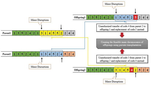
A new solution procedure is developed in this section based on the basic idea of the NSGA-II approach to deal with all features of the considered problem. The main steps of the proposed solution method are as follows: At first, an initial population is generated from the feasible main chromosome. A population of sub chromosomes is generated for each of the main chromosomes using a floating operator and the best sub chromosome for the main chromosome is selected based on the calculation of bi-objective functions value. Then, the dominate matrix is created and the rank of the Pareto front is determined for each chromosome with the computing of the crowding distance. Eventually, the next generation is selected through tournament selection. The population of feasible main chromosomes of offsprings is created using the crossover of main chromosomes of parents’ population and generate new main chromosome of offsprings through mutation operator using swap between two random genes. Finally, the best sub chromosome is selected for the main chromosome of each offspring and a new population is being produced. The algorithm is iterated until the termination condition is satisfied. The main sections of the proposed solution approach can be described based on the Table 2 as follows:

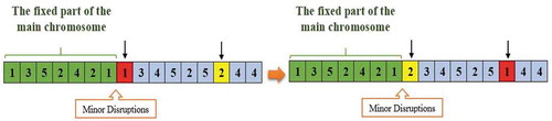
Encoding of the main chromosome structure: In order to better explanation of this structure, it is implemented on a case study presented in section 2 of this paper. Solution representation of the main chromosome structure consists of a row vector with $\sum _{w=1}^B{N}_w$ number of gens. Genes are encoded based on the corresponding number of jobs. The $w$^th job number in the main chromosome structure must be repeated $N_w$ operations and it is not allowed to repeat more or less than $N_w$. In this structure, the preserving strategy is used to make the main chromosome feasible. The structure of the main chromosome is divided into two parts such as original scheduling and reactive scheduling. The original scheduling is executed based on the initial predictive scheduling by the factory but reactive scheduling is executed based on strategies of scheduling repair. For example, in Table 2 the order of 5 jobs is received by the factory. The number of genes in the main chromosome is 16 based on the total number of operations. According to this case study, the time of occurrence of disruptions is 10 o’clock. Therefore, the stochastic start time of those operations of jobs has been done before 10 o’clock according to the initial predictive scheduling and this part is always constant in all main chromosomes. While the second part of these main chromosomes is different. In this part, a random number is selected from the set of jobs for each gene. For this purpose, if the $w$^th selected number is repeated less than or equal to $N_w$ in previous genes. Then, the $w$^th job number will be encoded in the relevant gene, otherwise, another random number is generated. The method of encoding the main chromosome structure is shown in Figure 3.

Figure 3. Encoding of the main chromosome structure

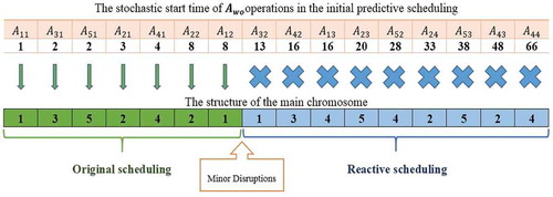
As can be seen in Figure 3, the start time of seven genes from the structure of the main chromosome that are marked in green is less than 10 o’clock. For this purpose, the numbers of jobs are transferred exactly to the corresponding gene. It is noteworthy that the blue genes are not executed according to the initial predictive scheduling. The encoding of such genes is based on a random selection of $w$^th job from the $B^{\gamma }$ set with respect to the allowable repetition limit $N_w$. For example, the first job has three operations. Thus, the number one is repeated three times in the structure of the main chromosome.

Encoding of the sub-chromosome structure: The sub chromosomes have a matrix structure. It is said that its matrix structure consists of nine rows and the number of columns is equal to the columns of the main chromosome structure. The structure of sub chromosomes is similar to main chromosomes consists of two parts such as original scheduling and reactive scheduling. The sub chromosome is encoded based on the main chromosome. Each row of this matrix represents a series of codes, which are described as follows: in row one, the number of operations is encoded based on the number of jobs in the main chromosome. It is shown that the number of stages in the second row is based on the encoding of row one related to the sub chromosome and the main chromosome. The third row depends on the encoding of the previous two rows of the sub chromosome and main chromosome, which indicates the allocation number of the machines. In the stages where there are parallel machines, the machine numbers are randomly selected and placed in the corresponding gene. The iteration number of the machine allocation number is shown in the fourth row, which is encoded based on the third row. The codes in the fifth row indicate the scheduling period of the operations of jobs. Therefore, operations of jobs receive code 1 that is in the original scheduling. The sixth row is the start time of operations if they have received code 1 in the fifth row. Therefore, their start time is based on the initial predictive scheduling. Otherwise, the start time will be generated by observing the constraints of the mathematical model. Genes take value 1 if the machine is in an idle mode between $A_{wo}$ and $A_{tp}$ in the seventh row. Sequential operations assigned to a machine are identified using the fourth row. The interval between two consecutive operations is calculated based on the sixth row and the stochastic parameter of processing time. Thereupon, the status of machines between them is defined as standby mode and idle mode. In the eighth row, genes take value 1 if the $A_{wo}$ is complete before disruption time in the original scheduling $\left(\tau \right)$. In the ninth row, genes taking value 1 if the $A_{wo}$is complete before disruption time and inaccessible to the machine in the original scheduling $\left(\tau \right)$. Thus, two rows of eight and nine are calculated based on the sixth row and the stochastic parameter of processing time. The matrix structure of the subchromosome based on the real data from a case study is shown in Figure 4.

Figure 4. Encoding of the sub chromosome structure

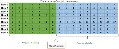
The genes shown in green are fixed for all the sub chromosomes. It is worth noting that the first three rows of the sub chromosome and main chromosome can be reached to the binary variable ${\psi }_{lwom}^{\gamma }$. From the 4^th row, the value for binary variables ${\delta }_{lwt}$ and $G_{lwoartpm}$ can be extracted along with the first three rows of subchromosome and main chromosome. Also, the binary variable ${\vartheta }_{wo}^{\tau }$ can be seen in the fifth row of the sub chromosome using the first row of the sub chromosome and main chromosome. The integer variable $\xi t_{wo}^{\gamma }$ is shown in the sixth row along with the first row of the sub chromosome and main chromosome. The binary variables ${\omega }_{wotp}$, ${\nu }_{wo}$ and ${\zeta }_{wo}$ are shown in the seventh, eighth, and ninth rows, respectively.

Steps of selection operator: In this part of the algorithm, the best chromosomes are selected through the Parto Front ranking criteria and crowding distance criteria using the value calculation of the two objective functions. The number of chromosomes selected from the initial population is calculated as (56).

(56) $N_s=round\left(POP.P_s\right)$(56)

where $P_s$ is the selection coefficient and $POP$ denoted the number of the initial population. The steps of tournament selection can be described as follows:

Step1: Calculate the value of two objective functions for all chromosomes

Step2: Determine the rank of the Pareto front through the dominate matrix. It is worth noting that, among the values of the different functions of a chromosome, at least one function has a lower value than the other chromosomes.

Step3: Calculate the crowding distance for each of the chromosomes within a Pareto front. For this purpose, we arrange the chromosomes within a Pareto front from the lowest to the highest based on the first objective function. Set the value of the first and last points of the Pareto front to infinity. The crowding distance between the middle points of the Pareto Front is calculated based on the following equation;(57) $\mathit{C}{\mathit{D}}_{\mathit{p}}=\frac{\left(\mathit{O}\mathit{F}\mathit{V}{1}_{\mathit{p}+1}-\mathit{O}\mathit{F}\mathit{V}{1}_{\mathit{p}-1}\right)+\left(\mathit{O}\mathit{F}\mathit{V}{2}_{\mathit{p}-1}-\mathit{O}\mathit{F}\mathit{V}{2}_{\mathit{p}+1}\right)}{\left(\mathit{O}\mathit{F}\mathit{V}{1}_{\mathit{l}\mathit{p}}-\mathit{O}\mathit{F}\mathit{V}{1}_{\mathit{e}\mathit{p}}\right)+\left(\mathit{O}\mathit{F}\mathit{V}{2}_{\mathit{e}\mathit{p}}-\mathit{O}\mathit{F}\mathit{V}{2}_{\mathit{l}\mathit{p}}\right)}$(57)

(57) $\mathit{C}{\mathit{D}}_{\mathit{p}}=\frac{\left(\mathit{O}\mathit{F}\mathit{V}{1}_{\mathit{p}+1}-\mathit{O}\mathit{F}\mathit{V}{1}_{\mathit{p}-1}\right)+\left(\mathit{O}\mathit{F}\mathit{V}{2}_{\mathit{p}-1}-\mathit{O}\mathit{F}\mathit{V}{2}_{\mathit{p}+1}\right)}{\left(\mathit{O}\mathit{F}\mathit{V}{1}_{\mathit{l}\mathit{p}}-\mathit{O}\mathit{F}\mathit{V}{1}_{\mathit{e}\mathit{p}}\right)+\left(\mathit{O}\mathit{F}\mathit{V}{2}_{\mathit{e}\mathit{p}}-\mathit{O}\mathit{F}\mathit{V}{2}_{\mathit{l}\mathit{p}}\right)}$(57)

In relation (57), the value of $\mathit{C}{\mathit{D}}_{\mathit{p}}$ is the crowding distance of a point $p$. In addition, $\mathit{O}\mathit{F}\mathit{V}{1}_{\mathit{l}\mathit{p}}$ is the value of the first objective function at the last point of the Pareto front and $\mathit{O}\mathit{F}\mathit{V}{1}_{\mathit{e}\mathit{p}}$ is the value of the first objective function at the first point of the Pareto front. Finally, the same definitions apply to $\mathit{O}\mathit{F}\mathit{V}{2}_{\mathit{l}\mathit{p}}$ and$\mathit{O}\mathit{F}\mathit{V}{2}_{\mathit{e}\mathit{p}}$ for the value of the second objective function.

After performing the above three steps, we randomly select two chromosomes from the initial population. Then, the chromosomes with the least rank are selected as many as need to participate in the next population. But if two chromosomes have the same rank of the Pareto front, the chromosome is passed on to the next generation with a higher crowding distance.

Steps of crossover operator: This operator is applied to the parent’s main chromosomes. Given that the original scheduling part is fixed for all the main chromosomes of parents. For this purpose, the two-point crossover method has been used to produce the main chromosomes of offsprings. The number of the parent’s main chromosomes involved in the crossover operator is calculated by equation (58)(58) $N_c=2.round\left(\frac{N_s.P_c}{2}\right)$(58) .

(58) $N_c=2.round\left(\frac{N_s.P_c}{2}\right)$(58)

where $P_c$ is the crossover coefficient. The steps of the two-point method in the crossover operator are as follows:

Step1: Random selection of two parent’s main chromosomes obtained from the selection operator

Step2: Selecting two genes to apply the two-point method of the crossover operator on the parent’s main chromosomes. It is worth noting that the first point must be set on the first gene of reactive scheduling after the occurrence of disruptions. Then, the second point is randomly selected between the first point and the last gene.

Step3: Perform the transplant operation between the two selected points in the second step on the two parent’s main chromosomes selected in the first step. It is noteworthy that the crossover operator creates infeasible main chromosomes of offsprings. For this purpose, if the $w$^th transferred number of parents is repeated less than or equal to $N_w$ in previous genes of offsprings. Then, the $w$^th job number will be encoded in the relevant gene of offsprings. Otherwise, the corresponding gene remains empty. Finally, the code for jobs that are less repetitive than the allowable limit is included in the empty gene. A schematic view of the crossover operator can be seen in Figure 5.

Figure 5. Encoding of offspring’s main chromosomes using crossover operator

Steps of mutation operator: In order to prevent premature convergence of solutions, the mutation operator uses the method of the swap between two genes to produce a new main chromosome. The operator mentioned is shown in Figure 6. The number of the offspring’s main chromosomes involved in the mutation operator is calculated by

(59) $N_m=2.round\left(\frac{N_c.P_m}{2}\right)$(59)

Figure 6. Encoding of offspring’s main chromosomes using mutation operator

where $P_m$ is the mutation coefficient. The steps of the swap method in the mutation operator are as follows:

Step1: Random selection of offspring’s main chromosomes obtained from the crossover operator

Step2: Random selection of two genes from the main chromosome of the offspring between the first gene of reactive scheduling after the occurrence of disruptions and the last gene.

Step3: Code swap between two genes from the main chromosome of the offspring.

A summary of performance of the mutation operator has been presented in Figure 6.

Steps of the floating operator: This operator is applied on sub chromosomes of the main chromosomes to enhance the power of the algorithm exploration. In this study, the floating operator has been used as an efficient method to reduce energy consumption in the framework of soft time-windows. This intelligent operator significantly reduces energy consumption using creating a float on the start time of operations. In such a way that the best status of the machine determines between the two modes of idle and standby with the best duration to stay in the above mode. Thus, this operator will reduce taxes on surplus energy consumption while maintaining the lowest level of total costs of jobs lateness penalties. The floating value is calculated based on the parameter $P_f$. The steps of the floating method in the floating operator are as follows:

Step1: Determining operations of jobs that have a free float using equation (60)(60) $F{F}_{wotp}=ma{x}_{l,m}(0,(\xi t_{tp}^{\gamma }-(\xi t_{wo}^{\gamma }+\xi p_{lwom}^{\gamma }))$(60) .

(60) $F{F}_{wotp}=ma{x}_{l,m}(0,(\xi t_{tp}^{\gamma }-(\xi t_{wo}^{\gamma }+\xi p_{lwom}^{\gamma }))$(60)

The free float $F{F}_{wotp}$ between two consecutive operations of $A_{wo}$ and $A_{tp}$ is equal to zero. Thus, there is no free float between the two operations. Otherwise, there is free float.

Step2: Creating a float between two consecutive operations based on the parameter $P_f$. Thus, the parameter $P_f$ is calculated as follows:

(61) $P_f=\mathrm{r}\mathrm{a}\mathrm{n}\mathrm{d}\left(0,\mathrm{m}\mathrm{i}\mathrm{n}\left(F{F}_{wotp}\right)\right)$(61)

Step3: Apply the floating operator on the start time of the operations of the jobs in row 6 of the sub chromosomes and row 7 being affected based on row 6. Figure 7 shows that how the floating operator performs in the proposed solution approach.

Figure 7. A schematic view of the performance of the floating operator

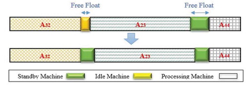
For example, creating a floating time unit at the start time of operation $A_{23}$ has changed the machine’s status from idle mode to standby mode, which consumes less energy than before.

The steps of the floating scheduling operator are shown in Figure 8. The NSGA-II using the floating scheduling operator has better quality solutions than the NSGA-II in Wu and Sun (2018) because it has a higher intelligence in a local search.

Figure 8. Flow chart of the proposed floating scheduling operator based on pNSGA-II algorithm

In the next section, a numeric example is investigated to be solved using the proposed solution approach and to analyse the performance of the floating parameter. Moreover, the performance of the proposed NSGA-II (pNSGA-II) algorithm using floating operator has been compared with the NSGA-II algorithm in Wu and Sun (2018) based on the solutions obtained from the augmented ε-constraint method.

5. Numerical analysis based on real data from a case study

All the experiments are performed on a PC with the following specifications: Intel Core (TM) 2 Duo CPU, T6570 @ 2.10 GHz, 2.00 G RAM, Win7 32 bit. For coding the proposed algorithm, Matlab software was used. These experiments were performed on real data from a case study described in Section 2 of this paper. The performance of the pNSGA-II as a Pareto-based evolutionary algorithms is strongly dependent on its parameters. We tried to tune the algorithm parameters by the Taguchi method in the design of the experiment. So, for each parameter, three different levels are defined to evaluate the influence of relevant parameters on algorithm performance. The proposed algorithm consists of 7 parameters. Each parameter was tested at three levels: low, medium, and high by the Taguchi analysis method. Test values and the final value of each parameter have been presented in Table 6.

Table 6. Parameters setting of pNSGA-II algorithm

Parameters	Test values			The best value
	Level 1	Level 2	Level 3
The population size of the main chromosomes	155	200	245	245
The population size of the sub chromosomes	12	22	34	34
$P_s$	0.40	0.50	0.60	0.60
$P_c$	0.52	0.72	0.92	0.72
$P_m$	0.30	0.40	0.50	0.50
$P_f$	1	2	3	1
Iteration	3	5	7	7

Due to the result of Table 6, the required parameters for the proposed algorithm are set as follows. The population size of the main chromosomes is considered to be 245. Also, the population size of the sub chromosomes is considered to be 34. The probabilities of selection ($P_s$), crossover ($P_c$) and mutation ($P_m$) are set as 0.60, 0.72 and 0.5, respectively. The float operator is applied to the sub chromosomes with a $\left(P_f\right)$ parameter equal to 1. The iteration has been set to 7 in order to discover the appropriate solution space and avoid long computational time. Tuning results of the parameters based on the design of experiments (DOE) is illustrated in Figure 9.

Figure 9. A demonstration of the design of experiments using Taguchi analysis

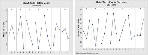
Figure 9 shows the result of the three-level plan of the Taguchi test for the seven aforementioned parameters. The population size of the main chromosomes, the population of the sub chromosomes, the selection probability, the crossover probability, the mutation probability, the float operator, and the number of generations (iterations) have been denoted by A to G, respectively. The experimental design values of each parameter have been presented in Tables A1 to A4 in the appendix.

Given that the proposed NSGA-II enhanced using a floating scheduling operator is expected to have a more accurate local search, the performance of this algorithm is compared to the NSGA-II introduced by Wu and Sun (2018). This comparison is performed in terms of three well-known indicators considering the optimum Pareto front provided by the mathematical model.

The first indicator used in this evaluation is the Error Ratio (ER). The number of solutions on the final Pareto front $P{F}_{final}$ is compared to the real Pareto front $P{F}_{real}$ as the exact solutions. The ER indicator is calculated by

(62) $ER=\frac{{\sum }_{f=1}^{F}erro{r}_f}{F}$(62)

where $F$ indicates the total number of solutions on the $P{F}_{final}$. Furthermore, error solutions are expressed on the $P{F}_{final}$ with $erro{r}_f$. If the $f^{th}$ solution of the $P{F}_{final}$ coincides with solution of the $P{F}_{real}$, $erro{r}_f$ takes value 0. Otherwise, it takes value 1. The lower values of $ER$ demonstrates that the $P{F}_{final}$ obtained by the meta-heuristic algorithm has less error than the $P{F}_{real}$ provided by the exact method.

The second indicator used in this evaluation is the Generational Distance (GD). The distance of each solution from the $P{F}_{final}$ is calculated from all $R{E}^{th}$ solutions of the $P{F}_{real}$ and the sum of the shortest distances is obtained by

(63) $GD=\frac{\sqrt{{\sum }_f^{F}min\left({\left(OFV{1}_f-OFV{1}_{RE}\right)}^2+{\left(OFV{2}_f-OFV{2}_{RE}\right)}^2\right)}}{F}$(63)

According to this relation, the GD metric indicates a shorter distance between the $P{F}_{final}$ and the $P{F}_{real}$. In other words, decreasing the value of the GD indicator represents the increase in the quality of the solutions on the $P{F}_{final}$.

The third important indicator for evaluating the proposed algorithm is the Overall Non-Dominated Vector Generation Ratio (ONVGR) that is calculated as (64).

(64) $ONVGR\stackrel{\mathrm{\Delta }}{=}\frac{F}{RE}$(64)

where the total number of solutions on $P{F}_{final}$ and $P{F}_{real}$ are shown with $F$ and $RE$ respectively. When ONVGR = 1, it shows that the same number of solutions have been found in both $P{F}_{final}$ and $P{F}_{real}$. However, it does not infer that $F=RE$. This metric requires the optimum Pareto front as $RE$. In order to evaluate the performance of the pNSGA-II algorithm, the proposed optimisation method is compared to NSGA-II in Wu and Sun (2018), and the augmented ε-constraint method. In Figure 10, the Pareto front of the NSGA-II algorithm in Wu and Sun (2018), and the pNSGA-II algorithm is carefully evaluated based on the optimal Pareto front. Therefore, the results of this evaluation are reported in Table 7 based on three important indicators such as ER, GD, and ONVGR.

Figure 10. Evaluation of the Pareto front related to the pNSGA-II algorithm

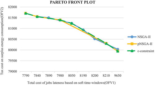
Table 7. Comparison the result of solving the small- and medium-sized cases

Cases	Specification		Method	CPU Time (Seconds)	Indicators
	Total number of jobs	Total number of operations			ER	GD	ONVGR
Case 1	5	16	ε-constraint	295	0	0	1
			NSGA-II	1171	0.66	69.09	1
			pNSGA-II	848	0	0	0.83
Case 2	7	22	ε-constraint	410	0	0	1
			NSGA-II	1472	0.68	72.38	0.90
			pNSGA-II	923	0	0	0.90
Case 3	9	29	ε-constraint	611	0	0	1
			NSGA-II	1719	0.65	75.12	0.83
			pNSGA-II	1087	0	0	0.91
Case 4	11	34	ε-constraint	972	0	0	1
			NSGA-II	2138	0.64	78.89	0.83
			pNSGA-II	1298	0.05	53.34	0.94
Case 5	13	38	ε-constraint	1644	0	0	1
			NSGA-II	2529	0.59	81.09	0.86
			pNSGA-II	1402	0.05	76.43	0.90
Case 6	15	44	ε-constraint	2946	0	0	1
			NSGA-II	3023	0.73	140.91	0.85
			pNSGA-II	1730	0.07	133.02	0.92
Case 7	17	53	ε-constraint	3806	0	0	1
			NSGA-II	3392	0.77	198.18	0.82
			pNSGA-II	2039	0.09	147.94	0.91
Case 8	19	60	ε-constraint	4536	0	0	1
			NSGA-II	4045	0.74	271.88	0.88
			pNSGA-II	2879	0.07	163.41	0.93
Case 9	23	91	ε-constraint	6314	0	0	1
			NSGA-II	5791	0.76	337.03	0.88
			pNSGA-II	3267	0.08	209.86	0.92
Case 10	26	102	ε-constraint	7526	0	0	1
			NSGA-II	6199	0.72	461.98	0.82
			pNSGA-II	3899	0.10	334.23	0.94

As can be seen in Figure 10, the Pareto front of pNSGA-II corresponds to the real Pareto front provided by the ε-constraint method. Table 7 reports the result of two algorithms in comparison to the result of the exact solution provided by the augmented ε-constraint in terms of CPU time, ER, GD, and ONVGR for 6 cases of small size and 4 cases of medium size. For all cases, the total number of machines and the total number of stages are 7 and 4, respectively. All experiments are conducted 30 runs and the best results have been reported for 10 cases.

As shown in Table 7, the pNSGA-II algorithm performs better than the NSGA-II algorithm in terms of CPU time and evaluation indicators in small- and medium-sized cases. It is important to note that determining the floating parameter is very important because increasing the value of the floating parameter does not indicate better performance in the proposed NSGA-II algorithm. Therefore, an optimal value of the parameter $P_f$ is required. In Figure 11, sensitivity analysis on the GD indicator is performed based on changes in the $P_f$ parameter.

Figure 11. Sensitivity analysis on the floating parameter in the pNSGA-II algorithm

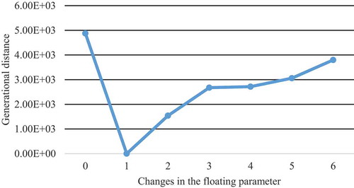
In Figure 11, the average performance of five runs for the GD indicator is considered for each floating parameter setting. As the figure shows, increasing the floating parameter from 1 to 6 makes the GD indicator worse. Therefore, the adjusted value for the floating parameter (i.e., 1) is the best value to solve the problem in this case study.

In order to better demonstrate the performance of the pNSGA-II algorithm, we solved six cases of large size. Due to the complexity of the case, it is impossible to obtain the optimum Pareto set in a reasonable time for real-world instances. Hence, some other comparison metrics should be used for result analysis that does not require to the optimum Pareto solutions. In this way, two popular indicators are illustrated and used to evaluate the efficiency of two algorithms in solving the case in real-world dimensions. The first indicator is the Overall Non-dominated Vector Generation (ONVG). The ONVG is a popular metric that presents the number of non-dominated solutions provided by an algorithm.

The second indicator used in this evaluation is Diversification (D). Diversification is another important metric in evolutionary the performance of multi-objective optimisation algorithms in which the Pareto optimal set is not known. The diversification mechanism in the algorithm is based on the extent of the solutions on the $P{F}_{final}$, which is calculated as the following :

(65) $D=\sqrt{\sum _f^{F}max\left(\left|OFV{1}_f-OFV{1}_f\right|+\left|OFV{2}_f-OFV{2}_f\right|\right)}$(65)

Moreover, $\left|OFV{1}_f-OFV{1}_f\right|+\left|OFV{2}_f-OFV{2}_f\right|$ demonstrates the distance between the two non-dominated solutions $f$ and $f$ on a $P{F}_{final}$that is calculated as Euclidean distance. Therefore, increasing diversification leading to a widespread of solutions in the parametric space. In Table 8, the evaluation output is reported based on the CPU time and value of the indicators including D and ONVG for 6 cases of large size.

Table 8. Result comparison in solving the large-sized instances

Cases	Specification		Method	CPU Time (Seconds)	Indicators
	Total number of jobs	Total number of operations			D	ONVG
Case 11	40	86	NSGA-II	10,210	4619.63	74
			pNSGA-II	7213	4931.23	93
Case 12	50	113	NSGA-II	11,909	5529.12	113
			pNSGA-II	8544	5525.98	120
Case 13	60	142	NSGA-II	13,810	5805.28	106
			pNSGA-II	9882	6581.02	146
Case 14	70	182	NSGA-II	16,121	6241.12	121
			pNSGA-II	10,981	6922.54	148
Case 15	80	199	NSGA-II	17,913	8490.19	143
			pNSGA-II	11,571	8698.81	169
Case 16	90	213	NSGA-II	19,519	9820.09	153
			pNSGA-II	12,812	9960.87	181

How to contract with the customer is always very important in a make-to-order (MTO) system. Another important challenge for managers is to reduce the contract-related costs, especially under uncertainty and disruptions. Both of the jobs lateness costs and tax costs on surplus energy consumption are dependent on the soft time-windows. Therefore, determining proper soft time-windows for the due date is important to reduce energy consumption costs in such industries and to make production profitable. In this way, a sensitivity analysis has been done on the time window changes. Table 9 and Figure 12 demonstrate the different conditions of Pareto front solutions according to changes in soft time-windows based on the Hypervolume indicator. The Hypervolume indicator is well known as an interesting indicator in tackling the bi-objective optimisation problems since it is a refinement of the Pareto dominance relation. This indicator guides to exploration of the objective space regions based on a reference point and at the same time have the property of being a refinement of the Pareto dominance relation (Auger et al. 2012).

Table 9. Sensitivity analysis on soft time-windows based on hypervolume indicator

Soft time window changes	Pareto Solutions	Reference Point	Hypervolume
−3	(10,700,81,708),(10,840,81,552),(13,060,80,304)	(5000,79,000)	18,687,760
−2	(9730,81,552),(10,200,81,084)		13,050,440
−1	(8760,83,580),(8860,81,864),(8900,81,396), (9180,80,304), (12,410,79,944)		21,017,280
0	(7790,81,708),(7840,81,552),(7980,81,396), (8210,80,304),(9650,79,944)		9,677,640
1	(6960,85,479),(7010,81,552),(7340,81,084), (9440,80,304)		16,252,560
2	(6180,85,479),(6230,81,864),(6280,81,708), (6380,81,396), (6420,80,304),(7620,79,944)		9,348,380
3	(5400,86,727),(5450,81,552),(5500,80,304)		3,283,600

Figure 12. Sensitivity analysis on the soft time-windows based on hypervolume indicator

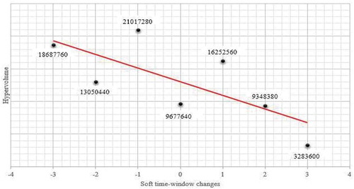
The value of the Hypervolume indicator has been reported in Table 9 according to the changes of soft time-windows from −3 to +3. In addition, Figure 12 represents the reduction rate of the Hypervolume indicator as to the upper and lower bounds of the time-window increase.

To ensure that the result of the pNSGA-II is significantly better than the NSGA-II, some statistical tests are performed on the results obtained from 30 times run for each instance. To this end, the two-sample T-test has been done on the equality hypothesis (H0: ${\mu }_0={\mu }_1$against H1:${\mu }_0<{\mu }_1$). However ${\mu }_0$ and ${\mu }_1$ are average of indicators of the pNSGA-II and NSGA-II, respectively, in 30 times solving of each instance. Table 10 shows a summary result of these tests. Observing the result, the pNSGA-II significantly outperformed the NSGA-II in terms of GD in solving the case with 10 different dimensions.

Table 10. Statistical test on equality of means GD metric for two algorithms

Cases	Descriptive statistics				Estimation for difference		Test
	pNSGA-II		NSGA-II		Difference	95%lower bound for difference	T-value	P-value
	Mean	Std. deviation	Mean	Std. deviation
Case 1	3.91	1.32	69.75	1.49	65.84	65.23	180.9	.000
Case 2	5.61	1.90	73.51	2.30	67.90	66.99	124.78	.000
Case 3	6.79	2.30	76.88	2.39	70.09	69.07	115.63	.000
Case 4	54.24	1.97	80.31	2.33	26.07	25.13	46.73	.000
Case 5	77.26	1.45	82.19	1.93	4.93	4.19	11.19	.000
Case 6	134.15	2.23	141.97	2.20	7.81	6.85	13.63	.000
Case 7	148.68	1.35	198.98	1.61	50.29	49.65	131.10	.000
Case 8	163.84	0.84	272.34	1.02	108.49	108.08	449.48	.000
Case 9	210.15	0.76	337.51	1.02	127.35	126.96	547.51	.000
Case 10	334.54	0.64	462.27	0.84	127.72	127.4	656.05	.000

Similarly, this statistical test was performed on the diversification indicator ($D$). More values of this metric indicate better performance of the relevant algorithm. Therefore, the two-sample T-test has been done on the equality hypothesis as (H0: ${\mu }_0={\mu }_1$against H1:${\mu }_0>{\mu }_1$). While, ${\mu }_0$ and ${\mu }_1$ are average of indicator $D$ calculated for the pNSGA-II and NSGA-II, respectively, in 30 times solving of each instance.

The result of this test has been addressed in Table 11. Calculating this indicator doesn’t require the optimum solutions and so, we performed this assessment for large-sized instances. Due to this result, the pNSGA-II has significantly outperformed the NSGA-II in solving five test cases of six instances.

Table 11. Statistical test on equality of means D metric for two algorithms

Cases	Descriptive statistics				Estimation for difference		Test
	pNSGA-II		NSGA-II		Difference	95%lower bound for difference	T-value	P-value
	Mean	Std. deviation	Mean	Std. deviation
Case 11	4931.11	0.40	4619.08	1	312.03	311.53	1039.14	.000
Case 12	5525.83	0.66	5526.79	3.36	0.98	−0.07	1.58	.062
Case 13	6580.83	0.63	5804.70	1.51	776.13	775.62	2592.72	.000
Case 14	6922.24	0.78	6240.70	1.23	681.53	681.09	2564.17	.000
Case 15	8698.52	0.80	8489.76	1.33	208.77	208.29	735.23	.000
Case 16	9960.52	0.84	9819.62	1.64	140.90	140.33	417.50	.000

In summary, The p-values of the statistical tests have been reported in Tables 10 and 11. As a result, the rationale of the proposed algorithm better performance is mainly because of enhancing the algorithm to a greedy heuristic local search in the algorithm which makes it more powerful to explore better much more efficiently in a proper direction which is achieved by the floating operator added in the proposed NSGA-II algorithm.

6. Conclusion

In this paper, the problem of flexible job shop scheduling was investigated under two types of uncertainties during production. We adjusted the problem for a real case study in the casting-based industry that almost uses high-powered machines to provide the optimal energy consumption. The problem was described clearly with the parameters and decision variables and then, a new bi-objective mathematical model was introduced to formulate it. Then, the non-linear model was modified to a linear MIP version. This model was developed for make-to-order (MTO) production systems with high-powered machines under uncertainty. The problem was conducted considering two conflicting objective functions of jobs lateness total costs and tax costs on surplus energy consumption. Two strategies were proposed including stochastic scheduling and reactive scheduling relevant to two different kinds of uncertainties with a known probability distribution and without any known probability distribution. A new solution approach was introduced based on the NSGA-II using a proposed floating operator. This operator causes enhancing the algorithm exploration to perform better local search throughout feasible solution space. In other words, the operator allows operations of the job to be floating within a certain range and find the best value of the objective function in local feasible spaces. It was shown that the proposed algorithm provided a set of solutions on the Pareto front close to the result of the exact method that was obtained using an augmented ε-constraint method. Moreover, the results demonstrated that the proposed solution approach outperforms the NSGA-II algorithm in Wu and Sun (2018).

To ensure the significant difference between the pNSGA-II and the NSGA-II, some statistical tests were performed on two indicators of DG and D. To this end, each of the 16 test cases was solved 30 times and equality of means was investigated using a two-sample T-test. The results demonstrated outperforming the pNSGA-II in solving 15 test cases out of a total of 16 instances.

In summary, the results of this research can lead to better management approaches in how to make a contract with the customers. However, the bargaining power with the customer in order to get more time to deliver orders can significantly reduce late penalties. On the other hand, it can also lead to a decrease in the energy consumption of machines. The solutions provided by the model indicated that how we can reduce total production costs by readjusting the soft time-windows range. It is worth noting that using a floating operator in the NSGA-II algorithm, makes the algorithm smart to do a local search heuristically in the feasible space.

As an interesting future study, it is worthwhile to develop the problem by considering release time and machine eligibility. Moreover, exploring other efficient hybrid solution algorithms may enhance the performance of the solution approach which can be recommended as a direction for further work.

Disclosure Statement

The authors do hereby declare that there is no conflict of interests of other works regarding the publication of this paper.

Additional information

Funding

The study is not funded by any agency.

Notes on contributors

Behnam Ayyoubzadeh

Behnam Ayyoubzadeh is currently a Ph.D. candidate from the Islamic Azad University, North Tehran Branch since 2018. He received his B.Sc. in Industrial Engineering from the Islamic Azad University, Karaj Branch in 2011. Also, He received his M.Sc. in Industrial Engineering from the Islamic Azad University, Karaj Branch in 2013. His main areas of research are the modelling of scheduling (especially job shop) and production planning and control. He published more than 10 papers in reputable academic journals and conferences.

Sadoullah Ebrahimnejad

Sadoullah Ebrahimnejad is an Associate Professor of Industrial Engineering at Islamic Azad University – Karaj Branch in Iran. He received his B.Sc. degree from Iran University of Science & Technology in 1986, M.Sc. degree from Amirkabir University of Technology in 1993, and Ph.D. degree from Islamic Azad University - Science & Research Branch in Tehran in 2001. His research interests are Fuzzy MADM/MODM, SCM, Operations management, Optimization models, Risk management, Multi-criteria network optimization. He published more than 90 papers in reputable academic journals and conferences.

Mahdi Bashiri

Mahdi Bashiri holds a BSc in Industrial Engineering from Iran University of Science and Technology, MSc and PhD from Tarbiat Modares University. He is a recipient of the 2013 young national top scientist award from the Academy of Sciences of the Islamic Republic of Iran. He has served as a professor of Industrial Engineering at Shahed University and an assistant professor in Business analytics at Coventry University. His research interests are sustainable supply chain network design, heuristic and matheuristic algorithms, and decision making. He has published more than 190 papers in reputable academic journals and conferences.

Vahid Baradaran

Vahid Baradaran received his Ph.D. degree from Tarbiat Modares University in the industrial engineering field in 2010. He is an associate professor at Islamic Azad University, Tehran North Branch. Since he worked in university, he taught many courses in Operation Research, Statistics, Decision Making, Multivariate Statistical Analysis, and Data Mining in Master Science, and PhD courses.

Seyed Mohammad Hassan Hosseini

Seyed Mohammad Hassan Hosseini is currently principal and assistant professor of Industrial Engineering College at Shahrood University of Technology, where he has been since 2013. He received a B.Sc. from Iran University of Science and Technology in 2000, and an M.Sc. from the Amirkabir University of Technology. He received his Ph.D. in Industrial Engineering from the Payam-e-Noor University of Tehran in 2012. From 2002 to 2008 he worked at Iran Khodro Company (IKCO) as the most famous car manufactures in Middle East as an expert of quality control and also CRM department.

His main areas of research are the modelling of scheduling (especially flow shop) and production planning and control, quality engineering and management, and decision making techniques. He has published over than 40 papers in different international journals such as Journal of applied mathematical modelling, The International Journal of Advanced Manufacturing Technology, International Journal of Industrial Engineering Computations, International Journal of Supply and Operations Management, Journal of Optimization in Industrial Engineering, Journal of Industrial and Systems Engineering, Journal of applied mathematics and computations, Environment Systems and Decisions, International Journal of Productivity and Quality Management and so on.

As of 2014, Google Scholar reports over than 200 citations to his work. He has given numerous invited talks and tutorials, and is a founder of and consultant to companies involved in car making.

Appendix

Table A1. Design summary

Taguchi array	L27(3^7)
Factors	7
Runs	27
Columns of L27 (3^13) array: 1 2 3 4 5 6 7

Table A2. Experimental design levels based on Taguchi analysis

A	B	C	D	E	F	G	GD
1	1	1	1	1	1	1	48.23
1	1	1	1	2	2	2	23.34
1	1	1	1	3	3	3	15.30
1	2	2	2	1	1	1	9.30
1	2	2	2	2	2	2	35.43
1	2	2	2	3	3	3	13.23
1	3	3	3	1	1	1	7.98
1	3	3	3	2	2	2	12.72
1	3	3	3	3	3	3	6.00
2	1	2	3	1	2	3	38.23
2	1	2	3	2	3	1	30.65
2	1	2	3	3	1	2	5.80
2	2	3	1	1	2	3	55.98
2	2	3	1	2	3	1	23.98
2	2	3	1	3	1	2	10.99
2	3	1	2	1	2	3	5.34
2	3	1	2	2	3	1	18.78
2	3	1	2	3	1	2	21.82
3	1	3	2	1	3	2	6.87
3	1	3	2	2	1	3	2.23
3	1	3	2	3	2	1	5.45
3	2	1	3	1	3	2	61.32
3	2	1	3	2	1	3	12.98
3	2	1	3	3	2	1	23.87
3	3	2	1	1	3	2	18.55
3	3	2	1	2	1	3	8.45
3	3	2	1	3	2	1	15.97

Table A3. Response table for signal to noise ratios (smaller is bettter)

Level	A	B	C	D	E	F	G
1	−23.69	−22.20	−26.34	−26.23	−25.57	−20.19	−24.47
2	−25.20	−26.86	−24.16	−19.78	−23.45	−25.33	−24.57
3	−21.33	−21.16	−19.72	−24.21	−21.21	−24.71	−21.18
Delta	3.87	5.70	6.62	6.45	4.34	5.14	3.39
Rank	6	3	1	2	5	4	7

Table A4. Response table for means

Level	A	B	C	D	F	F	G
1	19.06	19.57	25.66	24.53	27.98	14.20	20.47
2	23.51	27.45	19.51	13.16	18.73	24.04	21.87
3	17.30	12.85	14.69	22.17	13.16	21.63	17.53
Delta	6.21	14.61	10.98	11.37	14.82	9.84	4.34
Rank	6	2	4	3	1	5	7

References

- Adibi, M. A., M. Zandieh, and M. Amiri. 2010. “Multi-objective scheduling of dynamic job shop using variable neighborhood search.” Expert Systems with Applications 37 (1): 282–287. doi:10.1016/j.eswa.2009.05.001.
- Auger, A., J. Bader, D. Brockhoff, and E. Zitzler. 2012. “Hypervolume-based multiobjective optimization: Theoretical foundations and practical implications.” Theoretical Computer Science 425 (March 2012): 75–103. doi:10.1016/j.tcs.2011.03.012.
- Bagheri, M., and M. Bashiri. 2014. “A new mathematical model towards the integration of cell formation with operator assignment and inter-cell layout problems in a dynamic environment.” Applied Mathematical Modelling 38 (4): 1237–1254. doi:10.1016/j.apm.2013.08.026.
- Bruzzone, A. A. G., D. Anghinolfi, M. Paolucci, and F. Tonelli. 2012. “Energy-aware scheduling for improving manufacturing process sustainability: A mathematical model for flexible flow shops.” CIRP Annals - Manufacturing Technology 61 (1): 459–462. doi:10.1016/j.cirp.2012.03.084.
- Cai, S., X. Long, L. Li, H. Liang, Q. Wang, and X. Ding. 2019. “Determinants of intention and behavior of low carbon commuting through bicycle-sharing in China.” Journal of Cleaner Production 212 (March 2019): 602–609. doi:10.1016/j.jclepro.2018.12.072.
- Che, A., K. Lv, E. Levner, and V. Kats 2015. “Energy consumption minimization for single machine scheduling with bounded maximum tardiness.” ICNSC 2015–2015 IEEE 12th International Conference on Networking, Sensing and Control Taiwan, 146–150. doi:10.1109/ICNSC.2015.7116025.
- Che, A., X. Wu, J. Peng, and P. Yan. 2017. “Energy-efficient bi-objective single-machine scheduling with power-down mechanism.” Computers and Operations Research 85 (September 2017): 172–183. doi:10.1016/j.cor.2017.04.004.
- Chen, J., L. Wang, and Z. Peng. 2019. “A collaborative optimization algorithm for energy- efficient multi-objective distributed no-idle fl ow-shop scheduling.” Swarm and Evolutionary Computation 50 (November2019): 100557. doi:10.1016/j.swevo.2019.100557.
- Cheng, J., F. Chu, M. Liu, P. Wu, and W. Xia. 2017. “Bi-criteria single-machine batch scheduling with machine on/off switching under time-of-use tariffs.” Computers and Industrial Engineering 112 (October 2017): 721–734. doi:10.1016/j.cie.2017.04.026.
- Cheng, J., F. Chu, and M. Zhou. 2018. “An Improved Model for Parallel Machine Scheduling Under Time-of-Use Electricity Price.” IEEE Transactions on Automation Science and Engineering 15 (2): 896–899. doi:10.1109/TASE.2016.2631491.
- Chryssolouris, G., and V. Subramaniam. 2001. “Dynamic scheduling of manufacturing job shops using genetic algorithms.” Journal of Intelligent Manufacturing 12 (3): 281–293. doi:10.1023/A:1011253011638.
- Dai, M. 2015. “Research on Energy-efficient Process Planning and Scheduling.” Doctor of Philosophy. Nanjing University of Aeronautics and Astronautics.
- Dai, M., D. Tang, A. Giret, and M. A. Salido. 2019. “Multi-objective optimization for energy-efficient flexible job shop scheduling problem with transportation constraints.” Robotics and Computer Integrated Manufacturing 59 (October 2019): 143–157. doi:10.1016/j.rcim.2019.04.006.
- Dai, M., D. Tang, A. Giret, M. A. Salido, and W. D. Li. 2013. “Energy-efficient scheduling for a flexible flow shop using an improved genetic-simulated annealing algorithm.” Robotics and Computer-Integrated Manufacturing 29 (5): 418–429. doi:10.1016/j.rcim.2013.04.001.
- Danielle, M. Tendall and Claudia R. Binder. 2011. “Nuclear Energy in Europe: Uranium Flow Modeling and Fuel Cycle Scenario Trade-Offs from a Sustainability Perspective.” Environmental Science & Technology 45 (6): 2442–2449. doi:10.1021/es103270a.
- Deb, K., A. Pratap, S. Agarwal, and T. Meyarivan. 2002. “A fast and elitist multiobjective genetic algorithm: NSGA-II.” IEEE Transactions on Evolutionary Computation 6 (2): 182–197. doi:10.1109/4235.996017.
- Duflou, J. R., J. W. Sutherland, D. Dornfeld, C. Herrmann, J. Jeswiet, S. Kara, M. Hauschild, and K. Kellens. 2012. “Towards energy and resource efficient manufacturing: A processes and systems approach.” CIRP Annals - Manufacturing Technology 61 (2): 587–609. doi:10.1016/j.cirp.2012.05.002.
- Fu, Y., G. Tian, A. M. Fathollahi-fard, A. Ahmadi, and C. Zhang. 2019. “Stochastic multi-objective modelling and optimization of an energy-conscious distributed permutation flow shop scheduling problem with the total tardiness constraint.” Journal of Cleaner Production 226 (July 2019): 515–525. doi:10.1016/j.jclepro.2019.04.046.
- Gao, J., M. Gen, and L. Sun. 2006. “Scheduling jobs and maintenances in flexible job shop with a hybrid genetic algorithm.” Journal of Intelligent Manufacturing 17 (4): 493–507. doi:10.1007/s10845-005-0021-x.
- Gao, J., M. Gen, L. Sun, and X. Zhao. 2007. “A hybrid of genetic algorithm and bottleneck shifting for multiobjective flexible job shop scheduling problems.” Computers and Industrial Engineering 53 (1): 149–162. doi:10.1016/j.cie.2007.04.010.
- Gao, J., L. Sun, and M. Gen. 2008. “A hybrid genetic and variable neighborhood descent algorithm for flexible job shop scheduling problems.” Computers and Operations Research 35 (9): 2892–2907. doi:10.1016/j.cor.2007.01.001.
- Gen, M., J. Gao, and L. Lin. 2009. “Multistage-based genetic algorithm for flexible job-shop scheduling problem.” Studies in Computational Intelligence 187: 183–196. doi:10.1007/978-3-540-95978-6_13.
- Hafezalkotob, A. 2017. “Competition, cooperation, and coopetition of green supply chains under regulations on energy saving levels.” Transportation Research Part E: Logistics and Transportation Review 97 (January 2017): 228–250. doi:10.1016/j.tre.2016.11.004.
- He, Y., Y. Li, T. Wu, and J. W. Sutherland. 2015. “An energy-responsive optimization method for machine tool selection and operation sequence in fl exible machining job shops.” Journal of Cleaner Production 87 (January 2015): 245–254. doi:10.1016/j.jclepro.2014.10.006.
- Herroelen, W., and R. Leus. 2004. “Robust and reactive project scheduling: A review and classification of procedures.” International Journal of Production Research 42 (8): 1599–1620. doi:10.1080/00207540310001638055.
- Herroelen, W., and R. Leus. 2005. “Project scheduling under uncertainty: Survey and research potentials.” European Journal of Operational Research 165 (2): 289–306. doi:10.1016/j.ejor.2004.04.002.
- Ho, N. B., and J. C. Tay 2004. “GENACE: An efficient cultural algorithm for solving the flexible job-shop problem.” Proceedings of the 2004 Congress on Evolutionary Computation, CEC2004, USA, 2( July 2004), 1759–1766. doi:10.1109/cec.2004.1331108.
- Jia, Z., Y. Wang, C. Wu, Y. Yang, and X. Zhang. 2019. “Multi-objective energy aware batch scheduling using ant colony optimization algorithm.” Computers & Industrial Engineering 131 (May 2019): 41–56. doi:10.1016/j.cie.2019.03.033.
- Kall, P., and S. W. Wallace. 1994. John Wiley and Sons Ltd: Stochastic programming.
- Kianfar, K., S. M. T. Fatemi Ghomi, and A. Oroojlooy Jadid. 2012. “Study of stochastic sequence-dependent flexible flow shop via developing a dispatching rule and a hybrid GA.” Engineering Applications of Artificial Intelligence 25 (3): 494–506. doi:10.1016/j.engappai.2011.12.004.
- Lei, D. 2010. “A genetic algorithm for flexible job shop scheduling with fuzzy processing time.” International Journal of Production Research 48 (10): 2995–3013. doi:10.1080/00207540902814348.
- Lei, D., L. Gao, and Y. Zheng. 2017. “A Novel Teaching-Learning-Based Optimization Algorithm for Energy-Efficient Scheduling in hybrid flow shop.” IEEE Transactions on Engineering Management 65 (2): 330–340. doi:10.1109/TEM.2017.2774281.
- Li, K., and B. Lin. 2016. “Impact of energy conservation policies on the green productivity in China’s manufacturing sector: Evidence from a three-stage DEA model.” Applied Energy 168 (April 2016): 351–363. doi:10.1016/j.apenergy.2016.01.104.
- Li, M., D. Lei, and J. Cai. 2019. “Two-level imperialist competitive algorithm for energy-ef fi cient hybrid fl ow shop scheduling problem with relative importance of objectives.” Swarm and Evolutionary Computation 49 (September 2019): 34–43. doi:10.1016/j.swevo.2019.05.006.
- Liu, A.-J., Y. Yang, Q.-S. Xing, H. Lu, Y.-D. Zhang, Z.-Y. Zhou, G.-H. Wu, and X.-H. Zhao. 2011. “Dynamic scheduling on multi-objective flexible job shop.” Computer Integrated Manufacturing Systems 17: 2629–2637.
- Liu, Z., S. Guo, and L. Wang. 2019. “Integrated green scheduling optimization of flexible job shop and crane transportation considering comprehensive energy consumption.” Journal of Cleaner Production 211 (February 2019): 765–786. doi:10.1016/j.jclepro.2018.11.231.
- Long, X., C. Wu, J. Zhang, and J. Zhang. 2018. “Environmental efficiency for 192 thermal power plants in the Yangtze River Delta considering heterogeneity: A metafrontier directional slacks-based measure approach.” Renewable and Sustainable Energy Reviews 82 (February 2018): 3962–3971. doi:10.1016/j.rser.2017.10.077.
- Luo, S., L. Zhang, and Y. Fan. 2019. “Energy-efficient scheduling for multi-objective flexible job shops with variable processing speeds by grey wolf optimization.” Journal of Cleaner Production 234 (October 2019): 1365–1384. doi:10.1016/j.jclepro.2019.06.151.
- Mansouri, S. A., E. Aktas, and U. Besikci. 2016. “Green scheduling of a two-machine flowshop: Trade-off between makespan and energy consumption.” European Journal of Operational Research 248 (3): 772–788. doi:10.1016/j.ejor.2015.08.064.
- Mouzon, G., and M. B. Yildirim. 2008. “A framework to minimise total energy consumption and total tardiness on a single machine.” International Journal of Sustainable Engineering 1 (2): 105–116. doi:10.1080/19397030802257236.
- Mouzon, G., M. B. Yildirim, and J. Twomey. 2007. “Operational methods for minimization of energy consumption of manufacturing equipment.” International Journal of Production Research 45 (18–19): 4247–4271. doi:10.1080/00207540701450013.
- Pach, C., T. Berger, Y. Sallez, T. Bonte, E. Adam, and D. Trentesaux. 2014. “Reactive and energy-aware scheduling of flexible manufacturing systems using potential fields.” Computers in Industry 65 (3): 434–448. doi:10.1016/j.compind.2013.11.008.
- Rey, G. Z., A. Bekrar, D. Trentesaux and B,-H. Zhou. 2015. “Solving the flexible job-shop just-in-time scheduling problem with quadratic earliness and tardiness costs.” The International Journal of Advanced Manufacturing Technology 81: 1871–1891. doi:10.1007/s00170-015-7347-0.
- Shrouf, F., J. Ordieres-Meré, A. García-Sánchez, and M. Ortega-Mier. 2014. “Optimizing the production scheduling of a single machine to minimize total energy consumption costs.” Journal of Cleaner Production 67 (March 2014): 197–207. doi:10.1016/j.jclepro.2013.12.024.
- Suwa, H., and H. Sandoh. 2007. “Capability of cumulative delay based reactive scheduling for job shops with machine breakdowns.” Computers and Industrial Engineering 53 (1): 63–78. doi:10.1016/j.cie.2007.04.002.
- Tang, Z., M. Warkentin, and L. Wu. 2019. “Understanding employees’ energy saving behavior from the perspective of stimulus-organism-responses.” Resources, Conservation and Recycling 140 (January 2019): 216–223. doi:10.1016/j.resconrec.2018.09.030.
- van Zon, A., and I. H. Yetkiner. 2003. “An endogenous growth model with embodied energy-saving technical change.” Resource and Energy Economics 25 (1): 81–103. doi:10.1016/S0928-7655(02)00018-0.
- Wu, X. 2008. “Research on flexible job shop dynamic scheduling problem.” Journal of System Simulation 20 (14): 3828–3832.
- Wu, X., and Y. Sun. 2018. “A Green Scheduling Algorithm for Flexible Job Shop with Energy-Saving Measures.” Journal of Cleaner Production 172 (January 2018): 3237–3248. doi:10.1016/j.jclepro.2017.10.342.
- Wu, X., and S. Wu. 2017. “An elitist quantum-inspired evolutionary algorithm for the flexible job-shop scheduling problem.” Journal of Intelligent Manufacturing 28 (6): 1441–1457. doi:10.1007/s10845-015-1060-6.
- Wu, X., and A. Che. 2020. “Energy-efficient no-wait permutation flow shop scheduling by adaptive multi-objective variable neighborhood search.” Omega 94 (July 2020): 102117. doi:10.1016/j.omega.2019.102117.
- Yang, T., L. Zhao, W. Li, and A. Y. Zomaya. 2020. “Reinforcement learning in sustainable energy and electric systems : A survey.” Annual Reviews in Control 49: 145–163. doi:10.1016/j.arcontrol.2020.03.001.
- Zhang, H., L. Li, P. Zhou, J. Hou, and Y. Qiu. 2014. “Subsidy modes, waste cooking oil and biofuel: Policy effectiveness and sustainable supply chains in China.” Energy Policy 65 (February 2014): 270–274. doi:10.1016/j.enpol.2013.10.009.
- Zhang, R., and R. Chiong. 2016. “Solving the energy-efficient job shop scheduling problem: A multi-objective genetic algorithm with enhanced local search for minimizing the total weighted tardiness and total energy consumption.” Journal of Cleaner Production 112 (January 2016): 3361–3375. doi:10.1016/j.jclepro.2015.09.097.