Electricity demand and price forecasting model for sustainable smart grid using comprehensive long short term memory

ABSTRACT

This paper proposes an electricity demand and price forecast model of the smart city large datasets using a single comprehensive Long Short-Term Memory (LSTM) based on a sequence-to-sequence network. Real electricity market data from the Australian Energy Market Operator (AEMO) is used to validate the effectiveness of the proposed model. Several simulations with different configurations are executed on actual data to produce reliable results. The validation results indicate that the devised model is a better option to forecast the electricity demand and price with an acceptably smaller error. A comparison of the proposed model is also provided with a few existing models, Support Vector Machine (SVM), Regression Tree (RT), and Neural Nonlinear Autoregressive network with Exogenous variables (NARX). Compared to SVM, RT, and NARX, the performance indices, Root Mean Square Error (RMSE) of the proposed forecasting model has been improved by 11.25%, 20%, and 33.5% respectively considering demand, and by 12.8%, 14.5%, and 47% respectively considering the price; similarly, the Mean Absolute Error (MAE) has been improved by 14%, 22.5%, and 32.5% respectively considering demand, and by 8.4%, 21% and 61% respectively considering price. Additionally, the proposed model can produce reliable forecast results without large historical datasets.

KEYWORDS:

• Forecasting electricity demand and price
• Lstm
• sequence-to-sequence network
• time-series data
• smart grid
• smart city

1. Introduction

During the recent decade, a large number of people are tending to live in urban areas than in rural areas. The growing population of the cities wants to avail themselves of all the cutting-edge facilities that a Smart City can provide. Smart City can regulate the challenges smartly linked with increased population to control their basic integral of life, such as energy, transport, health, and homes. Modernisation of the grid and digitisation is essential to manage, monitor, and respond to the energy problems of smart cities. Sustainable development of Smart Grid (SG) is essential for reliable and affordable electricity for smart city’s consumers. The use of information and communications technology in the electrical power supply network is the motivation for the SG and expansion for several grids to feed the demand. An SG can make effective use of the Internet of Things (IoT) to improve two-way communications between utility companies and their consumers to provide sustainable services, such as access to near real-time data to make environmentally safe and profitable decisions. Consumer demand response and energy demand balancing can be well managed by implementing sustainable demand-side management (DSM) algorithms (Yu and Hong 2016).

An SG establishes an interactive environment between electricity consumers and utility. The DSM program enables its users to manipulate their demand by instant price differences. By participating in SG operations, it provides energy consumers with demand shifting and energy saving to reduce the cost of electricity usage. However, the growing rate of different electricity sources, such as renewable energy and flexible loads (e.g. electric vehicles), and randomly changes to demand in the distribution grids, making electricity demand and pricing more complex and uncertain every day. Therefore, an accurate forecast of both electricity demand and price holds great importance in DSM and sustainable market operations management to minimise this uncertainty. Furthermore, increasing the reliability of the DSM and demand forecasting is important in electricity grid planning and demand scheduling (Khuntia, Rueda, and Van der Meijden 2018).

In general, electricity demand and price display distinctive features and clear correlations (Gao et al. 2019). Nonetheless, the electricity demand and pricing data show a few different patterns (AER Report 2018). There are different factors, such as fuel price, distribution of cheap production of the windmill and photovoltaic, social, economic, weather pattern, for such unpredicted price pattern changes (Mujeeb et al. 2018). It is noticeable that just a direct change in demand does not affect the electricity price. All these aspects make electricity forecasting a challenging problem. Therefore, electricity demand and price forecasting are important for those involved in the electricity market.

Since electricity production is not preservable like other usual products (Kuo and Huang 2018), a reliable structure is necessary to maintain sustainability among supply and demand. Due to a lack of production and wastage of electricity, there is usually a discrepancy between electricity demand and production level. During the pick time, DSM and electricity balancing is accomplished by limiting electrical device usages which ultimately affects users’ satisfaction (Jabir et al. 2018). As a result, electricity demand and price forecasting are crucial to avoid disparity between demand, supply, and related prices. It is therefore essential to improve the forecasting accuracy in terms of the possible error reduction. Table 1 is an example of the percentage differences between actual and forecasts energy consumption, by five regions in Australia, adopted from the Australian Energy Market Operator (AEMO report2019). AEMO is responsible for operating Australia’s largest gas and electricity markets and power systems, assessed annual consumption forecast accuracy (performance) by measuring the percentage difference (error) between actual and forecast values of the published energy forecast. (-ve error implies the actual is lower than forecast by %) (AEMO report 2019).

Table 1. Energy forecast accuracy (percentage error) by region from different locations in Australia (AEMO report 2019)

1-year ahead annual operational consumption accuracy (%)	Forecast in
	2014–2015	2015–2016	2016–2017	2017–2018	2018–2019
New South Wales	3.2%	1.2%	0.8%	0.1%	1.8%
South Australia	−0.2%	1.6%	−1.6%	0.8%	0.8%
Tasmania	2.3%	−3.5%	−2.4%	0.1%	−1.3%
Queensland	6.7%	−2.6%	−1.6%	−2.8%	3.1%
Victoria	0.3%	−0.5%	−5.0%	−2.5%	−3.7%

Traditional forecasting methods, such as moving average (MA) and trend analysis, becomes very difficult and limited when applied to complex non-linear systems with large time-series data set (Adhikari and Agrawal 2013). These methods are challenging for accurately measured and represented with detail dynamic operations (Adhikari and Agrawal 2013). Therefore, traditional forecasts need to be replaced by accurate and advance predictive models that can process nonlinear data and produce effective results. Deep learning algorithms provide a strong way to extract key attributes from complex variable historical electricity data to predict the demand/price efficiently. As a result, applying deep learning algorithms to process time series electricity data yields better results. Researchers have been applying deep-learning methods, such as Artificial Neural Network (ANN), that can produce excellent results in critical issues, reduce errors and improve the models’ prediction accuracy.

Therefore, the main goals of our research include the design of a single comprehensive accurate electricity demand and price forecasting method with a reduced error rate. This research proposes a sequence-to-sequence model that is commonly used for language translation (Sutskever, Vinyals, and Le 2014) and can learn variable temporal structure in the input sequence, which has been adapted for the forecasting model.

The contributions of our research work are as follows:

• Empirical analyses of electricity demand and price data are performed.

• Predictive analytics (uses LSTM-based sequence-to-sequence network) on electricity demand and price data are performed.

The arrangement of this paper is as follows: the literature review is given in Section 2. The theoretical background of this work is discussed in Section 3. Section 4 describes the LSTM network model design. Details of the dataset used for this study are described in Section 5. The modelling results and discussions are presented in Section 6. Section 7 concludes the article.

2. Literature review

Forecasting methods can be classified into two main categories, traditional statistic methods and computational intelligence methods. Traditional statistic methods use the collected time-series data of the electrical demand and price to identify the electricity usage trend. An autoregressive moving average (ARMA) model was proposed for modelling the electricity demand (Xu et al. 2018). The autoregressive integrated moving average model (ARIMA) is more accurate at short-horizon electricity demand forecasting (Ghasemi et al. 2016). In (Papalexopoulos and Hesterberg 1990), a linear regression-based statistical model approach is provided, depends on historical data for short-term system demand forecasting. The multiple linear regression model (Hong et al. 2010), which is a simple time-series technique for modelling and forecasting the set of demand or production data as a linear curve.

In (Nagbe, Cugliari, and Jacques 2018), a functional state-space model to forecast electricity demand is assigned by the system state and quantifying equations to implement it at some stage of grouping between the local and national grid. One of the drawbacks of the traditional statistical methods is that it needs suitable samples and many difficult factors to obtain the parameters required for the forecasting models (Li and Zhang 2018).

The second approach for electricity demand and price forecasting consists of computational intelligence methods, such as support vector machine (SVM) (Chen, Chang, and Lin 2004), decision tree (Tso and Yau 2007), and artificial neural network (ANN) (Roldán-Blay et al. 2013; Wang, Qi, and Liu 2019) and fuzzy logic (FL) (Khodaei et al. 2018). These methods have been very successful in recent times due to their strong non-linearity learning and modelling capabilities, which are explicit in most traditional statistical methods (Xu et al. 2018). The ANN model is currently one of the most popular methods for time-series prediction (Wang, Qi, and Liu 2019; Szkuta, Sanabria, and Dillon 1999; Park et al. 1991). In (Szkuta, Sanabria, and Dillon 1999), first used ANN with a single hidden layer to forecast the output price in Victorian (Australia) electricity market for past prices, demand, and capacity data, and also specific information related to the calendar (day code, season, holiday code, etc.).

Unlike statistical methods, ANN requires no intrinsic assumption about the data used for prediction modelling and it is also adaptive to missing data (Park et al. 1991). Moreover, to improve the training mechanism and forecasting capacity, Gao et al. (2019) proposed a forecast engine consisting of the multi-block neural network (NN) and optimised with an objective function. Besides, Ghadimi et al. (2018) have developed an improved meta-heuristic algorithm for electricity demand forecasting that depends on a novel intelligent algorithm in conjunction with a new feature selection system. Dynamic choice ANN is suggested by Wang et al. (2016) which is a hybrid of supervised and unsupervised learning for day-ahead price forecasting, to delete bad samples and look for optimal inputs. However, the ANN method needs a large number of historical data for forecasting and only efficient during training but not during validation and testing phases (Lau, Sun, and Yang 2019). Furthermore, the ANN’s performance varies greatly such as input-output correlation, as well as the correct and efficient tuning of weight and bias in the hidden and output layers (Gao et al. 2019). Moreover, ANNs also have a slow rate of self-learning convergence, making it easier to collapse into a local minimum (Wang et al. 2016).

The fuzzy logic controller (FLC) has been used in many areas and complex control systems to improve forecasting.

It is capable of making an optimal decision based on a set of inputs (Khodaei et al. 2018). In (Khodaei et al. 2018) proposed a multi-objective model for cost emission operation of an industrial consumer with help of fuzzy-based heat and power hub models. The fuzzy logic is a non-linear system that uses IF-THEN logic to work and its’ ability to give answers among ‘true’ and ‘false’ is more commonly used in temperature and machine control (Alam and Ali 2020). Therefore, computers cannot explicitly process and analyse the fuzzy system and usually requires the use of specific rules for simulation (Suganthi, Iniyan, and Samuel 2015). Moreover, it also becomes a slow system since it works by the fuzzy system which relies for each input on the numbers of inputs and the membership function (Alam and Ali 2020).

Besides ANN and SVM have been widely used to predict short-term electricity demand and price (Mohandes 2002; Jiang, Liu, and Song 2017; Wang et al. 2019; Zahid et al. 2019; Gao et al. 2019). In (Jiang, Liu, and Song 2017; Wang et al. 2019; Gao et al. 2019), SVM is used for feature selection. Feature selection is important in forecasting models, but it’s a difficult task because the size and form of input variables should be properly designed (Zahid et al. 2019). Besides, the major drawback of SVM is significant computing difficulty and parameter settings (Gao et al. 2019). As a result, it is incompatible with large-scale training data (Wang et al. 2019). In much of the current literature (Wang et al. 2019; Zahid et al. 2019), test datasets are only available for one week, which ignores the issue of special days (such as holidays) during the year, and is not indicative to produce a definite conclusion.

Furthermore, stochastic optimisation methods have been developed and have become common in forecasting. They are mostly used when the system is volatile. In a deregulated electricity market, the authors (Abedinia et al. 2019) suggested a hybrid stochastic-robust optimisation-based approach to get optimal offering, bidding strategies, and demand uncertainties of large consumers. Modelling the unknown parameters in cooling demand has been performed in (Saeedi et al. 2019) using a robust stochastic optimisations method. Based on an intelligent algorithm, Ghadimi et al. (2018) evaluated an improved metaheuristic algorithm together with a new feature selection system for electricity demand forecasting. Nevertheless, sometimes these optimisation algorithms are affected by computational complexity, a lower convergence rate, and local minimum trapping.

The author demonstrated in previous work (Yue, Dan, and Liqun 2012) that a dynamic NN is used to forecast daily electricity demand to maintain the connection between production and demand. In another literature (Pan et al. 2019), the author presented a developed backpropagation NN (BPNN) for Short-term electricity demand forecasting based on complexity decomposition technology and modified flower pollination optimisation. Calculation and training time can be accelerated by using the Extreme Learning Machine (ELM), which is very common these days to model shallow patterns (Zhang et al. 2013; Ertugrul 2016; Jiang, Liu, and Song 2017; Wang et al. 2019). ELM is a specific type of one-hidden-layer NN with no iterative process to make it faster (Ertugrul 2016).

Dehalwar et al. (2016) studied electricity demand influence factors and used weather forecasts to produce an electricity demand prediction model based on the ANN for a large urban area in Australia. Big data analytics and forecasting of electricity price data are performed in (Mujeeb et al. 2019), based on a hybrid model. Big data studied for better electricity price forecasting, in which random forest (RF) and relief-F based on grey correlation analysis (GCA) for feature redundancy, and kernel function (KF) and principal component analysis (PCA) for feature reduction, and SVM for performance classifier have been used (Wang et al. 2017). In (Andalib and Atry 2009), applied a nonlinear autoregressive exogenous (NARX) NN Model for electricity price forecasting. These study results show the improved quality of the NARX model.

Considering the aforementioned literature, many current studies have been dedicated to effectively forecasting various types of time-series. However, classical statistical approaches, such as hybrid framework (Jiang, Liu, and Song 2017), fuzzy logic (Khodaei et al. 2018), and ARIMA (Ghasemi et al. 2016), are still difficult to be used to model and forecast such non-stationary time-series.

Besides, deep NN has been integrated with time-series forecasting as a result of the ongoing enhancement of computer hardware and software, and smart city’s big data technology. Therefore, deep learning has received a growing interest among researchers for forecasting methods (LeCun, Bengio, and Hinton 2015) and effectively implemented in different time-series problems, such as language modelling (Mikolov et al. 2014), speech recognition (Graves, Mohamed, and Hinton 2013), stock market prediction (Nelson, Pereira, and de Oliveira 2017), and flood forecasting (Le et al. 2019). In (Ugurlu, Oksuz, and Tas 2018), the researchers used a recurrent neural network (RNN), which is a special kind of ANN, assessed as an important method for time-series forecasting. However, RNN showed insufficiency while training time-series with long time lags and depends on the fixed time lags to learn the computation of time-series sequence (Lipton, Berkowitz, and Elkan 2015). It is more inclined to gradient explosion and disappearance. LSTMs, are a special type of RNN, can learn long-term dependencies by remembering and capturing information of time-series for a longer time (Hochreiter and Schmidhuber 1997a).

Besides, few other methods were also integrated with ANN models to improve electricity demand or price forecasting performance, such as feature selection and genetic algorithm to optimise an LSTM model (Bouktif et al. 2018), support vector regression (SVR), stacked auto-encoders (SAEs) with the ELM (Li et al. 2017), and stacked de-noising auto-encoders with SVR (Tong et al. 2018). It is observable that the ANN-RNN based models were very common for related fields of electricity.

However, the above methods described in the literature can produce good results, their algorithms are complex and difficult. Even though the above studies all relate to demand/price forecasting in a separate category. The suggested work in this paper is different since it depends on LSTM-based sequence-to-sequence model to forecast electricity demand and price. This sequence-to-sequence model offers a stronger analysis in time-series problems by using an encoder-decoder LSTM model, which has been commonly used for language translation (Sutskever, Vinyals, and Le 2014). The encoder-decoder LSTM effectively extracts the features of the input data to make multi-step sequence predictions (Figure 2). The most comparable work to ours is the work by (Sehovac and Grolinger 2020). In energy forecasting, they used standard RNN-based sequence-to-sequence models with attention mechanisms, comparing their efficiency with various RNN cells and forecasting intervals. To produce a context vector, they first send the input sequence into the encoder RNN one-time step at a time. The decoder RNN is then used to decode this vector into a processed input sequence. Although any RNN can theoretically encode-decode the sequence, the long-term dependencies that result can lead to poor results.

To address this problem, LSTM models are more appropriate in this paper and used as sequence encoders–decoders. LSTM is particularly suitable for learning long-range dependencies, in which the conventional recurrent network fails with a large amount of sequential input data (Sutskever, Vinyals, and Le 2014). Sequence-to-sequence LSTM models enable information to be better stored in sequence data than in conventional ANNs, RNN, and SVMs (Sehovac and Grolinger 2020). Given the significant time lag seen between inputs and the respective outputs, the LSTM is capable of learning effectively regarding data of long-range temporal dependencies makes it an ideal fit for this research.

The literature reports that LSTMs support cutting-edge results in sequence-related research. Although, the model was recently used in energy and weather forecasting (Zaytar and El Amrani 2016). Its application in the area of electricity demand and price forecasting has not been used substantially. In (Marino, Amarasinghe, and Manic 2016), LSTM was compared to the sequence-to-sequence network where the latter performed better. Additionally, in (Sehovac and Grolinger 2020), sequence-to-sequence RNN showed better results than standard RNN. In a recent research (Sehovac and Grolinger 2020), a sequence-to-sequence RNN with an attention mechanism was developed for electrical load forecasting and a similar sample generation approach was designed. In (Gong et al. 2019), a short-term load forecast model based on LSTM is developed with two attention mechanisms. Their model (Sehovac and Grolinger 2020; Gong et al. 2019) is very close to the language translation model in (Sutskever, Vinyals, and Le 2014), which uses one LSTM to encode the input sequence into a fixed vector, and another LSTM to decode the target sequence from it. The attention mechanism learns to weight the frame features variable conditioned on the previous word input(s) rather than fixed weighting features from all frames (Sutskever, Vinyals, and Le 2014).

Conversely, this research uses a simpler approach using a single LSTM which learns both encoding and decoding based on the inputs given. This allows the LSTM to share weights between encoding and decoding. Therefore, this direct sequence-to-sequence model does not require any specific attention mechanism.

This study suggested different LSTM network topologies get an understanding of network architecture when dealing with big data time-series data set of smart grid to identify appropriate configurations to solve the problem. Therefore, the electricity demand and price forecast can achieve good results by using the LSTM network so that electricity producers and consumers can take proper decisions for DSM and usages respectively.

3. Theoretical background

3.1 Long Short-Term Memory (LSTM) network

The basic purpose of proposing LSTM was to avoid the problem of vanishing gradient (using gradient descent algorithm), which occurs while training of BPNN neural network (Hochreiter and Schmidhuber 1997b). All RNN follow the structure of a chain of recurring modules of NN. For regular RNNs, this recurring module (as seen in Figure 1a) will have a very simple structure, like a single tanh layer. Figure 1b shows the structure of LSTM includes three main gate structures: forget gate ($f_t$), input gate ($i_t$), and output gate ($o_t$), $x_t$ represents the input data, $h_t$represents the hidden state, $C_t$ as a cell state.

Figure 1. (a) Standard recurrent neural network (RNN) (Kuo and Huang 2018). (b). Long Short-Term Memory (LSTM) (Kuo and Huang 2018)

Figure 2. The structure of Sequence-to-Sequence Network (Sutskever, Vinyals, and Le 2014). (h,c) represents intermediate vector

An LSTM network computes a mapping from an input sequence X = ($x_1$,$x_2$, … …, $x_n$) to an output sequence Y = ($y_1$, $y_2$ … …, $y_m$). The LSTM cell computation at time t, for an input $x_t$:

(1) $f_t=\delta \left(W_f{x}_t+U_f{h}_{t-1}+b_f\right)$(1)

(2) $i_t=\delta \left(W_i{x}_t+U_i{h}_{t-1}+b_i\right)$(2)

(3) $g_t=tanh\left(W_g{x}_t+U_g{h}_{t-1}+b_g\right)$(3)

(4) $C_t=i_t\ast g_t+f_t\ast C_{t-1}$(4)

(5) $o_t=\delta \left(W_o{x}_t+U_o{h}_{t-1}+b_o\right)$(5)

(6) $h_t=o_t\ast tanh{C}_t$(6)

Where $\delta$ and tanh are the activation function, W and U are the weight of forget gate, and b is bias vector, $C_{t-1}$ and $C_t$are the cell states at time t − 1 and t.

Another reason that LSTM is a good choice for this research since it takes sequence data as input, unlike other models, such as ARMA, ELM, SVM, where lag observations need to be presented as input features (Brownlee 2018). Since LSTMs do not need fixed-size input data, they can use the time-series input to search for the perfect number of lookbacks and look for patterns on their own (Brownlee 2018).

3.2 Sequence-to-Sequence network

To forecast the values of future time steps of a sequence, a sequence-to-sequence regression LSTM network can be trained. The sequence-to-sequence architecture that is commonly used for language translation (Sutskever, Vinyals, and Le 2014), is adapted for electricity demand and price forecasting.

A typical sequence-to-sequence model takes input sequence X (encoder) of variable length and changes that in a fixed-length vector, which is then used as the input sequences for the next time step (Sutskever, Vinyals, and Le 2014). By this process, an output sequence Y (decoder) of n length is generated. In this case, at each time step of the input sequence, the LSTM network learns to forecast the value of the next n time steps. The sequence-to-sequence network architecture’s advantage is that it permits a random number of input length of previous time steps to forecast a random number of future time steps (Sutskever, Vinyals, and Le 2014). The structure of sequence-to-sequence is shown in Figure 2.

Therefore, during encoding, with input sequence X, the LSTM computes a sequence of hidden states ($h_1$,$h_2$, … …, $h_n$). During decoding it defines a distribution over the output sequence Y given the input sequence X as p(Y |X) is:

(7) $p\left(y_1,\dots ,y_m|x_1,\dots ,x_n\right)=\prod _{t=1}^{m}p(y_t|v,y_1,\dots ,y_{t-1})$(7)

Where v is fixed dimensional vector representation of the X given by the last hidden state of the LSTM, and then computing the conditional probability of Y with a standard LSTM- Language Model (LM) formulation whose initial hidden state is set to the representation vector v of input X (Sutskever, Vinyals, and Le 2014). LM is a probability distribution over sequences of input (Sutskever, Vinyals, and Le 2014). The easy model of an LM is predicting the next time step given the previous time step(s).

Figure 3 shows the step-by-step flowchart of the proposed method.

Figure 3. Flowchart of the proposed forecasting method

As shown in Figure 3, the dataset is separated into a training and testing dataset. The training dataset and testing dataset are standardised and then arranged in several input sequences. A forecasting model is established then based on the proposed model and trained dataset with defined LSTM network architecture to predict the electricity demand and price to be as precise as possible.

3.3 Measure prediction quality

Commonly used metrics to evaluate forecast accuracy are the Root Mean Squared Error (RMSE), Mean Absolute Error (MAE), and correlation coefficient value (R²) (Kuo and Huang 2018). A lower RMSE and MAE indicates a better forecasting result, which measures the difference between the actual values to the forecasting values. The R² value, which is between 0 and 1 (where 0 means no correlation and 1 means the model has no error), determines the correlation between actual and predicted values. The three error measures are defined as follows:

(8) $RMSE\left(X,h\right)=\sqrt{1\hspace{0.17em}\sum _{i=1}^m{\left(h\left(x^{\left(i\right)}\right)-y^{\left(i\right)}\right)}^2}$(8)

(9) $MAE\left(X,h\right)=1\hspace{0.17em}\sum _{i=1}^m|h(x^{\left(i\right)})-y^{\left(i\right)}|$(9)

(10) $R=\frac{{\sum }_{i=1}^m\left({\mathrm{x}}_{\mathrm{i}}-\bar{x}\right)({\mathrm{y}}_{\mathrm{i}}-\overline{\mathrm{y})}}{\sqrt{{\sum }_{i=1}^m{\left({\mathrm{x}}_{\mathrm{i}}-\bar{x}\right)}^2}\sqrt{{\sum }_{i=1}^m{\left({\mathrm{y}}_{\mathrm{i}}-\bar{\mathrm{y}}\right)}^2}}$(10)

Where considering x to be the actual values, y defining the predicted values, $\bar{x}$ defining mean of x, $\bar{y}$ defining the mean of y, X is a matrix containing all the features values, h is the prediction function and m is the total number of instances in the test set.

4. LSTM network model design

The first processing step of the LSTM network model design begins by demanding the datasets (Energy demand and price). In this study, the electricity demand and spot pricing dataset used as a separate row vector, each contains values of the accumulated electricity demand and spot price with a 30-min resolution.

A variety of random factors, such as demographic, socio-economic or cultural, weather conditions, etc., can influence the electricity demand and price behaviour. Therefore, the accuracy of original data is sometimes low and it is necessary to pre-process the original data to improve the model prediction accuracy. This study pre-processes data through standardisation. Before taking data to train the forecast model, standardise the training data to have zero mean and unit variance for a better fit, and to eliminate the training from deviating (Garreta and Moncecchi 2013). The two datasets are demanded separately for network training after standardisation.

Here, the standardised variable is $X_{stand}$ which is equal to the original variable (x), minus it’s mean ($\mu$), divided by its standard deviation ($\sigma$).

(11) $X_{stand}=\frac{X-\mu }{\sigma }$(11)

A sequential prediction is used when a sequence-to-sequence model is trained (Sutskever, Vinyals, and Le 2014). To avoid over-fitting and improve accuracy on testing data, Dropout is used as a regularisation methodology for fully connected neural network layers (Srivastava et al. 2014). Regularisation is a technique that makes small adjustments to the learning algorithm so that the model is more generalised and reduces overfitting. This effectively also increases the performance of the model on the unseen results (Wan et al. 2013). Dropout implies that a unit is temporarily dropped from the network, for all its coming and outgoing links (Medennikov and Bulusheva 2016). All elements of an output layer are stored with probability p, alternatively set to 0 with probability (1 – p). Equation 12(12) $P\left(n\right)=\left\{\begin{array}{c}1-pforn=0\\ pforn=1\end{array}\right.$(12) simply shows in this case drop unit or not (Wan et al. 2013).

(12) $P\left(n\right)=\left\{\begin{array}{c}1-pforn=0\\ pforn=1\end{array}\right.$(12)

The precision of the experiential’s result is improved by adjusting and choosing the model’s variables to produce the desired output. The architecture of the proposed forecast method is shown in Table 2. Adam (Adaptive Moment Estimation) optimiser algorithm is used for adaptive optimisation to update network weights iterative based throughout the training data (Bouktif et al. 2018). There is no exact rule for selecting the number of hidden units for an LSTM network. It generally depends on the area of application (Le et al. 2019). It can be decided by experimentation in a particular case.

Table 2. Details of the LSTM regression network model

Parameter	Details
Number of features	1
Number of responses	1
Number of hidden units	200/100/50
Initial learning rate	.005
Learn rate drop period	125
Epoch	200/250/300
Training algorithm Dropout (p)	Adam 0.5

5. Description of dataset

AEMO has an open dataset, which contains accumulated daily electricity demand (30 min MW) and price (30 min/MWh) sampling rate (AEMO 2019). The range of data for this study is 3 years, from the year 2017 January to 2019 November comprises 50,112 time-series data; and 1 year, from 2018 to 2019 November comprises 18,001 time-series data of New South Wales (NSW), Australia.

To improve the model performance, the cross-validation technique is used for the assessment of the forecasting model (Hu et al. 1999). The steps involved in cross-validation are the splitting of the dataset into two detached groups, training, and test dataset; reserving the test data; training the remaining data set, and then use the test data set for unbiased performance comparison (Hu et al. 1999). The LSTM network of this research trains on the first 90% (initial network) and tests on the last 10% of the time series sequence (Figure 4).

Figure 4. Splitting of the dataset (Wang, Qi, and Liu 2019)

The LSTM network forecasts step forward values at each time step throughout the training process. In this scenario, electricity demand and price data are the separate input as the single time-series data to the model. The LSTM network is trained individually for these two different features.

5.1 Exploratory data analysis

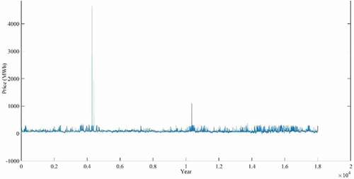
In time-series forecasting, the observed data corresponds with its previous data (Adhikari and Agrawal 2013). Therefore, each observation cannot be treated as independent data. The initial exploratory data analysis of electricity demand and pricing data can be useful for identifying trends and patterns. The accumulated electricity demand and pricing curves of 3 years (NSW) are shown in Figures 5 and 6, respectively, which follows cyclic and seasonal patterns.

Figure 5. Accumulated daily electricity demand (NSW) (Jan 2017-Nov2019)

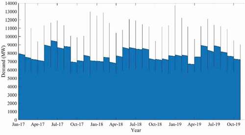
Figure 6. Accumulated daily electricity price (NSW) (Jan 2017- Nov 2019)

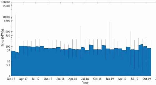
The electricity demand indicates the same months, such as January 2017, January 2018, and January 2019, display a consistent trend. This is because of the same weather (summer in Australia) during that time in different calendar years. This also reflects on the price data, which shows in Figure 6 that price was also at a peak rate due to hot summer weather.

Figure 7 displays a scatter plot of daily electricity demand and price relationship over 3 years, which are significantly affected by seasonality. Throughout the year, electricity demand shows a predictable pattern and rises at a slow steady rate unlike the electricity price that changes very randomly with a few sudden price peaks, and sparingly following any pattern. Verily weather and different seasons have a major impact on electricity demand and price.

Figure 7. Accumulated daily electricity demand and price relationship (Jan 2017- Nov 2019)

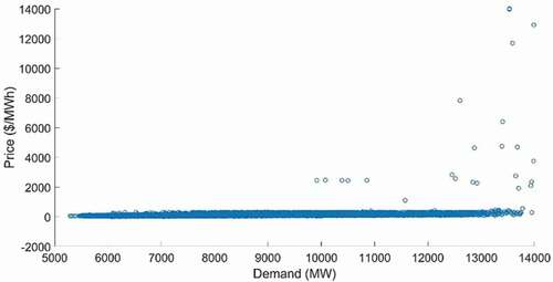
Figure 6 shows in most cases, price increases with demand increases. However, in some exceptional cases, price is much higher (sharp increase) than demand. According to the Australian Energy Regulator (AER) (AER Report 2018), for the last five years, the main factors to a short-term sharp increase in price have been rebidding and inaccurate demand forecasting. Rebidding usually occurs if there is an urgent need or sudden change in market demand, weather conditions, generator production, network restrictions, or other generators’ bids. It enables the electricity generators to update and submit new bids for more or less supply as the delivery time gets closer.

Daily electricity demand and price curves for workdays and weekends, from all the seasons of the year (2017–2019), are also represented, respectively, in Figures 8–9. As seen in these Figures 8–9, the electricity demand gap is significant between workdays and weekends. It is easily perceived that electricity demand and usages on weekends are considerably lower due to fewer activities than weekdays round the year. Figures 10–11 displays the electricity demand and price data curve for 1 year.

Figure 8. Accumulated workdays and weekend electricity demand curve 3- years (Jan 2017- Nov 2019)

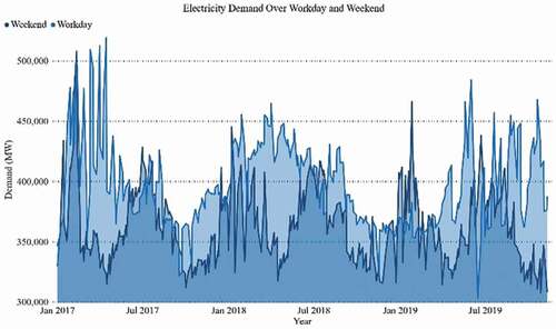
Figure 9. Accumulated workday and Weekend electricity price curve 3- years (Jan 2017- Nov 2019)

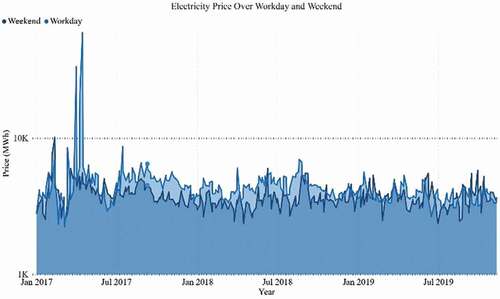
Figure 10. Accumulated daily electricity demand data for o1 year

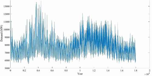
Figure 11. Accumulated daily electricity price data for 1 year

6. Forecasting model results and discussion

This section first executed several simulations of the forecasting model. Next, presents the experimental results and test results evaluation. Then, discusses the ablation study. Finally, a comparison of the proposed model is also provided with a few existing models.

Several simulations of the forecasting model are executed to establish the proposed sequence-to-sequence LSTM network model. For each dataset (electricity and price), this forecasting model has been run 9 times independently with different forecasting granularities (Table 3). These simulation results explain the performance of the proposed model in addition to the RMSE and MAE errors, a total of 36 different cases in Table 3.

Table 3. Prediction quality of the sequence-to-sequence regression LSTM network model in nine different cases and test result evaluation for electricity demand and price data

	Test Run	1	2	3	4	5	6	7	8	9
No. of Hidden unit/Epoch		200/250	100/250	50/250	200/300	100/300	50/300	200/200	100/200	50/200
1 year Electricity Demand	MAE	50.96	54.72	55.27	51.8	54.74	56.18	52.87	54.81	60.62
	RMSE	67.35	71.31	71.15	68.09	71.14	72.2	69.6	71.02	77.84
	Forecasted Highest	9522	9543	9541	9558	9488	9502	9491	9488	9558
	Observed Highest	9515	9515	9515	9515	9515	9515	9515	9515	9515
	Relative Error	0.07	0.28	0.26	0.43	0.27	0.13	0.24	0.27	0.43
3 years Electricity Demand	MAE	73.88	74.5	78.63	77.41	76.79	79.64	81.88	77.08	95.33
	RMSE	102.97	103.56	108.05	107.41	105.01	106.1	113.33	105.53	126.49
	Forecasted Highest	11,130	11,030	11,000	10,980	11,010	11,020	11,010	11,030	11,080
	Observed Highest	11,221.11	11,221.11	11,221.11	11,221.11	11,221.11	11,221.11	11,221.11	11,221.11	11,221.11
	Relative Error	1.31	1.91	2.21	2.41	2.11	2.01	2.11	1.91	1.41
1 year Electricity Price	MAE	15.66	16.07	16.65	15.58	17.25	15.92	15.36	15.63	15.49
	RMSE	33.75	28.51	27.74	27.36	30.05	27.96	26.93	27.73	27.45
	Forecasted Highest	362.4	274.1	214	208	242.4	248	297	332	285
	Observed Highest	310.87	310.87	310.87	310.87	310.87	310.87	310.87	310.87	310.87
	Relative Error	0.52	0.36	0.97	0.51	0.68	0.62	0.14	0.32	0.26
3 years Electricity Price	MAE	18.44	18.82	18.67	20.05	18.83	18.85	18.71	18.06	19.02
	RMSE	36.79	32.72	32.49	35.23	32.31	32.79	32.21	31.59	32.5
	Forecasted Highest	342	272	450	300	295	465	320	378	345
	Observed Highest	369.86	369.86	369.86	369.86	369.86	369.86	369.86	369.86	369.86
	Relative Error	0.27	0.97	0.8	0.69	0.74	0.95	0.49	0.08	0.24

To summarise the 36 rest results of Table 3:

• Test 1 gives the best prediction result for electricity demand considering 1-year data, MAE 50.96, and RMSE 67.35 with several hidden units 200 and epoch 250.

• Test 1 gives the best prediction result for electricity demand considering 3-year data, MAE 73.88 and RMSE 102.97, with several hidden units 200 and epoch 250.

• Test 7 gives the best prediction result for the electricity spot price considering 1-year data, MAE 15.36, and RMSE 26.93 with several hidden units 200 and epoch 200.

• Test 8 gives the best prediction result for the electricity spot price considering 3-year data, MAE 18.06 and RMSE 31.59 with several hidden units 100 and epoch 200.

The developed forecasting model was trained and tested on independent data. The MAE and RMSE values were used to evaluate the performance of the scenarios when comparing the observational data and predicted values made during the training and testing process.

It can be seen in Figures 12–15 that the forecast and the actual observed values mostly conform to each other. Figure 12 and Figure 13 show the forecasting results of the electricity demand, and Figure 14, and Figure 15 show the forecasting results of spot pricing. The blue dotted line in each figure represents the test/observed data and at the same time, the red line implies the forecasted values. The predicted values are very clearly in line with the observed value of electricity demand data. Yet, still spot pricing is not showing forecasting results as good as electricity demand, in respect of accuracy (Figure 14 and Figure 15). Additionally, to better exhibit the simulation performance of the proposed model, the scatter plots of the actual and predicted values of the 4 best prediction results within 36 forecast cases (electricity demand and price) are shown in Figures 16–19. The results of the prediction models are calculated in terms of correlation coefficient R². The larger the R² value the larger is the correlation in both the actual and the predicted values. The R² value for electricity demand for both cases (1 yr. and 3 yr.), reach above 0.99, indicating a strong correlation between actual and predicted values. Whereas, the R² of the electricity price data for both cases, 1 yr. and 3 yr. are .65 and .62 respectively, This indicates a moderate correlation, which needs further examination and explanation.

Figure 12. Observed and predicted the highest value for electricity 1-year test dataset

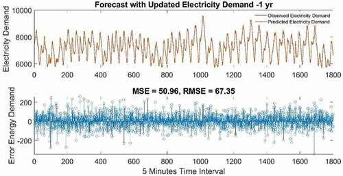
Figure 13. Observed and predicted the highest value for electricity demand

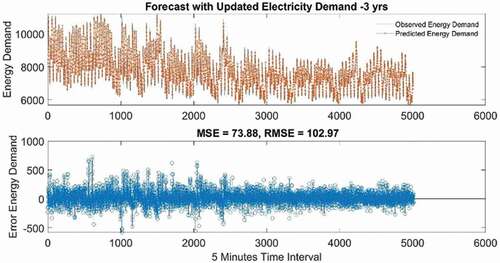
Figure 14. Observed and predicted the highest value for electricity price- one 3 year test dataset

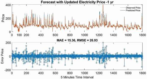
Figure 15. Observed and predicted the highest value for electricity price- 3 year test dataset

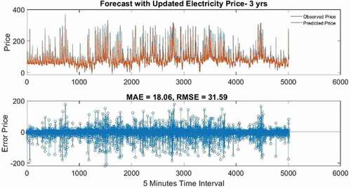
Figure 16. Scatter plot for the electricity demand forecasting models along with the coefficient correlation (R²) in the testing phase corresponding to the (a) 1 year and (b) 3 years dataset

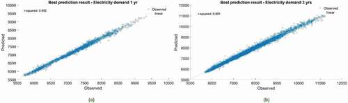
Figure 17. Scatter plot for the electricity price forecasting models along with the coefficient correlation (R²) in the testing phase corresponding to the (a) 1 year and (b) 3 years dataset

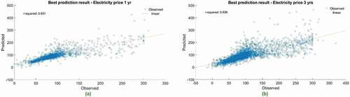
Figure 18. Test error plot for different architectures with and without dropout

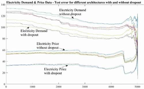
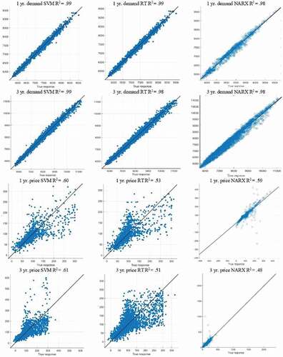
Figure 19. Scatter plot of the compared forecasting models along with the coefficient correlation (R²)

6.1 Test results evaluation

To evaluate the reliability of the proposed LSTM model, the highest observed (actual) value from the test dataset of the electricity demand and price are compared with the forecasted value. The results of the testing process and prediction are summarised in Table 3. Additionally, Table 4 summarises the highest value of electricity demand and price for both data set. Both the highest record for demand and price were on a workday.

Table 4. The highest value of electricity demand and price

	Day and date	Demand	price	Day of the week
3 years data	13/08/2019 19:00	11,221.11	280.4	Workday
	13/08/2019 20:00	10,931.99	369.86	Workday
1 Year data	25/10/2019 16:30	9515	83.09	Workday
	30/10/201,914:30	8199.3	310.87	Workday

The forecasted highest electricity demand occurs at the same time as the observed demand. Whereas, forecasted the highest price occasionally does not fit with actual data. For the 1-year and 3 years electricity demand forecast, the average relative error value of approximately 0.24% and 1.92% respectively, and the highest difference between the relative error values range are 0.36 and 1.1 respectively. Moreover, Figures 14 and 15 indicate that in all cases of forecasted and observed price values of the testing phase, do not demonstrate similarities. However, the average relative error value for the 1 year and 3 years of electricity price forecast is 0.48% and 0.58% respectively, and the highest difference between the relative error values range is 0.83 and 0.89 respectively. This is a reasonable value in the electricity sector given forecasting the highest demand and price. The correct prediction of the highest demand and pricing during peak time and season is difficult, especially when people frequently change their usage patterns in smart city scenarios (Kourtis, Hadjipaschalis, and Poullikkas 2011). Table 6 shows the highest electricity price does not correspond to the highest electricity demand.

The performance evaluation and simulation results of 1 year and 3 years datasets illustrate that the proposed model can produce highly accurate and stable results in both cases. Besides, it also indicates that the proposed LSTM model can produce better forecasting in the absence of a large set of historical datasets. The 1-year dataset is also showing good forecast results.

Several epochs and the hidden units are finalised after several experiments. There is no significant increase in forecasting accuracy after increasing hidden layers (from 250 to 300), as shown in Figures 12–15.

6.2 Ablation study

To investigate the behaviour of the proposed model, this paper has conducted several ablation studies. First, it varies the number of hidden units and epoch in the LSTM networks, as shown in Table 2. Second, to test the robustness of dropout, the same architectures trained without dropout, have drastically different test errors as seen as by the two separate clusters of trajectories in Figure 18. This shows that dropout has a strong regularising effect and gives a huge improvement across all architectures.

6.3 Method comparison

To validate the performance of the proposed LSTM network, some other conventional forecast methods are also performed using the same collected dataset, which includes NARX, SVM, and regression tree (RT). NARX is a recurrent dynamic network, with feedback links that include multiple network layers. The NARX model is used widely in time-

series modelling (Andalib and Atry 2009). The dynamic equation for the NARX model is:

(13) $y\left(t\right)=f\left(y\left(t\right),\left(t-1\right),y\left(t-2\right),\dots ,y\left(t-n_y\right),u\left(t\right),u\left(t-1\right)\dots ,u\left(t-n_u\right)\right)$(13)

where $n$ is the total number of time steps in the input, $y\left(t\right)$ and $u\left(t\right)$ are previous and present independent (exogenous) inputs of the NARX model and $f$ is a nonlinear mapping function. Furthermore, SVM is a supervised learning algorithm, designed to solve non-linear problems and used for regression and classification (Hong et al. 2010). The principle of SVM regression is to consider a nonlinear map from input space to output space for each input parameter vector (x) and its associated output vector (y) and map the data to a higher dimensional feature space through the map. SVM relates the inputs and outputs for the non-linear forecasting model, using:

(14) $y=\mathrm{w}.\phi \left(x\right)+\mathrm{b}$(14)

where w is the weight vector, and b is the bias, which is dependent on the kernel function chosen; in this case, linear, quadratic, cubic, and fine-Gaussian. The kernel function assesses the similarity of the two findings (Walker et al. 2020). $\phi \left(x\right)$ is the nonlinear mapping that is the only hidden space from input space to high–dimensional feature space. RT is a general algorithm for developing statistical tree models that construct a binary tree for regression tasks, which are used for continuous target variables (Tso and Yau 2007).

There are usually two steps to building a regression tree (Walker et al. 2020). During the first step, the set of available predictors values (predictor space x), is divided into J distinct non-overlapping regions $r_1$, $r_2$, …, $r_j$. The regions are designed to ensure that it minimises the residual sum of squares given by (equation. 15)(15) $\sum _{j=1}^J\sum _{i\in r_j}{\left(y_t-{\bar{y}}_{r_j}\right)}^2$(15) . The mean response of the training observations within the $j^{th}$ the region is given by ${\bar{y}}_{r_j}$.

(15) $\sum _{j=1}^J\sum _{i\in r_j}{\left(y_t-{\bar{y}}_{r_j}\right)}^2$(15)

In the second step, for each new occurrence that occurs in a region $r_j$, the prediction gives the mean of the response values for the training observations in $r_j$ (Walker et al. 2020).

Based on the forecast results, the performance of the proposed LSTM network has less error than the compared models as shown in Table 5. The results of the three compared models are also compared in terms of R². The scatter plots of all three models along with their R² values are shown in Figure 19.

Table 5. The performance metrics comparison under different methods

Different Method		RMSE	MAE	R^2
1 year electricity Demand	SVM	79.22	61.40	.99
	RT	84.41	65.37	.99
	NARX	128.72	94.28	.98
	LSTM	67.35	50.96	.99
3 years electricity Demand	SVM	111.97	82.79	.99
	RT	128.3	96.77	.98
	NARX	122.43	91.64	.98
	LSTM	102.50	73.59	.99
1 year electricity Price	SVM	29.91	16.93	.60
	RT	32.29	20.14	.53
	NARX	59	49.77	.59
	LSTM	26.93	15.16	.64
3 years electricity Price	SVM	37.43	19.59	.61
	RT	36.44	22.42	.51
	NARX	52.96	39.12	.48
	LSTM	31.5	18.06	.62

SVM and the proposed LSTM model have the highest R² value of 0.99. This displays a significant correlation between actual and predicted values. Table 5 outlines the best possible results for each model. The findings indicate that the LSTM model being proposed achieves the best results. Compared to SVM, RT, and NARX, the RMSE index of the proposed LSTM model has been averagely improved by 11.25%, 20%, and 33.5% respectively in the case of electricity demand.

Similarly, the MAE has been improved by 14%, 22.5%, and 32.5% respectively. In the case of electricity price, the performance error RMSE shows an improvement of 12.8%, 14.5%, and 47% compared with SVM, RT, and NARX, respectively. Similarly, MAE has been improved by 8.4%, 21%, and 61% respectively.

7. Conclusion

Electricity demand and price Forecasting have important roles in the economy, which is frequently used in business planning, decision making on the supply of electricity, and market setting. Also, this specifies the resource requirements to plan the utility, such as daily natural source usage or integration of RE sources. Therefore, forecasting can benefit the electricity market participants to compete with bidding strategies. However, the literature indicates that electricity demand and price patterns are very complex. It is, therefore, important to develop reliable methods to lessen the uncertainty of forecasting by improving the accuracy.

The results of this paper show LSTM-based sequence-to-sequence network can forecast electricity demand and price for smart city time-series data to achieve good accuracy despite its conceptual simplicity. In contrast to related work, this proposed model first takes electricity demand/price data input sequentially and then output forecast sequentially. This allows handling variable input and output length while simultaneously modelling temporal structure. Additionally, dropout regularisation techniques are used to improve model performance. The feasibility of the proposed LSTM model is confirmed by its performance on well-known real market data of AEMO.

This research used MATLAB as the simulation tool; and RMSE, MAE, and R² as the comparison metrics. Simulation results prove the effectiveness of the proposed method with forecasting in different test cases and granularity. The numerical results show that the LSTM forecasting model has lesser MAE and RMSE. The results indicate that just increasing the number of LSTM layers, which also assess the efficiency of the LSTM model, does not have much impact on the accuracy of the results.

The proposed method has been compared with the SVM, RT, NARX models using the same dataset. The proposed model outperforms other models in all performance indices.

The proposed straightforward model can easily be implemented in real practice. While the findings may be specific to the contexts studied, analytic generalisation could facilitate the application to other types of culture, background and environment. This research work evaluated on a single data set, but further experiments with different datasets are needed to draw more generic conclusions. Future work will also consider other time-series data and explore the universality and reliability features to enhance forecast performance. In future work, to improve the model accuracy, multiple variables such as weather and environmental data, can also be taken into consideration in electricity demand and price forecasting to check model accuracy; and then use feature selection methods to select relevant features although keeping good forecasting accuracy. Besides, this research aims to explore other deep learning algorithms, optimisation models, as well as other regularisation approaches to improve the generalisation of the models.

Disclosure statement

No potential conflict of interest was reported by the author(s).

Additional information

Notes on contributors

Israt Fatema

Israt Fatema received the B.Sc. degree in Information Technology, major in Software Engineering, from the University of Western Sydney (UWS), Australia and the Master of Engineering Studies in Software & Information Systems Engineering from the University of Technology, Sydney (UTS), Australia, and the MPhil degree from IIT, University of Dhaka, Bangladesh. She is currently pursuing a Ph.D. degree with the Faculty of Engineering and Information Technology, School of Electrical and Data Engineering, University of Technology, Sydney (UTS), Australia, where she is also a Researcher and casual academic. Her research interests include smart grid, microgrid, energy trading, optimisation, and forecasting.

Xiaoying Kong

Dr. Xiaoying Kong received her Bachelor of Engineering and Master of Engineering in control engineering from Beijing University of Aeronautics and Astronautics in 1986 and 1989, respectively. She received her Ph.D. degree in mechatronics engineering from the University of Sydney in 2000. She has many years of work experience in the aeronautical industry, semiconductor industry, and software industry. Dr. Kong is currently a senior lecturer at the University of Technology, Sydney. Her research work focuses on two key areas including control engineering and software engineering. She has published research papers broadly on inertial navigation systems, GPS, multi-sensor fusion, indoor navigation, unmanned aircraft navigation, and path planning, traffic flow modelling, agile software development methodologies, and web technologies.

Gengfa Fang

Dr. Gengfa Fang received his Master in Telecommunications from Zhejiang University and Ph.D. in Wireless Communications from the Institute of Computing Technology, Chinese Academy of Sciences in 2002, and 2007 accordingly. From Oct. 2007 to May 2009, he was a Researcher at the Canberra Research Lab of National ICT Australia (NICTA) on the WCDMA Femtocell project. From June 2010 to December 2010, he was working on the Rural Broadband Access project at CSIRO as a Research Scientist. From 2009 to 2015, he was with the Department of Engineering at Macquarie University. In 2016 he moved to UTS where he is now a Senior Lecturer. He has published over 100 papers, patents on embedded wireless network systems, MAC protocols, cross-layer design, wireless resource management, and allocation for 5G, IoT, and Medical Body Area Networks. His research has been supported by CSIRO, NICTA, NXP, Zarlink, Quantenna Communications, and Intel.

References

- Abedinia, O., M. Zareinejad, M. H. Doranehgard, G. Fathi, and N. Ghadimi. 2019. “Optimal Offering and Bidding Strategies of Renewable Energy Based Large Consumer Using a Novel Hybrid Robust- Stochastic Approach.” Journal of Cleaner Production 215: 878–889. doi:https://doi.org/10.1016/J.JCLEPRO.2019.01.085.
- Adhikari, R., and R. K. Agrawal. 2013. “An Introductory Study on Time Series Modeling and Forecasting.” arXiv Preprint arXiv 1302: 6613.
- AEMO report. 2019. Australian Energy Market Operator (AEMO) 2019. Viewed Jan. 2020, https://www.aemo.com.au
- AER Report. 2018. Wholesale Electricity Market Performance Report December 2018. (Australian Energy Regulator). viewed Dec. 2019. https://www.aer.gov.au/wholesale-markets/market-performance/aer-wholesale-electricity-market-performance-report-2018
- Alam, S., and M. Ali. 2020. “Equation Based New Methods for Residential Load Forecasting.” Energies 13 (23): 6378. doi:https://doi.org/10.3390/en13236378.
- Andalib, A., and F. Atry. 2009. “Multi-step Ahead Forecasts for Electricity Prices Using NARX: A New Approach, a Critical Analysis of One-step Ahead Forecasts.” Energy Conversion and Management 50 (3): 739–747. doi:https://doi.org/10.1016/j.enconman.2008.09.040.
- Bouktif, S., A. Fiaz, A. Ouni, and M. A. Serhani. 2018. “Optimal Deep Learning Lstm Model for Electric Load Forecasting Using Feature Selection and Genetic Algorithm: Comparison with Machine Learning Approaches.” Energies 11 (7): 1636. doi:https://doi.org/10.3390/en11071636.
- Brownlee, J. 2018. Deep learning for time series forecasting: predict the future with MLPs, CNNs and LSTMs in Python, Machine Learning Mastery.
- Chen, B.-J., M.-W. Chang, and C.-J. Lin. 2004. “Load Forecasting Using Support Vector Machines: A Study on EUNITE Competition 2001.” IEEE Transactions on Power Systems 19 (4): 1821–1830. doi:https://doi.org/10.1109/TPWRS.2004.835679.
- Dehalwar, V., A. Kalam, M. L. Kolhe, and A. Zayegh. 2016. “Electricity Load Forecasting for Urban Area Using Weather Forecast Information.” In 2016 IEEE International Conference on Power and Renewable Energy (ICPRE), Shanghai, China, 355–359. IEEE. doi:https://doi.org/10.1109/ICPRE.2016.7871231.
- Ertugrul, Ö. F. 2016. “Forecasting Electricity Load by a Novel Recurrent Extreme Learning Machines Approach.” International Journal of Electrical Power & Energy Systems 78: 429–435. doi:https://doi.org/10.1016/j.ijepes.2015.12.006.
- Gao, W., A. Darvishan, M. Toghani, M. Mohammadi, O. Abedinia, and N. Ghadimi. 2019. “Different States of Multi-block Based Forecast Engine for Price and Load Prediction.” International Journal of Electrical Power & Energy Systems 104: 423–435. doi:https://doi.org/10.1016/j.ijepes.2018.07.014.
- Garreta, R., and G. Moncecchi. 2013. Learning Scikit-learn: Machine Learning in Python. Birmingham: Packt Publishing .
- Ghadimi, N., A. Akbarimajd, H. Shayeghi, and O. Abedinia. 2018. “Two Stage Forecast Engine with Feature Selection Technique and Improved Meta-heuristic Algorithm for Electricity Load Forecasting.” Energy 161: 130–142. doi:https://doi.org/10.1016/j.energy.2018.07.088.
- Ghasemi, A., H. Shayeghi, M. Moradzadeh, and M. Nooshyar. 2016. “A Novel Hybrid Algorithm for Electricity Price and Load Forecasting in Smart Grids with Demand-side Management.” Applied Energy 177: 40–59. doi:https://doi.org/10.1016/j.apenergy.2016.05.083.
- Gong, G., X. An, N. K. Mahato, S. Sun, S. Chen, and Y. Wen. 2019. “Research on Short-term Load Prediction Based on Seq2seq Model.” Energies 12 (16): 3199. doi:https://doi.org/10.3390/en12163199.
- Graves, A., A.-R. Mohamed, and G. Hinton. 2013. “Speech Recognition with Deep Recurrent Neural Networks.” In 2013 IEEE International Conference on Acoustics, Speech and Signal Processing, Vancouver, BC, Canada, 6645–6649. IEEE. doi:https://doi.org/10.1109/ICASSP.2013.6638947.
- Hochreiter, S., and J. Schmidhuber. 1997a. “Long Short-term Memory.” Neural Computation 9 (8): 1735–1780. doi:https://doi.org/10.1162/neco.1997.9.8.1735.
- Hochreiter, S., and J. Schmidhuber. 1997b. “LSTM Can Solve Hard Long Time Lag Problems.” Advances in Neural Information Processing Systems, Denver, CO, USA, Denver, CO, USA, 2–5 December 2–5, 1996, 473–479.
- Hong, T., M. Gui, M. E. Baran, and H. L. Willis. 2010. “Modeling and Forecasting Hourly Electric Load by Multiple Linear Regression with Interactions.” IEEE PES General Meeting 1–8. IEEE. doi:https://doi.org/10.1109/PES.2010.5589959.
- Hu, M. Y., G. Zhang, C. X. Jiang, and B. E. Patuwo. 1999. “A Cross-validation Analysis of Neural Network Out-of-sample Performance in Exchange Rate Forecasting.” Decision Sciences 30 (1): 197–216. doi:https://doi.org/10.1111/j.1540-5915.1999.tb01606.x.
- Jabir, H. J., J. Teh, D. Ishak, and H. Abunima. 2018. “Impacts of Demand-side Management on Electrical Power Systems: A Review.” Energies 11 (5): 1050. doi:https://doi.org/10.3390/en11051050.
- Jiang, P., F. Liu, and Y. Song. 2017. “A Hybrid Forecasting Model Based on Date-framework Strategy and Improved Feature Selection Technology for Short-term Load Forecasting.” Energy 119: 694–709. doi:https://doi.org/10.1016/j.energy.2016.11.034.
- Khodaei, H., M. Hajiali, A. Darvishan, M. Sepehr, and N. Ghadimi. 2018. “Fuzzy-based Heat and Power Hub Models for Cost-emission Operation of an Industrial Consumer Using Compromise Programming.” Applied Thermal Engineering 137: 395–405. doi:https://doi.org/10.1016/j.applthermaleng.2018.04.008.
- Khuntia, S. R., J. L. Rueda, and M. A. Van der Meijden. 2018. “Long-term Electricity Load Forecasting considering Volatility Using Multiplicative Error Model.” Energies 11 (12): 3308. doi:https://doi.org/10.3390/en11123308.
- Kourtis, G., I. Hadjipaschalis, and A. Poullikkas. 2011. “An Overview of Load Demand and Price Forecasting Methodologies.” International Journal of Energy & Environment 2 (1): 123-150.
- Kuo, P.-H., and C.-J. Huang. 2018. “An Electricity Price Forecasting Model by Hybrid Structured Deep Neural Networks.” Sustainability 10 (4): 1280. doi:https://doi.org/10.3390/su10041280.
- Lau, E., L. Sun, and Q. Yang. 2019. “Modelling, Prediction and Classification of Student Academic Performance Using Artificial Neural Networks.” SN Applied Sciences 1 (9): 1–10. doi:https://doi.org/10.1007/s42452-019-0884-7.
- Le, X.-H., H. V. Ho, G. Lee, and S. Jung. 2019. “Application of Long Short-term Memory (LSTM) Neural Network for Flood Forecasting.” Water 11 (7): 1387. doi:https://doi.org/10.3390/w11071387.
- LeCun, Y., Y. Bengio, and G. Hinton. 2015. “Deep Learning.” nature 521 (7553): 436–444. doi:https://doi.org/10.1038/nature14539.
- Li, C., Z. Ding, D. Zhao, J. Yi, and G. Zhang. 2017. “Building Energy Consumption Prediction: An Extreme Deep Learning Approach.” Energies 10 (10): 1525. doi:https://doi.org/10.3390/en10101525.
- Li, K., and T. Zhang. 2018. “Forecasting Electricity Consumption Using an Improved Grey Prediction Model.” Information 9 (8): 204. doi:https://doi.org/10.3390/info9080204.
- Lipton, Z. C., J. Berkowitz, and C. Elkan. 2015. “A Critical Review of Recurrent Neural Networks for Sequence Learning.” arXiv Preprint arXiv:1506.00019.
- Marino, D. L., K. Amarasinghe, and M. Manic 2016. “Building Energy Load Forecasting Using Deep Neural Networks.” IECON 2016–42nd Annual Conference of the IEEE Industrial Electronics Society, IEEE, Florence, Italy, October 23–26, 2016, pp. 7046–7051. doi: https://doi.org/10.1109/IECON.2016.7793413.
- Medennikov, I., and A. Bulusheva 2016. “LSTM-based Language Models for Spontaneous Speech Recognition.” International Conference on Speech and Computer, Budapest, Hungary, August 23-27, 2016, Springer, pp. 469–475. doi: https://doi.org/10.1007/978-3-319-43958-7_56.
- Mikolov, T., A. Joulin, S. Chopra, M. Mathieu, and M. A. Ranzato. 2014. “Learning Longer Memory in Recurrent Neural Networks.” arXiv Preprint arXiv:1412.7753.
- Mohandes, M. 2002. “Support Vector Machines for Short-term Electrical Load Forecasting.” International Journal of Energy Research 26 (4): 335–345. doi:https://doi.org/10.1002/er.787.
- Mujeeb, S., N. Javaid, M. Akbar, R. Khalid, O. Nazeer, and M. Khan 2018. “Big Data Analytics for Price and Load Forecasting in Smart Grids.” International Conference on Broadband and Wireless Computing, Communication and Applications, Switzerland, Springer, pp. 77–87. doi: https://doi.org/10.1007/978-3-030-02613-4_7.
- Mujeeb, S., N. Javaid, M. Ilahi, Z. Wadud, F. Ishmanov, and M. K. Afzal. 2019. “Deep Long Short-term Memory: A New Price and Load Forecasting Scheme for Big Data in Smart Cities.” Sustainability 11 (4): 987. doi:https://doi.org/10.3390/su11040987.
- Nagbe, K., J. Cugliari, and J. Jacques. 2018. “Short-term Electricity Demand Forecasting Using a Functional State Space Model.” Energies 11 (5): 1120. doi:https://doi.org/10.3390/en11051120.
- Nelson, D. M., A. C. Pereira, and R. A. de Oliveira 2017. “Stock Market’s Price Movement Prediction with LSTM Neural Networks.” 2017 International joint conference on neural networks (IJCNN), Anchorage, AK, USA, May 14–19, 2017, IEEE, pp. 1419–1426. doi: https://doi.org/10.1109/IJCNN.2017.7966019.
- Pan, L., X. Feng, F. Sang, L. Li, M. Leng, and X. Chen. 2019. “An Improved Back Propagation Neural Network Based on Complexity Decomposition Technology and Modified Flower Pollination Optimization for Short-term Load Forecasting.” Neural Computing and Applications 31 (7): 2679–2697. doi:https://doi.org/10.1007/s00521-017-3222-2.
- Papalexopoulos, A. D., and T. C. Hesterberg. 1990. “A Regression-based Approach to Short-term System Load Forecasting.” IEEE Transactions on Power Systems 5 (4): 1535–1547. doi:https://doi.org/10.1109/PICA.1989.39025.
- Park, D. C., El-Sharkawi, M. A., Marks, R. J., Atlas, L., and M. Damborg. 1991. “Electric load forecasting using an artificial neural network.” https://doi.org/10.1109/59.76685.
- Roldán-Blay, C., G. Escrivá-Escrivá, C. Álvarez-Bel, C. Roldán-Porta, and J. Rodríguez-García. 2013. “Upgrade of an Artificial Neural Network Prediction Method for Electrical Consumption Forecasting Using an Hourly Temperature Curve Model.” Energy and Buildings 60: 38–46. doi:https://doi.org/10.1016/j.enbuild.2012.12.009.
- Saeedi, M., M. Moradi, M. Hosseini, A. Emamifar, and N. Ghadimi. 2019. “Robust Optimization Based Optimal Chiller Loading under Cooling Demand Uncertainty.” Applied Thermal Engineering 148: 1081–1091. doi:https://doi.org/10.1016/j.applthermaleng.2018.11.122.
- Sehovac, L., and K. Grolinger. 2020. “Deep Learning for Load Forecasting: Sequence to Sequence Recurrent Neural Networks with Attention.” IEEE Access 8: 36411–36426. doi:https://doi.org/10.1109/ACCESS.2020.2975738.
- Srivastava, N., G. Hinton, A. Krizhevsky, I. Sutskever, and R. Salakhutdinov. 2014. “Dropout: A Simple Way to Prevent Neural Networks from Overfitting.” The Journal of Machine Learning Research 15 (1): 1929–1958.
- Suganthi, L., S. Iniyan, and A. A. Samuel. 2015. “Applications of Fuzzy Logic in Renewable Energy Systems–a Review.” Renewable and Sustainable Energy Reviews 48: 585–607. doi:https://doi.org/10.1016/j.rser.2015.04.037.
- Sutskever, I., O. Vinyals, and Q. V. Le. 2014. “Sequence to Sequence Learning with Neural Networks.” Advances in Neural Information Processing Systems, Montreal, Canada, December 8 – 13, 2014, 3104–3112.
- Szkuta, B., L. A. Sanabria, and T. S. Dillon. 1999. “Electricity Price Short-term Forecasting Using Artificial Neural Networks.” IEEE Transactions on Power Systems 14 (3): 851–857. doi:https://doi.org/10.1109/59.780895.
- Tong, C., J. Li, C. Lang, F. Kong, J. Niu, and J. J. Rodrigues. 2018. “An Efficient Deep Model for Day-ahead Electricity Load Forecasting with Stacked Denoising Auto-encoders.” Journal of Parallel and Distributed Computing 117: 267–273. doi:https://doi.org/10.1016/j.jpdc.2017.06.007.
- Tso, G. K., and K. K. Yau. 2007. “Predicting Electricity Energy Consumption: A Comparison of Regression Analysis, Decision Tree and Neural Networks.” Energy 32 (9): 1761–1768. doi:https://doi.org/10.1016/j.energy.2006.11.010.
- Ugurlu, U., I. Oksuz, and O. Tas. 2018. “Electricity Price Forecasting Using Recurrent Neural Networks.” Energies 11 (5): 1255. doi:https://doi.org/10.3390/en11051255.
- Walker, S., W. Khan, K. Katic, W. Maassen, and W. Zeiler. 2020. “Accuracy of Different Machine Learning Algorithms and Added-value of Predicting Aggregated-level Energy Performance of Commercial Buildings.” Energy and Buildings 209: 109705. doi:https://doi.org/10.1016/j.enbuild.2019.109705.
- Wan, L., M. Zeiler, S. Zhang, Y. Le Cun, and R. Fergus 2013. “Regularization of Neural Networks Using Dropconnect.” International conference on machine learning, Atlanta, USA, June 16 – 21, 2013, pp. 1058–1066.
- Wang, F., K. Li, L. Zhou, H. Ren, J. Contreras, M. Shafie-Khah, and J. P. Catalão. 2019. “Daily Pattern Prediction Based Classification Modeling Approach for Day-ahead Electricity Price Forecasting.” International Journal of Electrical Power & Energy Systems 105: 529–540. doi:https://doi.org/10.1016/j.ijepes.2018.08.039.
- Wang, J., F. Liu, Y. Song, and J. Zhao. 2016. “A Novel Model: Dynamic Choice Artificial Neural Network (DCANN) for an Electricity Price Forecasting System.” Applied Soft Computing 48: 281–297. doi:https://doi.org/10.1016/j.asoc.2016.07.011.
- Wang, K., C. Xu, Y. Zhang, S. Guo, and A. Y. Zomaya. 2017. “Robust Big Data Analytics for Electricity Price Forecasting in the Smart Grid.” IEEE Transactions on Big Data 5 (1): 34–45. doi:https://doi.org/10.1109/TBDATA.2017.2723563.
- Wang, K., X. Qi, and H. Liu. 2019. “Photovoltaic Power Forecasting Based LSTM-Convolutional Network.” Energy 189: 116225. doi:https://doi.org/10.1016/j.energy.2019.116225.
- Xu, L., C. Li, X. Xie, and G. Zhang. 2018. “Long-short-term Memory Network Based Hybrid Model for Short-term Electrical Load Forecasting.” Information 9 (7): 165. doi:https://doi.org/10.3390/info9070165.
- Yu, M., and S. H. Hong. 2016. “Supply–demand Balancing for Power Management in Smart Grid: A Stackelberg Game Approach.” Applied Energy 164: 702–710. doi:https://doi.org/10.1016/j.apenergy.2015.12.039.
- Yue, H., L. Dan, and G. Liqun 2012. “Power System Short-term Load Forecasting Based on Neural Network with Artificial Immune Algorithm.” 2012 24th Chinese Control and Decision Conference (CCDC), Taiyuan, China, May 23–25, 2012, IEEE, pp. 844–848. doi: https://doi.org/10.1109/CCDC.2012.6244131.
- Zahid, M., F. Ahmed, N. Javaid, R. A. Abbasi, H. S. Zainab Kazmi, A. Javaid, M. Bilal, M. Akbar, and M. Ilahi. 2019. “Electricity Price and Load Forecasting Using Enhanced Convolutional Neural Network and Enhanced Support Vector Regression in Smart Grids.” Electronics 8 (2): 122. doi:https://doi.org/10.3390/electronics8020122.
- Zaytar, M. A., and C. El Amrani. 2016. “Sequence to Sequence Weather Forecasting with Long Short-term Memory Recurrent Neural Networks.” International Journal of Computer Applications 143 (11): 7–11. doi:https://doi.org/10.5120/ijca2016910497.
- Zhang, R., Z. Y. Dong, Y. Xu, K. Meng, and K. P. Wong. 2013. “Short-term Load Forecasting of Australian National Electricity Market by an Ensemble Model of Extreme Learniweang Machine.” IET Generation, Transmission & Distribution 7 (4): 391–397. doi:https://doi.org/10.1049/iet-gtd.2012.0541.