Consignment stock management for reducing waste items and GHG emissions using remanufacturing, emission penalties and promotional efforts under capacity constraints

ABSTRACT

Most business organizations aim is to make as much profit as possible. In this consignment stock model, we discuss the reworking of waste items and reductions of greenhouse gases (GHGs). Here, we determine the GHGs and GHG penalty costs for each manufacturing and remanufacturing lot size. This proposed model is developed to reduce the manufacturer’s total cost per unit time without shortages. Also, we introduced a warehouse capacity constraint (CC) for minimizing the holding cost. For the promotional efforts, retailer promotional activity becomes prevalent in the business world, and here the promotional efforts dependent on demand. We exhibit the numerical instance by performing a sensitivity analysis of the model parameters and discussing specific managerial insights using optimization techniques.

KEYWORDS:

• Remanufacturing
• GHGs
• Penalty cost
• Capacity Constraints
• Promotional Effort

1. Introduction

In this paper, we discuss the fundamental responsibilities of consignment stock management (CSM) to reduce waste items and GHGs by using reworking/remanufacturing. CSM allows a seller (manufacturer) to place merchandise in wholesale and retail outlets for buying market. It can provide an incentive for the wholesaler and retailer to stock goods in inventory. Also, it provides the manufacturer with an opportunity to have merchandise exposed to the buying market instead of having it stored and isolated in a warehouse while waiting for an order from a buyer. The role of promotional effort is most beneficial to minimize the cost, which is dependent on demand. Generally, promotional policies include gifts, price discounts, displays, permissible delay in payment. It is an essential factor so that it is impossible to ignore the impact of promotional effort in the inventory controls. A consignment sale is an agreement in which a third party is entrusted with selling goods on behalf of the owner. This study offers two kinds of shops; the first shop (serviceable stock) manufactures new products and remanufactures used ones accumulated from waste items through the second shop (repairable stock). The following elements are considered to be efficient strategies in this model. It is the method of changing waste materials into new materials, storing material, and reducing GHGs. Recycling can prevent the waste of potentially useful materials and reduce the consumption of sparkling raw materials. Recycling is a key factor in modern waste reduction and has some basic principles: Reduce, Reuse and Recycle (3R). It is mass communication for maximizing the company’s profits and minimizing cost. Sales advertising is undertaken for a wide variety of purposes, including promoting a new product, air pollution control, exclusive achievements of employees, Publicizing new policies or an extension in sales. The promotional efforts are personal selling, direct marketing, advertising, public relations, sponsorship, sales promotion, permissible delay in payments and digitalization. On the other side, the GHGs trap heat and make the planet warmer. The largest source of GHGs from human activities from burning fossil fuels for electricity, heat, and transportation. GHGs is a gaseous compound in the atmosphere that is successful in absorbing infrared radiation. By growing the heat in the atmosphere, the GHGs are responsible for their effect and leading to global warming. GHGs will be reduced if the authorities judge the GHG penalty costs for the companies and transport users. The elements of the sources of GHGs are power plants, residential and industrial buildings, road transports, forest degradation, electricity industry process, cement and ceramics production, livestock, iron and steel production, agricultural soil, chemical and petrochemical industries, oil and gasoline production, waste items, coal mining, aviation. This CSM involves two different warehouse constraints: owned warehouse (OW) while the other is a rented warehouse (RW). The RW is used to store units over the fixed capacity (Cow$C_{ow}$) of the owned warehouse, and these factors may suggest retailers buy more than their OW capacity. In these situations, the retailers can benefit from a rented warehouse (RW).

1.1. Framework of the paper

The rest of this paper can be described as follows: (Section 2) and (Section 3) refers to the relevant literature and basic mathematical notations. The assumptions and development of the cost functions are presented in Section 6 and Section 7. Section 8 and Section 9 presents the numerical examples and sensitivity analysis to facilitate a general understanding of the CSM system, managerial insights, and the key factors used to extend the discussion beyond the results of this paper. Finally, we conclude this research in Section 10.

2. Literature review

From this literature review, we have some basic ideas to minimize the total cost and optimizing the decision variables of manufacturing and remanufacturing. The following literature summary gives more responsibilities to this model.

Consignment stock

In 2020, Chen et.al (Chen and Su 2020) implemented a consignment supply chain (SC) cooperation for complementary products under online to offline business mode. From Glock’s (Glock 2012) lot-size model, we optimize the lot-sizes for production and reworking. Hemmati et.al (Hemmati, Fatemi Ghomi, and Sajadieh 2017) analyzed the importance of VMI and CSM for a SC. In 2016, Jaber et.al (Jaber, Bazan, and Zanoni 2016) reviewed the benifits of transportation and logistics. Lee et.al (Lee, Wang, and Chen 2017) addressed the forward and backward stocking policies for a two-level SC with consignment agreement and stock-dependent demand. The major problem in an inventory is to minimize the cost which is overcome by Sha et.al (Shah, Shah, and Patel 2015) since, they discussed about the use of retailers price policies under trended demand.

Remanufacturing

The high populations and rapid urbanization affect the environment by waste items. In 2013, Jaber et.al (Hasanov et al. 2013) developed the method for reducing the waste items with disposal and transportation costs in a closed-loop SC model. For this model, the work of CSM is necessary for disposing of the waste items by remanufacturing, which is discussed by Jaber et.al (Jaber, Zanoni, and Zavanella 2014). If the sales are lost then, the manufacturer can manage the problem to sell the reworked items. In 2020, Ndhaief et.al (Ndhaief et al. 2020) investigated an integrated production and maintenance control of unreliable production/rework systems. In 2019, Taleizadeh et.al (Taleizadeh, Alizadeh-Basban, and Niaki 2019) constructed a closed-loop SC with carbon reduction, quality improvement effort, and return policy under two rework scenarios.

Promotional efforts

In a digital world, advertisement is essential for every commercial industry or organization.

• Advertising helps for increasing the sales.

• Advertising helps producers or companies to understand their competitors.

• If any company needs to introduce or launch a new product in the market, advertising will make a floor for the product.

• The demand for the product keeps coming with the help of advertising, and supply comes to be a never-ending process.

In 2019, Ebrahimi et.al (Ebrahimi, Hosseini-Motlagh, and Nematollahi 2019) developed a model for the delay in payment contract for coordinating a two-echelon periodic review SC with stochastic promotional effort dependent demand. In 2014, Maihami et.al (Maihami and Karimi 2014) addressed the replenishment policy for non-instantaneous deteriorating items with stochastic demand and promotional efforts. For minimizing the total cost by promotional efforts, we consider the Palanivel and Uthayakumar’s (Palanivel and Uthayakumar 2017) production-inventory model with promotional effort, variable production cost, and probabilistic deterioration. Furthermore, Malleeswaran and Uthayakumar (2020) illustrated an integrated inventory model with backorder price discounts and price-dependent demand under service level constraints.

Green house gases (GHGs)

Transport is a crucial avenue to reduce GHGs, and any substantial effort to reduce GHGs will need to inspire towards more fuel-efficient, less polluting behaviour. Many researchers discussed how to reduce GHGs with GHG penalty costs. In 2014, Bozorgi et.al (Bozorgi, Pazour, and Nazzal 2014) presented an inventory model for cold items with emissions. The effect of GHG in the environment is high. In 2019, Ganesh Kumar and Uthayakumar (Ganesh Kumar and Uthayakumar 2019) developed the mathematical solutions of VMI policies with equal and unequal shipments under GHGs trading to reduce of GHGs. In 2020, (Ghosh 2020) Ghosh introduced an optimization for a production-inventory model with a hybrid carbon policy under random demand. Hertwich et al. (Hertwich et al. 2019) implemented the efficient strategies to reducing GHGs with buildings, vehicles, and electronics a review. For any inventory management, the process of SC is a must. In 2013, Jaber et.al (Jaber, Glock, and El Saadany 2013) described an inventory model for reducing GHGs with SC coordinates. The problem of GHGs is not only in transportations, which also may include waste items. For this issue, Jaber et al. (Jaber, Bazan, and El Saadany 2015) introduced an inventory model for carbon emissions (CEs) in waste items with production and reworking process. The reduction of CEs in transportation and inventory management:(R, Q) policy is developed by Tang et al. (Tang et al. 2018). In 2018, Tiwari et al. (Tiwari, Daryanto, and Wee 2018) studied an inventory model for deteriorating and imperfect quality items with CEs. In 2014, Zanoni et al. (Zanoni, Mazzoldi, and Jaber 2014) discussed the merits in the single vendor-buyer problem under the GHGs.

Capacity constraints (CC)

In 2012, Chao et al. (Chao, Yang, and Yifan 2012) developed the dynamical inventory model for fixed ordering cost in a capacitated stochastic inventory. Lee et al. (Lee, Wang, and Chang 2012) discussed the inventory model for a deteriorating item while the buyer has warehouse CC. In 2010, Liao and Hung (Liao and Huang 2010) developed the deterministic inventory model for deteriorating items with trade credit financing under the CC. The involvement of EOQ is necessary for the inventory model. In 2020, Rezagholifam et al. (Rezagholifam et al. 2020) identified optimal pricing and ordering strategy for non-instantaneous deteriorating items with price and stock sensitive demand and CC. In 2015, Sana (Sana 2015) introduced an EOQ model for the limited capacity of owned warehouses under stochastic demand. Williams et al. (Williams, Ghiami, and Wu 2013) discussed the two-echelon inventory model for a deteriorating item with stock-dependent demand, partial backlogging, and CC. In this section, we discussed the important literature on promotional efforts, warehouse constraints, and GHGs to create an environment without pollutions. This proposed model is seen as a preliminary step for developing an environmentally responsible closed-loop reverse SC model.

2.1. Problem description

The major problem is to reduce the pollution in the global. Humans and companies need to learn the 5 R’s to reduce the GHGs and waste items by refusing, reducing, reuse, rot, recycling, conserve water, and switching to sustainable clean energy. This research provides a clear understanding of the current state of global CEs research and possible future research directions. The study will serve as an update and helpful reference for practitioners and policymakers to prepare for their future work. Moreover, our study aims to identify the area(s) in which a business can effectively reduce costs and maximize profits.

2.2. Research questions?

1. What are the key factors in reducing the waste items and GHGs during the production, transportation, and delivery time under a CSM?

2. What strategies will be used to reduce the waste items and GHGs if the expected demand depends on the promotional effort?

3. What kind of changes will occur in the total cost function if the holding costs depend on the CC?

3. Notations

3.1. Decision variables

Table

$Q_{mls}$ Manufacturing lot-size
$R_{rls}$ Remanufacturing lot-size
$n$ Number of manufacturing batches per cycle
$m$ Number of remanufacturing batches per cycle

3.2 Parameters

3.2.1. Manufacturing and remanufacturing

Table

$w_d$ Number of waste items (waste/year)
$C_w$ Cost for disposing wastes per year ($/unit)
$S_c^m$ Setup cost for manufacturing ($/setup)
$S_c^r$ Setup cost for remanufacturing ($/setup)
${\delta }_{mr}$ Manufacturing rate per unit (units/year)
${\delta }_{rr}$ Remanufacturing rate per unit (units/year)
$M_c^w$ Manufacturing cost per unit (units/year)
$R_c^w$ Remanufacturing cost per unit (units/year)
$h_{rrs}$ Holding cost for a returned unit of repairable stock
where, $h_{mss}>h_{rss}$ and $h_{rss}>h_{rrs}$ (units/year)
$h_{mss}$ Holding cost for a manufactured unit of serviceable stock (units/year)
$h_{rss}$ Holding cost for a remanufactured unit of serviceable stock
where, $h_{mss}\ne h_{rss}$ (units/year)

3.2.2 GHGs and penalty

Table

$E_c^w$ Cost of energy [/KWh]$/KWh]$

$GH{G}_{ER}$ GHGs for rework (ton/unit)

$GH{G}_{EM}$ GHGs for production (ton/unit)

$GH{G}_{cet}$ CEs tax per ton of GHGs ($/ton)

$E_{p{c}_j}$ Emission penalty cost for rework

$E_{p{c}_i}$Emission penalty cost for production

$E_{M{L}_i}$ Manufacturing emission limit $i$ (ton/year)

$E_{R{L}_j}$ Remanufacturing emission limit $j$ (ton/year)

$r_1,r_2,r_3$ Emission function parameters for rework

$m_1,m_2,m_3$ Emission function parameters for production

$Cm$ & $Cr$ Coefficient of the inverse model (required energy

at the machine to production and rework is one unit), [kWh/unit]

$Cm\prime$ & $Cr\prime$ Coefficient of the predictor (required energy per year when production

and rework is idle), [KWh/year]

$GH{G}_{gt}$ Number of gallons per truck per distance travelled, [gallons/truck]

$GH{G}_{et}$ Amount of GHGs from one gallon of diesel-truck fuel, [ton/gallon]

${\mathrm{\Phi }}_M$, ${\mathrm{\Phi }}_R$ Manufacturing and Remanufacturing emissions limit variable functions.

For emissions limits $i$, $j$, which is $1$ if the emissions exceed the allowable

limits $i$ and $j$, $0$ otherwise

3.2.3 Promotional efforts

Table

$\rho$ Promotional effort ($/unit)

$PE{C}^w$ Promotional Effort Cost

${\theta }_k$ Constant terms $>0$, for $k=1,2,3,4,5$ ($/unit)

$D(S_{P_w},t)$ Rate of demand, where, $D(S_{P_w},t)=({\theta }_1-{\theta }_2{S}_{P_w})e^{{\theta }_4}t$

3.2.4 Capacity constriant

Table

$C_{ow}$ Capacity of OW ($/unit)

$t_c^w$ Truck capacity, [units/truck]

$C_F^w$ Fixed cost per truck per trip, [$/truck]

$I_{OW}(t)$ Inventory level at time $t\in (0,{\pi }_0)$ in OW

$I_{RW}(t)$ Inventory level at time $t\in (0,{\pi }_1)$ in RW

${\alpha }_{ow}$ Cost for waste items transported to OW $(0<{\alpha }_{ow}<1)$ ($/unit)

${\alpha }_{rw}$ Cost for waste items transported to RW $({\alpha }_{rw}>{\alpha }_{ow})$ ($/unit)

$t_k^w$ Number of trucks required per year, where $t_k^w=\frac{D(S_{P_w},t)}{t_c^w}$

3.2.5 General

Table

$S_{P_w}$ Selling price ($/unit)

$P_{C_w}$ Purchasing cost ($/unit)

${\mu }_t$ Cycle time for an interval of the total inventory

${\pi }_1$ Length of the interval of RW and ${\pi }_1<{\pi }_0$

${\pi }_0$ Length of the interval of OW and $0<{\pi }_0<\pi <1$

$\pi$ Length of the interval for total inventory system, $0<\pi <1$

${\eta }_1$ Nominal proportion of items returned for remanufacturing when an item is

remanufactured for an unlimited number of times. where, $0<{\eta }_1<1$ ($/unit)

${\eta }_2$ Actual proportion of items returned for recovery purposes when an item is

recovered for a limited number of times ($/unit)

3.2.6 Cost functions

Table

$ATEC$ Annual Total Expected Cost

$ATE{C}^w$ $ATEC$ without CC

$ATE{C}_{ow}^w$ $ATEC$ with Owned Warehouse (OW)

$ATE{C}_{rw}^w$ $ATEC$ with Rented Warehouse (RW)

${ }^{†}$ Denotes the optimal minimum costs of $ATE{C}^w$, $ATE{C}_{ow}^w$, and $ATE{C}_{rw}^w$.

4. Assumptions

The following assumptions are used to develop our model.

4.1. Remanufacturing

1. The total cycle time (${\mu }_t$) can be calculated from the waste items and the manufacturing lot size with respect to demand.

(1) $\mathrm{T}\mathrm{h}\mathrm{a}\mathrm{t}\mathrm{i}\mathrm{s},{\mu }_t=\frac{n{Q}_{mls}(w_d+{\eta }_2)}{w_{d}D(S_{P_w},t)}$(1)

2. The purpose of remanufacturing is the proportion of items returned for recovery purposes when an item is recovered for a limited number $({\eta }_2)$ of times.

$\mathrm{w}\mathrm{h}\mathrm{e}\mathrm{r}\mathrm{e},{\eta }_2=1-\left(\frac{1-{\eta }_1}{w_d}\right)$

3. The number of lot-sizes for the remanufacturing is,

(2) $R_{rls}=C_w\lambda$(2)

$\mathrm{w}\mathrm{h}\mathrm{e}\mathrm{r}\mathrm{e},\lambda =\frac{{\eta }_{2}n{Q}_{mls}}{w_{d}m}$

4.2. GHG penalty

4.2.1. Manufacturing

The role of GHG penalty cost is useful to reduce the pollutions.

(3) ${\mathrm{\Phi }}_M=\left\{\begin{array}{cc}1& ifD(S_{P_w},t)GH{G}_{EM}>E_{M_i}\\ 0& else\end{array}\right.$(3)

where,

$GH{G}_{EM}=m_1{\delta }_{mr}^2-m_2{\delta }_{mr}+m_3$

.

4.2.2. Remanufacturing

(4) ${\mathrm{\Phi }}_R=\left\{\begin{array}{cc}1& ifD(S_{P_w},t)GH{G}_{ER}>E_{R_j}\\ 0& else\end{array}\right.$(4)

where,

$GH{G}_{ER}=r_1{\delta }_{rr}^2-r_2{\delta }_{rr}+r_3$

.

4.3. Promotional efforts

The work of promotional effort is to sell waste items by using remanufacturing. In this proposed model, we give the promotional effort dependent demand, which is exponentially distributed w.r.t. the selling price and cost of transported items to the warehouses.

(5) $\mathrm{T}\mathrm{h}\mathrm{a}\mathrm{t}\mathrm{i}\mathrm{s},PE{C}^w=K(\rho -1{)}^2{\left\{{\int }_0^{\pi }D(S_{P_w},t)e^{{\theta }_{4}t}dt\right\}}^{{\theta }_5}$(5)

From Eqn.(5(5) $\mathrm{T}\mathrm{h}\mathrm{a}\mathrm{t}\mathrm{i}\mathrm{s},PE{C}^w=K(\rho -1{)}^2{\left\{{\int }_0^{\pi }D(S_{P_w},t)e^{{\theta }_{4}t}dt\right\}}^{{\theta }_5}$(5) ), $K=\frac{{\theta }_3}{nm}$ and the basic demand rate is linearly decreasing function of the price and increases exponentially with time when ${\theta }_4>0$ and $\rho \ne 1$.

where,

$D(S_{P_w},t)=({\theta }_1-{\theta }_2{S}_{P_w})e^{{\theta }_4}t$

4.4. Capacity Constraints (CC)

The responsibility of CC in this proposed model is to reduce the holding and total system cost. Let $I_{OW}(t)$ denotes the inventory level at time ${\pi }_0\in (0,\pi )$ in OW, in which the inventory level is decreasing only owing to disposal of the waste item. $I_{RW}(t)$ denote the inventory level at time ${\pi }_1\in (0,\pi )$ in RW, in which the inventory level is decreasing to zero due to demand and disposal of the waste items, where $0<{\pi }_0<\pi <1$. For this warehouse constraint, we classify two kinds of warehouses as owned and rented warehouses respectively.

1. If $Q_{mls},R_{rls}\le C_{ow}$

The production and rework lot-sizes $Q_{mls}$ and $R_{rls}$ is less than or equal to the capacity of the owned warehouse $C_{ow}$ then, the behaviour of OW can be represented by the following differential equation (DE).

(6) $\frac{d{I}_{OW}(t)}{dt}=-({\alpha }_{ow}{I}_{OW}(t)+D(S_{P_w},t))$(6)

with boundary condition, $I_{OW}(\pi )=0$ and $(0<{\alpha }_{ow}<1)$.

2. If $Q_{mls},R_{rls}>C_{ow}$

The production and rework lot-sizes $Q_{mls}$ and $R_{rls}$ is greater than the capacity of the owned warehouse $C_{ow}$ then, the behaviour of RW can be represented by the following DE.

(7) $\frac{d{I}_{RW}(t)}{dt}=-({\alpha }_{rw}{I}_{RW}(t)+D(S_{P_w},t))$(7)

with boundary condition, $I_{RW}(\pi )=0$ and $({\alpha }_{rw}>{\alpha }_{ow})$.

5. Model description

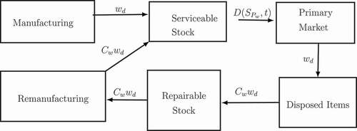
This model is developed to reduce the waste items and GHGs with CEs penalty tax ($Jaberet.al2013$) (Jaber, Glock, and El Saadany 2013). On the other side, the involvement of capacity constraints (CC) taken over by the conditions of owned and rented warehouse w.r.t. the lot-sizes of production and rework. Concisely, the system cost parameters considered in the model are listed below, and the following figure illustrates the process of serviceable and repairable stocks.

Figure 1. Manufacturing and Remanufacturing process for the waste items

5.1. Cost functions

The annual expected holding cost (AEHC) for the serviceable stock is

$A{H}_{ss}^w=\frac{h_{mss}\left(\frac{n{Q}_{mls}^2}{2D(S_{P_w},t)}-\frac{n^2{Q}_{mls}^2}{2{\delta }_{mr}}+\frac{Q_{mls}^{2}n(n-1)}{2{\delta }_{mr}}\right)+h_{rss}\left(\frac{m{R}_{rls}^2}{2C_w^{2}D(S_{P_w},t)}-\frac{m^2{R}_{rls}^2}{2{\delta }_{rr}{C}_w^2}+\frac{R_{rls}^{2}m(m-1)}{2{\delta }_{rr}{C}_w^2}\right)}{{\mu }_t}$

By using the Eqs.(1)(1) $\mathrm{T}\mathrm{h}\mathrm{a}\mathrm{t}\mathrm{i}\mathrm{s},{\mu }_t=\frac{n{Q}_{mls}(w_d+{\eta }_2)}{w_{d}D(S_{P_w},t)}$(1) , (2(2) $R_{rls}=C_w\lambda$(2) ) and Appendix I,

$A{H}_{ss}^w=\frac{Q_{mls}D(S_{P_w},t)}{2(w_d+{\eta }_2)}\left\{h_{mss}\left(\frac{1}{D(S_{P_w},t)}-\frac{1}{{\delta }_{mr}}\right)+\frac{h_{rss}{\eta }_{2}n}{2w_{d}m}\left(\frac{1}{D(S_{P_w},t)}-\frac{1}{{\delta }_{rr}}\right)\right\}$

The AEHC for the repairable stock is,

$A{H}_{rs}^w=\frac{h_{rrs}\left\{\frac{m{R}_{rls}^2}{2{\delta }_{rr}{C}_w^2}+\frac{m(m-1)R_{rls}^2}{C_w^{2}D(S_{P_w},t)}+\frac{{\mu }_t}{2}-\frac{n{\eta }_1{Q}_{mls}}{C_w(1-{\eta }_1)}(\frac{(m-1)R_{rls}}{D(S_{P_w},t)}+\frac{R_{rls}}{{\delta }_{rr}})\right\}}{{\mu }_t}$

Similarly, using the Eqs.(1)(1) $\mathrm{T}\mathrm{h}\mathrm{a}\mathrm{t}\mathrm{i}\mathrm{s},{\mu }_t=\frac{n{Q}_{mls}(w_d+{\eta }_2)}{w_{d}D(S_{P_w},t)}$(1) , (2(2) $R_{rls}=C_w\lambda$(2) ) and simplifying we get,

$A{H}_{rs}^w=\frac{h_{rrs}{w}_{d}D(S_{P_w},t)}{(w_d+{\eta }_2)}\left\{\frac{n{Q}_{mls}{\eta }_2^2}{2w_d^{2}m}\left(\frac{1}{2{\delta }_{rr}}-\frac{(m-1)}{2D(S_{P_w},t)}\right)+\frac{{\eta }_1(w_d+{\eta }_1)}{2w_{d}D(S_{P_w},t)}\right.$

$\left.-\frac{{\eta }_1{\eta }_{2}n{Q}_{mls}}{(1-{\eta }_1)w_{d}m}\left(\frac{(m-1)}{D(S_{P_w},t)}+\frac{1}{{\delta }_{rr}}\right)\right\}$

The annual production setup cost is the sum of the setup costs for all manufacturing and remanufacturing runs per cycle divided by the cycle time ${\mu }_t$.

The expected setup cost is,

$A{S}_c^w=\frac{(n{S}_c^m+m{S}_c^r)}{{\mu }_t}$

From the Eqs.(1)(1) $\mathrm{T}\mathrm{h}\mathrm{a}\mathrm{t}\mathrm{i}\mathrm{s},{\mu }_t=\frac{n{Q}_{mls}(w_d+{\eta }_2)}{w_{d}D(S_{P_w},t)}$(1) , (2(2) $R_{rls}=C_w\lambda$(2) ) we get,

$\mathrm{T}\mathrm{h}\mathrm{a}\mathrm{t}\mathrm{i}\mathrm{s},A{S}_c^w=\frac{w_{d}D(S_{P_w},t)(n{S}_c^m+m{S}_c^r)}{n{Q}_{mls}(w_d+{\eta }_2)}$

The annual production cost is the variable production cost per unit for all manufactured and remanufactured items per cycle divided by the cycle time $({\mu }_t)$ is,

$A{P}_c^w=\frac{n{Q}_{mls}{M}_c^w+m{R}_{rls}{R}_c^w}{{\mu }_t}$

$\mathrm{I}\mathrm{t}\mathrm{c}\mathrm{a}\mathrm{n}\mathrm{b}\mathrm{e}\mathrm{w}\mathrm{r}\mathrm{i}\mathrm{t}\mathrm{t}\mathrm{e}\mathrm{n}\mathrm{a}\mathrm{s},A{P}_c^w=\frac{D(S_{P_w},t)(M_c^w{w}_d+{\eta }_2{R}_c^w)}{(w_d+{\eta }_1)}$

According to Jaber et.al (Jaber, Glock, and El Saadany 2013) the annual cost of waste disposal is,

$A{W}_d^c=C_{w}D(S_{P_w},t)(1-{\eta }_1)$

From Bozorgi et.al (2014), the annual transportation cost is (fixed),

$A{C}_t^w=\frac{(n{Q}_{mls}+m{R}_{rls})C_F^w}{t_c^w{\mu }_t}+\frac{{\eta }_1{C}_F^w}{t_c^w}=\frac{C_F^w}{t_c^w}\left(D(S_{P_w},t)+{\eta }_2\right)$

In 2013, Jaber et al. defined the cost of GHGs for manufacturing and remanufacturing as,

$A{C}_{GH{G}_e}^w=D(S_{P_w},t)\left((m_1{\delta }_{mr}^2-m_2{\delta }_{mr}+m_3)(1-{\eta }_2)+(r_1{\delta }_{rr}^2-r_2{\delta }_{rr}+r_3)({\eta }_2)\right)$

by assumptions in (Section 6.2),

$A{C}_{GH{G}_e}^w=D(S_{P_w},t)\left((1-{\eta }_2)GH{G}_{EM}+{\eta }_{2}GH{G}_{ER}\right)$

In Jaber et al. (Jaber, Bazan, and El Saadany 2015) the annual cost of GHGs from transportation is,

$A{C}_{GH{G}_t}^w=\left(\frac{D(S_{P_w},t)}{t_c^w}+\frac{D(S_{P_w},t){\eta }_2}{t_c^w}\right)(GH{G}_{cet}GH{G}_{gt}GH{G}_{et})$

$A{C}_{GH{G}_t}^w=\frac{D(S_{P_w},t)(GH{G}_{cet}GH{G}_{gt}GH{G}_{et}){\eta }_2}{t_c^w}$

In Section 6.2, we define an annual penalty system cost of GHGs for production and rework. An emissions penalty scheme that penalizes the system for exceeding various permissible emission levels are given as,

$A{C}_{GH{G}_{pc}}^w={\mathrm{\Phi }}_M{E}_{p{c}_i}+{\mathrm{\Phi }}_R{E}_{p{c}_j}$

Li and Kara (2011) presented a relationship between the energy used by a machine tool for processing and the number of units processed.

The annual cost of energy used per year for manufacturing and remanufacturing is,

$A{E}_c^w=\frac{E_c^w\left\{\left({c{ }^{\mathrm{\prime }}}_m+\frac{{c{ }^{\mathrm{\prime }\mathrm{\prime }}}_m}{{\delta }_{mr}}\right)n{Q}_{mls}+\left({C{ }^{\mathrm{\prime }}}_r+\frac{{C{ }^{\mathrm{\prime }\mathrm{\prime }}}_r}{{\delta }_{rr}}\right)m{R}_{rls}\right\}}{{\mu }_t}$

$A{E}_c^w=\frac{E_c^w{w}_{d}D(S_{P_w},t)}{(w_d+{\eta }_2)}\left\{\left({c{ }^{\mathrm{\prime }}}_m+\frac{{c{ }^{\mathrm{\prime }\mathrm{\prime }}}_m}{{\delta }_{mr}}\right)+\left({C{ }^{\mathrm{\prime }}}_r+\frac{{C{ }^{\mathrm{\prime }\mathrm{\prime }}}_r}{{\delta }_{rr}}\right)\left(\frac{{\eta }_2}{w_d}\right)\right\}$

In this model, the contribution of promotional effort is most important to maximize the profit. Under a remanufacturing batch size, the promotional effort cost is solved in Section 6.3 and Appendix II,

$PE{C}^w=K(\rho -1{)}^2{\left\{\left(\frac{{\theta }_1-{\theta }_2{S}_{P_w}}{{\theta }_4}\right)(e^{{\theta }_4\pi }-1)\right\}}^{{\theta }_5}$

The annual purchasing and selling cost is given by

$A{C}_{ps}^w={\eta }_{2}D(S_{P_w},t)[P_C^w+S_P^w]$

5.2. Annual total expected cost function (ATECF)

The environmentally associated costs are concerned with GHGs from manufacturing, remanufacturing and transporting products. The value of $ATE{C}^w$ is calculated by using above cost functions.

$ATE{C}^w=A{H}_{ss}^w+A{H}_{rs}^w+A{S}_c^w+A{P}_c^w+A{W}_d^w+A{C}_t^w+A{C}_{GH{G}_e}^w+A{C}_{GH{G}_t}^w$

(8) $+A{C}_{GH{G}_{pc}}^w+A{E}_c^w+A{C}_{ps}^w+PE{C}^w$(8)

$ATE{C}^w=\frac{Q_{mls}D(S_{P_w},t)}{2(w_d+{\eta }_2)}\left\{h_{mss}{w}_d\left(\frac{1}{D(S_{P_w},t)}-\frac{1}{{\delta }_{mr}}\right)\right.$

(9) $+\left.\frac{h_{rss}{\eta }_{2}n}{2w_{d}m}\left(\frac{1}{D(S_{P_w},t)}-\frac{1}{{\delta }_{rr}}\right)\right\}+\mathrm{\Delta }$(9)

$\mathrm{w}\mathrm{h}\mathrm{e}\mathrm{r}\mathrm{e},\mathrm{\Delta }=\frac{h_{rrs}{w}_{d}D(S_{P_w},t)}{(w_d+{\eta }_2)}\left\{\frac{n{Q}_{mls}{\eta }_2^2}{2w_d^{2}m}\left(\frac{1}{2{\delta }_{rr}}-\frac{(m-1)}{2D(S_{P_w},t)}\right)+\frac{{\eta }_1(w_d+{\eta }_1)}{2w_{d}D(S_{P_w},t)}\right.$

$\left.-\frac{{\eta }_1{\eta }_{2}n{Q}_{mls}}{(1-{\eta }_1)w_{d}m}\left(\frac{(m-1)}{D(S_{P_w},t)}+\frac{1}{{\delta }_{rr}}\right)\right\}+\frac{w_{d}D(S_{P_w},t)(n{S}_c^m+m{S}_c^r)}{n{Q}_{mls}(w_d+{\eta }_2)}$

$+\frac{D(S_{P_w},t)(M_c^w{w}_d+{\eta }_2{R}_c^w)}{(w_d+{\eta }_1)}+C_{w}D(S_{P_w},t)(1-{\eta }_1)$

$+D(S_{P_w},t)\left((1-{\eta }_2)GH{G}_{EM}+{\eta }_{2}GH{G}_{ER}\right)\left({\mathrm{\Phi }}_M{E}_{p{c}_i}+{\mathrm{\Phi }}_R{E}_{p{c}_j}\right)$

$+\frac{D(S_{P_w},t)(GH{G}_{cet}GH{G}_{gt}GH{G}_{et}){\eta }_2}{t_c^w}+\frac{C_F^w}{t_c^w}\left(D(S_{P_w},t)+{\eta }_2\right)$

$+\frac{E_c^w{w}_{d}D(S_{P_w},t)}{(w_d+{\eta }_2)}\left\{\left({c{ }^{\mathrm{\prime }}}_m+\frac{{c{ }^{\mathrm{\prime }\mathrm{\prime }}}_m}{{\delta }_{mr}}\right)+\left({C{ }^{\mathrm{\prime }}}_r+\frac{{C{ }^{\mathrm{\prime }\mathrm{\prime }}}_r}{{\delta }_{rr}}\right)\left(\frac{{\eta }_2}{w_d}\right)\right\}$

$+K(\rho -1{)}^2{\left\{\left(\frac{{\theta }_1-{\theta }_2{S}_{P_w}}{{\theta }_4}\right)(e^{{\theta }_4\pi }-1)\right\}}^{{\theta }_5}+{\eta }_{2}D(S_{P_w},t)[P_C^w+S_P^w]$

Now, we have a solution procedure to find the optimal solution and minimum cost of the Eqn.(9)(9) $+\left.\frac{h_{rss}{\eta }_{2}n}{2w_{d}m}\left(\frac{1}{D(S_{P_w},t)}-\frac{1}{{\delta }_{rr}}\right)\right\}+\mathrm{\Delta }$(9) w.r.t. the decision variables. The following solution procedure gives the convexity of the Eqn.(9)(9) $+\left.\frac{h_{rss}{\eta }_{2}n}{2w_{d}m}\left(\frac{1}{D(S_{P_w},t)}-\frac{1}{{\delta }_{rr}}\right)\right\}+\mathrm{\Delta }$(9) .

5.2.1. Solution procedure

Differentiating partially w.r.t. $n$ by (9) we get,

(10) $\frac{\mathrm{\partial }ATE{C}^w(n,m,Q_{mls},R_{rls})}{\mathrm{\partial }n}=\frac{Q_{mls}D(S_{P_w},t)}{2{\delta }_{mr}(w_d+{\eta }_2)}\left(\frac{h_{rss}{\eta }_2}{2w_{d}m}\left(\frac{1}{D(S_{P_w},t)}-\frac{1}{{\delta }_{rr}}\right)\right)+{\mathrm{\Gamma }}_1$(10)

$\mathrm{w}\mathrm{h}\mathrm{e}\mathrm{r}\mathrm{e},{\mathrm{\Gamma }}_1=\frac{h_{rrs}{w}_{d}D(S_{P_w},t)}{(w_d+{\eta }_2)}\left\{\frac{Q_{mls}{\eta }_2^2}{2w_d^{2}m}\left(\frac{1}{2{\delta }_{rr}}-\frac{(m-1)}{2D(S_{P_w},t)}\right)\right.$

$\left.-\frac{{\eta }_1{\eta }_2{Q}_{mls}}{(1-{\eta }_1)w_{d}m}\left(\frac{(m-1)}{D(S_{P_w},t)}+\frac{1}{{\delta }_{rr}}\right)\right\}$

$-\frac{m{w}_{d}D(S_{P_w},t)S_c^m}{n^2{Q}_{mls}(w_d+{\eta }_2)}-\frac{{\theta }_3{(\rho -1)}^2}{n^{2}m}{\left\{\left(\frac{{\theta }_1-{\theta }_2{S}_{P_w}}{{\theta }_4}\right)(e^{{\theta }_4\pi }-1)\right\}}^{{\theta }_5}$

Differentiating again w.r.t. $n$ by (10) we get,

(11) $\frac{{\mathrm{\partial }}^{2}ATE{C}^w(n,m,Q_{mls},R_{rls})}{\mathrm{\partial }{n}^2}=\frac{m{w}_{d}D(S_{P_w},t)S_c^m}{n^3{Q}_{mls}(w_d+{\eta }_2)}+{\mathrm{\Gamma }}_2>0$(11)

$\mathrm{w}\mathrm{h}\mathrm{e}\mathrm{r}\mathrm{e},{\mathrm{\Gamma }}_2=\frac{{\theta }_3{(\rho -1)}^2}{n^{3}m}{\left\{\left(\frac{{\theta }_1-{\theta }_2{S}_{P_w}}{{\theta }_4}\right)(e^{{\theta }_4\pi }-1)\right\}}^{{\theta }_5}$

Differentiating partially w.r.t. $m$ by (9) we get,

(12) $\frac{\mathrm{\partial }ATE{C}^w(n,m,Q_{mls},R_{rls})}{\mathrm{\partial }m}=\frac{-Q_{mls}D(S_{P_w,t})h_{rss}{\eta }_2}{4m^2{w}_d{\delta }_{rr}(w_d+{\eta }_2)}\left(\frac{1}{D(S_{P_w},t)}-\frac{1}{{\delta }_{rr}}\right)+{\mathrm{\Gamma }}_3$(12)

$\mathrm{w}\mathrm{h}\mathrm{e}\mathrm{r}\mathrm{e},{\mathrm{\Gamma }}_3=\frac{h_{rrs}{w}_{d}D(S_{P_w},t)}{(w_d+{\eta }_2)}\left\{\frac{-n{Q}_{mls}{\eta }_2^2}{4w_d^2{m}^2{\delta }_{rr}}-\frac{n{Q}_{mls}{\eta }_2^2}{4w_d^2{m}^{2}D(S_{P_w,t})}\right.$

$\left.-\frac{n{\eta }_1{\eta }_2{Q}_{mls}D(S_{P_w},t)}{+}\frac{n{\eta }_1{\eta }_2{Q}_{mls}}{(1-{\eta }_1)w_d{\delta }_{rr}{m}^2}\right\}-\frac{w_{d}D(S_{P_w},t)S_c^r}{n{Q}_{mls}(w_d+{\eta }_2)}$

$+\frac{{\theta }_3{(\rho -1)}^2}{n{m}^2}{\left\{\left(\frac{{\theta }_1-{\theta }_2{S}_{P_w}}{{\theta }_4}\right)(e^{{\theta }_4\pi }-1)\right\}}^{{\theta }_5}$

Differentiating again w.r.t. $m$ by (12) we get,

(13) $\frac{{\mathrm{\partial }}^{2}ATE{C}^w(n,m,Q_{mls},R_{rls})}{\mathrm{\partial }{m}^2}=\frac{Q_{mls}D(S_{P_w,t})h_{rss}{\eta }_2}{2m^3{w}_d{\delta }_{rr}(w_d+{\eta }_2)}\left(\frac{1}{D(S_{P_w},t)}-\frac{1}{{\delta }_{rr}}\right)+{\mathrm{\Gamma }}_4>0$(13)

$\mathrm{w}\mathrm{h}\mathrm{e}\mathrm{r}\mathrm{e},{\mathrm{\Gamma }}_4=\frac{h_{rrs}{w}_{d}D(S_{P_w},t)}{(w_d+{\eta }_2)}\left\{\frac{n{Q}_{mls}{\eta }_2^2}{2w_d^2{m}^3}\left(\frac{1}{{\delta }_{rr}}+\frac{1}{D(S_{P_w},t)}\right)\right.$

$+\left.\frac{2n{\eta }_1{\eta }_2{Q}_{mls}}{m^3(1-{\eta }_1)w_{d}D(S_{P_w},t)}\left(\frac{1}{D(S_{P_w},t)}-\frac{1}{{\delta }_{rr}}\right)\right\}$

$+\frac{2{\theta }_3{(\rho -1)}^2}{n{m}^3}{\left\{\left(\frac{{\theta }_1-{\theta }_2{S}_{P_w}}{{\theta }_4}\right)(e^{{\theta }_4\pi }-1)\right\}}^{{\theta }_5}$

Differentiating partially w.r.t. $Q_{mls}$ by (9) we get,

$\frac{\mathrm{\partial }ATE{C}^w(n,m,Q_{mls},R_{rls})}{\mathrm{\partial }{Q}_{mls}}=\frac{D(S_{P_w},t)}{2(w_d+{\eta }_2)}\left\{h_{mss}{w}_d\left(\frac{1}{D(S_{P_w},t)}-\frac{1}{{\delta }_{mr}}\right)\right.$

$+\left.\frac{h_{rss}n{\eta }_2}{2w_{d}m}\left(\frac{1}{D(S_{P_w},t)}-\frac{1}{{\delta }_{rr}}\right)\right\}$

$+\frac{h_{rrs}{w}_{d}D(S_{P_w},t)}{(w_d+{\eta }_2)}\left\{\frac{n{\eta }_2^2}{2w_d^{2}m}\left(\frac{1}{2{\delta }_{rr}}-\frac{(m-1)}{2D(S_{P_w},t)}\right)\right.$

$-\left.\frac{n{\eta }_1{\eta }_2}{(1-{\eta }_1)w_{d}m}\left(\frac{(m-1)}{D(S_{P_w},t)}+\frac{1}{{\delta }_{rr}}\right)\right\}$

(14) $-\frac{w_{d}D(S_{P_w},t)(n{S}_c^m+m{S}_c^r)}{n{Q}_{mls}^2(w_d+{\eta }_2)}$(14)

Differentiating again w.r.t.. $Q_{mls}$ by (14) we get,

(15) $\frac{{\mathrm{\partial }}^{2}ATE{C}^w(n,m,Q_{mls},R_{rls})}{\mathrm{\partial }{Q}_{mls}^2}=\frac{2w_{d}D(S_{P_w},t)(n{S}_c^m+m{S}_c^r)}{n{Q}_{mls}^3(w_d+{\eta }_2)}>0$(15)

From the Eqs.(11)(11) $\frac{{\mathrm{\partial }}^{2}ATE{C}^w(n,m,Q_{mls},R_{rls})}{\mathrm{\partial }{n}^2}=\frac{m{w}_{d}D(S_{P_w},t)S_c^m}{n^3{Q}_{mls}(w_d+{\eta }_2)}+{\mathrm{\Gamma }}_2>0$(11) , (13(13) $\frac{{\mathrm{\partial }}^{2}ATE{C}^w(n,m,Q_{mls},R_{rls})}{\mathrm{\partial }{m}^2}=\frac{Q_{mls}D(S_{P_w,t})h_{rss}{\eta }_2}{2m^3{w}_d{\delta }_{rr}(w_d+{\eta }_2)}\left(\frac{1}{D(S_{P_w},t)}-\frac{1}{{\delta }_{rr}}\right)+{\mathrm{\Gamma }}_4>0$(13) ), and (15(15) $\frac{{\mathrm{\partial }}^{2}ATE{C}^w(n,m,Q_{mls},R_{rls})}{\mathrm{\partial }{Q}_{mls}^2}=\frac{2w_{d}D(S_{P_w},t)(n{S}_c^m+m{S}_c^r)}{n{Q}_{mls}^3(w_d+{\eta }_2)}>0$(15) ) the second derivative of the decision variables $n,m,Q_{mls}$ are greater than zero. Thus, the total cost function (9) $ATE{C}^w$ is convex and it attains a minimum cost w.r.t. the decision variables.

From, (14) and (2) we obtain the optimal solutions for manufacturing and remanufacturing lot-sizes.

The manufacturing lot-size $Q_{mls}$ is written as follows,

(16) $Q_{mls}=\sqrt{\frac{w_{d}D(S_{P_w},t)\left(n{S}_c^m+m{S}_c^r\right)}{n(w_d+{\eta }_2)z_1}}$(16)

$\mathrm{w}\mathrm{h}\mathrm{e}\mathrm{r}\mathrm{e},z_1=\frac{D(S_{P_w},t)}{2(w_d+{\eta }_2)}\left\{h_{mss}{w}_d\left(\frac{1}{D(S_{P_w},t)}-\frac{1}{{\delta }_{mr}}\right)\right.$

$+\left.\frac{h_{rss}n{\eta }_2}{2w_{d}m}\left(\frac{1}{D(S_{P_w},t)}-\frac{1}{{\delta }_{rr}}\right)\right\}$

$+\frac{h_{rrs}{w}_{d}D(S_{P_w},t)}{(w_d+{\eta }_2)}\left\{\frac{n{\eta }_2^2}{2w_d^{2}m}\left(\frac{1}{2{\delta }_{rr}}-\frac{(m-1)}{2D(S_{P_w},t)}\right)\right.$

$-\left.\frac{n{\eta }_1{\eta }_2}{(1-{\eta }_1)w_{d}m}\left(\frac{(m-1)}{D(S_{P_w},t)}+\frac{1}{{\delta }_{rr}}\right)\right\}$

The remanufacturing lot-size $R_{rls}$ is written as follows,

(17) $R_{rls}=\frac{C_w{\eta }_{2}n{Q}_{mls}}{w_{d}m}$(17)

5.3. ATECF with capacity constraint (CC)

In this section, we disscuss the impact of warehouse constraints for the annual holding cost. Here, we have two types of holding costs for the manufacturing and remanufacturing items under serviceable stocks. The optimal solutions of manufacturing and remanufacturing lot-sizes of the total cost function (9) can be classified by two models for the CC.

In Model I and Model II, if the optimal solutions of (9) (w.r.t. given numerical parameters) is $R_{rls}>C_{ow}$ and $Q_{mls}<C_{ow}$ then, by the assumptions of Section 6.4, we calculate manufacturing holding cost only for OW and remanufacturing holding cost only for RW.

Model I

In this model, the manufacturing lot-size is less than or equal to the capacity of the OW (i.e. $Q_{mls}\le C_{ow}$) by using Section 6.4 and Appendix III, we find the annual holding cost for manufacturing for a owned warehouse (OW) as follows,

(18) $A{H}_{ow}^w=\frac{h_{mss}({\theta }_1-{\theta }_2{S}_{P_w})}{n\pi ({\theta }_4+{\alpha }_{ow})}\left\{\frac{1}{{\alpha }_{ow}}-\frac{e^{{\theta }_4\pi }}{{\theta }_4}+\frac{1}{{\theta }_4}\right\}$(18)

Now, we characterized the total cost function ($ATE{C}_{ow}^w$) in owned warehouse (OW) is

(19) $ATE{C}_{ow}^w=\frac{h_{mss}({\theta }_1-{\theta }_2{S}_{P_w})}{n\pi ({\theta }_4+{\alpha }_{ow})}\left\{\frac{1}{{\alpha }_{ow}}-\frac{e^{{\theta }_4\pi }}{{\theta }_4}+\frac{1}{{\theta }_4}\right\}+\mathrm{\Delta }$(19)

Now, we have a solution procedure to find the optimal solution and minimum cost of the Eqn.(19(19) $ATE{C}_{ow}^w=\frac{h_{mss}({\theta }_1-{\theta }_2{S}_{P_w})}{n\pi ({\theta }_4+{\alpha }_{ow})}\left\{\frac{1}{{\alpha }_{ow}}-\frac{e^{{\theta }_4\pi }}{{\theta }_4}+\frac{1}{{\theta }_4}\right\}+\mathrm{\Delta }$(19) ) $(ATE{C}_{ow}^w)$ w.r.t. the decision variables of production and rework.

5.3.1 Solution procedure

Differentiating partially w.r.t. $n$ by (19),

(20) $\frac{\mathrm{\partial }ATE{C}_{ow}^w(n,m,Q_{mls},R_{rls})}{\mathrm{\partial }n}=\frac{-h_{mss}({\theta }_1-{\theta }_2{S}_{P_w})}{n^2\pi ({\theta }_4+{\alpha }_{ow})}\left\{\frac{1}{{\alpha }_{ow}}-\frac{e^{{\theta }_4\pi }}{{\theta }_4}+\frac{1}{{\theta }_4}\right\}+{\mathrm{\Gamma }}_1$(20)

Differentiating again w.r.t. $n$ by (20),

(21) $\frac{{\mathrm{\partial }}^{2}ATE{C}_{ow}^w(n,m,Q_{mls},R_{rls})}{\mathrm{\partial }{n}^2}=\frac{-h_{mss}({\theta }_1-{\theta }_2{S}_{P_w})}{n^2\pi ({\theta }_4+{\alpha }_{ow})}\left\{\frac{1}{{\alpha }_{ow}}-\frac{e^{{\theta }_4\pi }}{{\theta }_4}+\frac{1}{{\theta }_4}\right\}+{\mathrm{\Gamma }}_2>0$(21)

If we differentiating partially w.r.t. $m$ by (19) then, we get (22) = (12)

(i.e.)

(22) $\frac{\mathrm{\partial }ATE{C}_{ow}^w(n,m,Q_{mls},R_{rls})}{\mathrm{\partial }m}=\frac{\mathrm{\partial }ATE{C}^w(n,m,Q_{mls},R_{rls})}{\mathrm{\partial }m}$(22)

Similarly, if we differentiating again w.r.t. $m$ by (22) then, we get (23) = (13)

(i.e.)

(23) $\frac{{\mathrm{\partial }}^{2}ATE{C}_{ow}^w(n,m,Q_{mls},R_{rls})}{\mathrm{\partial }{m}^2}=\frac{{\mathrm{\partial }}^{2}ATE{C}^w(n,m,Q_{mls},R_{rls})}{\mathrm{\partial }{m}^2}>0.$(23)

Differentiating partially w.r.t. $Q_{mls}$ by (19)

$\frac{\mathrm{\partial }ATE{C}_{ow}^w(n,m,Q_{mls},R_{rls})}{\mathrm{\partial }{Q}_{mls}}=\frac{h_{rrs}{w}_{d}D(S_{P_w},t)}{(w_d+{\eta }_2)}\left\{\frac{n{\eta }_2^2}{2w_d^{2}m}\left(\frac{1}{2{\delta }_{rr}}-\frac{(m-1)}{2D(S_{P_w},t)}\right)\right.$

$-\left.\frac{n{\eta }_1{\eta }_2}{(1-{\eta }_1)w_{d}m}\left(\frac{(m-1)}{D(S_{P_w},t)}+\frac{1}{{\delta }_{rr}}\right)\right\}$

(24) $-\frac{w_{d}D(S_{P_w},t)(n{S}_c^m+m{S}_c^r)}{n{Q}_{mls}^2(w_d+{\eta }_2)}$(24)

Differentiating again w.r.t. $Q_{mls}$ by (24)

(25) $\frac{{\mathrm{\partial }}^{2}ATE{C}_{ow}^w(n,m,Q_{mls},R_{rls})}{\mathrm{\partial }{Q}_{mls}^2}=\frac{2w_{d}D(S_{P_w},t)(n{S}_c^m+m{S}_c^r)}{n{Q}_{mls}^3(w_d+{\eta }_2)}>0.$(25)

From the Eqs.(21)(21) $\frac{{\mathrm{\partial }}^{2}ATE{C}_{ow}^w(n,m,Q_{mls},R_{rls})}{\mathrm{\partial }{n}^2}=\frac{-h_{mss}({\theta }_1-{\theta }_2{S}_{P_w})}{n^2\pi ({\theta }_4+{\alpha }_{ow})}\left\{\frac{1}{{\alpha }_{ow}}-\frac{e^{{\theta }_4\pi }}{{\theta }_4}+\frac{1}{{\theta }_4}\right\}+{\mathrm{\Gamma }}_2>0$(21) , (23(23) $\frac{{\mathrm{\partial }}^{2}ATE{C}_{ow}^w(n,m,Q_{mls},R_{rls})}{\mathrm{\partial }{m}^2}=\frac{{\mathrm{\partial }}^{2}ATE{C}^w(n,m,Q_{mls},R_{rls})}{\mathrm{\partial }{m}^2}>0.$(23) ), and (25(25) $\frac{{\mathrm{\partial }}^{2}ATE{C}_{ow}^w(n,m,Q_{mls},R_{rls})}{\mathrm{\partial }{Q}_{mls}^2}=\frac{2w_{d}D(S_{P_w},t)(n{S}_c^m+m{S}_c^r)}{n{Q}_{mls}^3(w_d+{\eta }_2)}>0.$(25) ) the second derivative of the decision variables $n,m,Q_{mls}$ is greater than zero. Thus, the total cost function (19) is convex, and it attains a minimum cost w.r.t. the decision variables.

From Eqn.(24)(24) $-\frac{w_{d}D(S_{P_w},t)(n{S}_c^m+m{S}_c^r)}{n{Q}_{mls}^2(w_d+{\eta }_2)}$(24) , we obtain the manufacturing lot-size $Q_{mls}$,

(26) $Q_{mls}=\sqrt{\frac{w_{d}D(S_{P_w},t)(n{S}_c^m+m{S}_c^r)}{n(w_d+{\eta }_2)z_2}}$(26)

$\mathrm{w}\mathrm{h}\mathrm{e}\mathrm{r}\mathrm{e},z_2=\frac{h_{rrs}{w}_{d}D(S_{P_w},t)}{(w_d+{\eta }_2)}\left\{\frac{n{\eta }_2^2}{2w_d^{2}m}\left(\frac{1}{2{\delta }_{rr}}-\frac{(m-1)}{2D(S_{P_w},t)}\right)\right.$

$-\left.\frac{n{\eta }_1{\eta }_2}{(1-{\eta }_1)w_{d}m}\left(\frac{(m-1)}{D(S_{P_w},t)}+\frac{1}{{\delta }_{rr}}\right)\right\}$

From Eqn.(2)(2) $R_{rls}=C_w\lambda$(2) we obtain the remanufacturing lot-size $R_{rls}$,

Model II

In this model, the remanufacturing lot-size is greater than the capacity of the OW.

(i.e. $R_{mls}>C_{ow}$) by using Section 6.4 and Appendix III.

Then, the annual holding cost for remanufacturing in rented warehouse (RW) is

(27) $A{H}_{rw}^w=\frac{h_{rss}({\theta }_1-{\theta }_2{S}_{P_w})}{wm\pi ({\theta }_4+{\alpha }_{rw})}\left\{\frac{1}{{\alpha }_{rw}}-\frac{e^{{\theta }_4\pi }}{{\theta }_4}+\frac{1}{{\theta }_4}\right\}$(27)

Now, we characterized the total cost function ($ATE{C}_{rw}^w$) in OW is

(28) $ATE{C}_{rw}^w=\frac{h_{rss}({\theta }_1-{\theta }_2{S}_{P_w})}{wm\pi ({\theta }_4+{\alpha }_{rw})}\left\{\frac{1}{{\alpha }_{rw}}-\frac{e^{{\theta }_4\pi }}{{\theta }_4}+\frac{1}{{\theta }_4}\right\}+\mathrm{\Delta }$(28)

where, the value of $\mathrm{\Delta }$ is in (9).

5.3.2 Solution procedure

By differentiating (28) w.r.t. $n$, we get the values of the Eqn.(20)(20) $\frac{\mathrm{\partial }ATE{C}_{ow}^w(n,m,Q_{mls},R_{rls})}{\mathrm{\partial }n}=\frac{-h_{mss}({\theta }_1-{\theta }_2{S}_{P_w})}{n^2\pi ({\theta }_4+{\alpha }_{ow})}\left\{\frac{1}{{\alpha }_{ow}}-\frac{e^{{\theta }_4\pi }}{{\theta }_4}+\frac{1}{{\theta }_4}\right\}+{\mathrm{\Gamma }}_1$(20) .

(i.e.)

(29) $\frac{\mathrm{\partial }ATE{C}_{rw}^w(n,m,Q_{mls},R_{rls})}{\mathrm{\partial }n}=\frac{\mathrm{\partial }ATE{C}^w(n,m,Q_{mls},R_{rls})}{\mathrm{\partial }n}$(29)

Similarly, for the second derivative of (29) is equal to (22)

(i.e.)

(30) $\frac{{\mathrm{\partial }}^{2}ATE{C}_{rw}^w(n,m,Q_{mls},R_{rls})}{\mathrm{\partial }{n}^2}=\frac{{\mathrm{\partial }}^{2}ATE{C}^w(n,m,Q_{mls},R_{rls})}{\mathrm{\partial }{n}^2}>0.$(30)

Differentiating partially w.r.t. $m$ by Eqn.(28(28) $ATE{C}_{rw}^w=\frac{h_{rss}({\theta }_1-{\theta }_2{S}_{P_w})}{wm\pi ({\theta }_4+{\alpha }_{rw})}\left\{\frac{1}{{\alpha }_{rw}}-\frac{e^{{\theta }_4\pi }}{{\theta }_4}+\frac{1}{{\theta }_4}\right\}+\mathrm{\Delta }$(28) ),

(31) $\frac{\mathrm{\partial }ATE{C}_{rw}^w(n,m,Q_{mls},R_{rls})}{\mathrm{\partial }m}=\frac{-h_{rss}({\theta }_1-{\theta }_2{S}_{P_w})}{w{m}^2\pi ({\theta }_4+{\alpha }_{rw})}\left\{\frac{1}{{\alpha }_{rw}}-\frac{e^{{\theta }_4\pi }}{{\theta }_4}+\frac{1}{{\theta }_4}\right\}+{\mathrm{\Gamma }}_3$(31)

Differentiating again w.r.t. $m$ by (31),

(32) $\frac{{\mathrm{\partial }}^{2}ATE{C}_{rw}^w(n,m,Q_{mls},R_{rls})}{\mathrm{\partial }{m}^2}=\frac{2h_{rss}({\theta }_1-{\theta }_2{S}_{P_w})}{w{m}^3\pi ({\theta }_4+{\alpha }_{rw})}\left\{\frac{1}{{\alpha }_{rw}}-\frac{e^{{\theta }_4\pi }}{{\theta }_4}+\frac{1}{{\theta }_4}\right\}+{\mathrm{\Gamma }}_4>0$(32)

Differentiating w.r.t. $Q_{mls}$ by (28) we obtain the Eqn.(26)(26) $Q_{mls}=\sqrt{\frac{w_{d}D(S_{P_w},t)(n{S}_c^m+m{S}_c^r)}{n(w_d+{\eta }_2)z_2}}$(26) then, we can easily find the value of manufacturing lot-size $Q_{mls}$ for the RW. For solving remanufacturing lot-size $R_{rls}$ we use the Eqn.(2)(2) $R_{rls}=C_w\lambda$(2) .

Algorithm 5.1

Step 1 Set n = 1, m = 1. for all, $n,m>0$

Step 2 Find $Q_{mls}$ and $R_{rls}$

Step 3 Continue this process, if there is no different occurs in the values of $Q_{mls}$ and $R_{rls}$ (w.r.t. the changes of $n,m$) then, ($Q_{mls}^{\star }$, $R_{rls}^{\star }$), ($Q_{mls}^{\star o}$, $R_{rls}^{\star o}$), ($Q_{mls}^{\star r}$, $R_{rls}^{\star r}$) are the optimal solutions of the given total cost functions (9), (19), (28).

6. Numerical examples

Example 6.1. Input parameters and emission constraints of this model is given inTables 1 to 5. Numerical solutions of $ATE{C}^w$, $ATE{C}_{ow}^w$, and $ATE{C}_{rw}^w$ are shown inTables 6, 7, 8 by using algorithm al1. Further, all the solutions are in dollars ($).

Table 1. Comparitive literature of this study

Authors	Model	Emission	Items	Demand	Constraints
Chen et.al (Chen and Su 2020)	CSM	…	…	…	…
Herwich et.al (Hertwich et al. 2019)	…	GHG Penalty	…	…	…
Heydari et.al (Rezagholifam et al. 2020)	…	…	…	Price & stock	Capacity
Jaber et.al (Jaber, Bazan, and El Saadany 2015)		GHG Penalty	…	…	…
Lee et.al(Lee, Wang, and Chen 2017)	CSM	…	…	Stock	…
Ndhaief et.al (Ndhaief et al. 2020)	…	…	Reowrked	…	…
Palanivel et.al (Palanivel and Uthayakumar 2017)	…	…	…	Promotional effort	…
Tang et.al (Tang et al. 2018)	…	GHG Penalty	…	…	…
Present model	CSM	GHG Penalty	Reowrked	Promotional effort	Capacity

$\dots$ denotes that the articles doesn’t contain such topics.

Table 2. Emission constraints structure for manufacturing where, (i = 1, 2, … k)

Emission limits	Penalty cost ($E_{p{c}_i}$)
$D(S_{P_w},t)GH{G}_{EM}\le E_{M_1}$	$E_{p{c}_1}=0$
$E_{M_1}\le D(S_{P_w},t)GH{G}_{EM}\le E_{M_2}$	$E_{p{c}_2}$
$E_{M_2}\le D(S_{P_w},t)GH{G}_{EM}\le E_{M_3}$	$E_{p{c}_3}$
$⋮$	$⋮$
$⋮$	$⋮$
$E_{M_k}\le D(S_{P_w},t)GH{G}_{EM}$	$E_{p{c}_k}$
where, $E_{p{c}_k}>E_{p{c}_{k-1}}>\cdots >E_{p{c}_2}>E_{p{c}_1}=0$

Table 3. Emission constraints structure for remanufacturing where, (j = 1, 2, … q)

Emission limits	Penalty cost ($E_{p{c}_j}$)
$D(S_{P_w},t)GH{G}_{ER}\le E_{R_1}$	$E_{p{c}_1}=0$
$E_{R_1}\le D(S_{P_w},t)GH{G}_{ER}\le E_{R_2}$	$E_{p{c}_2}$
$E_{R_2}\le D(S_{P_w},t)GH{G}_{ER}\le E_{R_3}$	$E_{p{c}_3}$
$⋮$	$⋮$
$⋮$	$⋮$
$E_{R_q}\le D(S_{P_w},t)GH{G}_{ER}$	$E_{p{c}_q}$
where, $E_{p{c}_q}>E_{p{c}_{q-1}}>\cdots >E_{p{c}_2}>E_{p{c}_1}=0$

Table 4. Numerical input parameters and its values

Parameters	values	units	Parameters	values	units
${\alpha }_{ow}$	0.5	$/unit	$C_{ow}$	200	constant $/unit
${\alpha }_{rw}$	0.6	$/unit	$h_{mss}$	200	units/year
${\eta }_1$	0.6	$/unit	$h_{rss}$	100	“
${\eta }_2$	0.99	$/unit	$h_{rrs}$	60	“
${\pi }_0$	0.07	inventory length	$S_c^m$	1500	$/setup
${\pi }_1$	0.06	“	$S_c^r$	750	“
${\theta }_1$	2000	constant$>0$, $/unit	$E_c^w$	0.093	$/KWh
${\theta }_2$	10	“	$M_c^w$	35,000	$/unit
${\theta }_3$	2	“	$R_c^w$	15,000	“
${\theta }_4$	1	“	$C_w$	1200	“
${\theta }_5$ and $\rho$	1 and 2	$\rho \ne 1>$0, $/unit	$C_F^w$	1000	$/truck
${\delta }_{mr}$	2000	units/year	$t_c^w$	200	units/trucks
${\delta }_{rr}$	1800	“	$C_m$	60	KWh/unit
${\omega }_{m1}$	0.000008	$ton.yea{r}^2/uni{t}^3$	$C_m\prime$	180,000	KWh/year
${\omega }_{m2}$	0.000006	$ton.year/uni{t}^2$	$C_r$	35	KWh/unit
${\omega }_{m3}$	1	$ton./unit$	$C_r\prime$	60,000	KWh/year
${\omega }_{r1}$	0.000004	$ton.yea{r}^2/uni{t}^3$	$GH{G}_{cet}$	15	$/ton
${\omega }_{r2}$	0.000002	$ton.year/uni{t}^2$	$GH{G}_{gt}$	350	gallons/truck
${\omega }_{r3}$	2	$ton./unit$	$GH{G}_{et}$	0.01	ton /gallons
$S_{P_w}$	100	constant $/unit	$w_d$	600	waste/year
$P_{C_w}$	75	constant $/unit	$\pi$	0.08	total length

Table 5. Emission constraints structure for manufacturing and remanufacturing

Emission limits	Penalty cost ($E_{p{c}_i}$)
Penalty Emission limits for manufacturing	where, i = 1, 2, … k
$D(S_{P_w},t)GH{G}_{EM}\le 20000$	$0$
$20000\le D(S_{P_w},t)GH{G}_{EM}\le 45000$	$2000$
$45000\le D(S_{P_w},t)GH{G}_{EM}\le 60000$	$3000$
$60000\le D(S_{P_w},t)GH{G}_{EM}$	$4000$
where, $E_{p{c}_4}>E_{p{c}_3}>E_{p{c}_2}>E_{p{c}_1}=0$
Emission limits	Penalty cost ($E_{p{c}_j}$)
Penalty Emission limits for remanufacturing	where, j = 1, 2, … q
$D(S_{P_w},t)GH{G}_{ER}\le 15000$	$0$
$15000\le D(S_{P_w},t)GH{G}_{ER}\le 30000$	$500$
$30000\le D(S_{P_w},t)GH{G}_{ER}\le 45000$	$1000$
$45000\le D(S_{P_w},t)GH{G}_{ER}$	$1500$
where, $E_{p{c}_4}>E_{p{c}_3}>E_{p{c}_2}>E_{p{c}_1}=0$

Table 6. Total costs without CC $ATE{C}^w$

$n$	$m$	$Q_{mls}^{\star o}$	$R_{rls}^{\star o}$	$A{C}_{GH{G}_e}^w$	$A{C}_{GH{G}_t}^w$	$ATE{C}^w$
1	1	121.27	218.29	272,990	255.93	507,430
2	2	121.32	218.38	272,990	255.93	507,290
3	3	121.37	218.47	272,990	255.93	507,270
4	5	131.74	189.70	272,990	255.93	507,200
5	6	129.84	194.77	272,990	255.93	507,170
6	7	128.57	198.36	272,990	255.93	507,160
7	8	127.66	201.06	272,990	255.93	507,160
8	9	126.98	203.17	272,990	255.93	507,160
9	10	126.46	204.86	272,990	255.93	507,160 ${ }^{†}$
10	11	126.05	206.26	272,990	255.93	507,170
11	12	125.72	207.44	272,990	255.93	507,170
12	13	125.45	208.44	272,990	255.93	507,170

Table 7. Total costs with CC in owned warehouse $ATE{C}_{ow}^w$

$n$	$m$	$Q_{mls}^{\star o}$	$R_{rls}^{\star o}$	$A{C}_{GH{G}_e}^w$	$A{C}_{GH{G}_t}^w$	$ATE{C}_{ow}^w$
1	23	2785.4	218.00	272,990	255.93	488,030
2	34	2076.8	219.90	272,990	255.93	485,760
3	44	1803.5	221.34	272,990	255.93	485,170
4	51	1571.0	221.79	272,990	255.93	484,980
5	56	1381.3	221.99	272,990	255.93	484,940 ${ }^{†}$
6	61	1255.6	222.31	272,990	255.93	484,970
7	68	1201.8	222.69	272,990	255.93	485,020
8	75	1161.3	222.99	272,990	255.93	485,090
9	79	1087.9	223.09	272,990	255.93	485,180
10	85	1054.0	223.21	272,990	255.93	485,270

Table 8. Total costs with CC in rented warehouse $ATE{C}_{rw}^w$

$n$	$m$	$Q_{mls}^{\star r}$	$R_{rls}^{\star r}$	$A{C}_{GH{G}_e}^w$	$A{C}_{GH{G}_t}^w$	$ATE{C}_{rw}^w$
1	25	3060.4	220.35	267,580	250.86	473,320 ${ }^{†}$
2	36	2214.9	221.49	267,580	250.86	473,670
3	41	1677.8	220.98	267,580	250.86	473,970
4	50	1542.3	222.09	267,580	250.86	474,200
5	57	1409.9	222.62	267,580	250.86	474,410

7. Sensitivity analysis

This section provides the numerical changes of the rates (${\delta }_{mr},{\delta }_{rr}$), costs ($M_c^w$, $R_c^w$), and setup costs ($S_c^m,S_c^r$) of manufacturing and remanufacturing respectively. We consider the numerical changes w.r.to. $15\mathrm{\%}$, $25\mathrm{\%}$, and $50\mathrm{\%}$ by adding and subtracting in (${\delta }_{mr},{\delta }_{rr}$), costs ($M_c^w$, $R_c^w$), setup costs ($S_c^m,S_c^r$). Moreover, the solutions of $ATE{C}^w$, $ATE{C}_{ow}^w$, and $ATE{C}_{rw}^w$ are listed in Tables 9, 10, 11, 12, 13, 14, 15, 16, 17.

Table 9. List of optimal solutions for $ATE{C}^w$ w.r.to. the parameter changes in $15\mathrm{\%}$

Parameters	Changes in	$n$	$m$	$Q_{mls}^{\star }$	$R_{rls}^{\star }$	$A{C}_{GH{G}_e}^w$	$A{C}_{GH{G}_t}^w$	$ATE{C}^w$
${\delta }_{mr},{\delta }_{rr}$	$-15$%	5	6	129.84	194.77	272,990	255.93	507,250${ }^{†}$
${\delta }_{mr},{\delta }_{rr}$	$+15$%	5	6	129.84	194.77	272,990	255.93	507,250${ }^{†}$
$M_c^w$, $R_c^w$	$-15$%	5	6	133.46	200.19	199,870	255.93	434,660${ }^{†}$
$M_c^w$, $R_c^w$	$+15$%	5	6	126.51	189.76	406,230	255.93	640,370${ }^{†}$
$S_c^m,S_c^r$	$-15$%	5	6	119.73	179.59	272,990	255.93	504,130${ }^{†}$
$S_c^m,S_c^r$	$+15$%	5	6	139.23	208.84	272,990	255.93	510,160${ }^{†}$

Table 10. List of optimal solutions for $ATE{C}_{ow}^w$ w.r.to the parameter changes in $15\mathrm{\%}$

Parameters	Changes in	$n$	$m$	$Q_{mls}^{\star }$	$R_{rls}^{\star }$	$A{C}_{GH{G}_e}^w$	$A{C}_{GH{G}_t}^w$	$ATE{C}_{ow}^w$
${\delta }_{mr},{\delta }_{rr}$	$-15$%	5	57	1406.7	222.12	272,990	255.93	484,940${ }^{†}$
${\delta }_{mr},{\delta }_{rr}$	$+15$%	5	56	1381.3	221.99	272,990	255.93	484,940${ }^{†}$
$M_c^w$, $R_c^w$	$-15$%	5	53	1420.7	241.26	199,870	255.93	412,270${ }^{†}$
$M_c^w$, $R_c^w$	$+15$%	5	57	1307.6	206.46	406,230	255.93	618,080${ }^{†}$
$S_c^m,S_c^r$	$-15$%	5	58	1321.0	204.99	272,990	255.93	483,630${ }^{†}$
$S_c^m,S_c^r$	$+15$%	5	56	1480.9	238.00	272,990	255.93	486,150${ }^{†}$

Table 11. List of optimal solutions for $ATE{C}_{rw}^w$w.r.to the parameter changes in $15\mathrm{\%}$

Parameters	Changes in	$n$	$m$	$Q_{mls}^{\star }$	$R_{rls}^{\star }$	$A{C}_{GH{G}_e}^w$	$A{C}_{GH{G}_t}^w$	$ATE{C}_{rw}^w$
${\delta }_{mr},{\delta }_{rr}$	$-15$%	1	25	3060.4	220.35	272,990	250.86	473,320${ }^{†}$
${\delta }_{mr},{\delta }_{rr}$	$+15$%	1	25	3060.4	220.35	272,990	250.86	473,320${ }^{†}$
$M_c^w$, $R_c^w$	$-15$%	1	25	3357.4	241.76	195,910	250.86	402,100${ }^{†}$
$M_c^w$, $R_c^w$	$+15$%	1	25	2830.6	203.80	398,190	250.86	731,020${ }^{†}$
$S_c^m,S_c^r$	$-15$%	1	25	2822.6	203.23	267,580	250.86	472,130${ }^{†}$
$S_c^m,S_c^r$	$+15$%	1	26	3429.1	237.40	267,580	250.86	474,420${ }^{†}$

Table 12. List of optimal solutions for $ATE{C}^w$ w.r.to the parameter changes in $25\mathrm{\%}$

Parameters	Changes in	$n$	$m$	$Q_{mls}^{\star }$	$R_{rls}^{\star }$	$A{C}_{GH{G}_e}^w$	$A{C}_{GH{G}_t}^w$	$ATE{C}^w$
${\delta }_{mr},{\delta }_{rr}$	$-25$%	5	6	129.84	194.77	272,990	255.93	507,250${ }^{†}$
${\delta }_{mr},{\delta }_{rr}$	$+25$%	5	6	129.84	194.77	272,990	255.93	507,250${ }^{†}$
$M_c^w$, $R_c^w$	$-25$%	6	7	129.51	199.82	199,870	255.93	434,230${ }^{†}$
$M_c^w$, $R_c^w$	$+25$%	5	6	128.93	193.39	406,230	255.93	640,430${ }^{†}$
$S_c^m,S_c^r$	$-25$%	5	6	127.22	190.83	272,990	255.93	506,440${ }^{†}$
$S_c^m,S_c^r$	$+25$%	5	6	132.41	198.62	272,990	255.93	508,050${ }^{†}$

Table 13. List of optimal solutions for $ATE{C}_{ow}^w$w.r.to the parameter changes in $25\mathrm{\%}$

Parameters	Changes in	$n$	$m$	$Q_{mls}^{\star }$	$R_{rls}^{\star }$	$A{C}_{GH{G}_e}^w$	$A{C}_{GH{G}_t}^w$	$ATE{C}_{ow}^w$
${\delta }_{mr},{\delta }_{rr}$	$-25$%	6	66	1361.7	222.82	272,990	255.93	484,960${ }^{†}$
${\delta }_{mr},{\delta }_{rr}$	$+25$%	5	64	1590.4	223.65	272,990	255.93	484,940${ }^{†}$
$M_c^w$, $R_c^w$	$-25$%	5	61	1543.8	227.77	199,870	255.93	411,900${ }^{†}$
$M_c^w$, $R_c^w$	$+25$%	5	59	1428.3	217.88	406,230	255.93	618,120${ }^{†}$
$S_c^m,S_c^r$	$-25$%	6	62	1250.8	217.88	272,990	255.93	484,620$†$
$S_c^m,S_c^r$	$+25$%	5	57	1434.6	226.52	272,990	255.93	485,270${ }^{†}$

Table 14. List of optimal solutions for $ATE{C}_{rw}^w$w.r.to the parameter changes in $25\mathrm{\%}$

Parameters	Changes in	$n$	$m$	$Q_{mls}^{\star }$	$R_{rls}^{\star }$	$A{C}_{GH{G}_e}^w$	$A{C}_{GH{G}_t}^w$	$ATE{C}_{rw}^w$
${\delta }_{mr},{\delta }_{rr}$	$-25$%	1	27	3339.5	222.63	267,580	250.86	473,320${ }^{†}$
${\delta }_{mr},{\delta }_{rr}$	$+25$%	1	27	3339.5	222.63	267,580	250.86	473,320${ }^{†}$
$M_c^w$, $R_c^w$	$-25$%	1	27	3419.6	227.97	195,910	250.86	401,730${ }^{†}$
$M_c^w$, $R_c^w$	$+25$%	1	24	2862.0	214.65	398,190	250.86	731,080${ }^{†}$
$S_c^m,S_c^r$	$-25$%	1	25	2998.6	215.90	267,580	250.86	473,010${ }^{†}$
$S_c^m,S_c^r$	$+25$%	1	25	3121.0	224.71	267,580	250.86	473,620${ }^{†}$

Table 15. List of optimal solutions for $ATE{C}^w$ w.r.to the parameter changes in $50\mathrm{\%}$

Parameters	Changes in	$n$	$m$	$Q_{mls}^{\star }$	$R_{rls}^{\star }$	$A{C}_{GH{G}_e}^w$	$A{C}_{GH{G}_t}^w$	$ATE{C}^w$
${\delta }_{mr},{\delta }_{rr}$	$-50$%	5	6	129.84	194.77	272,990	255.93	507,250${ }^{†}$
${\delta }_{mr},{\delta }_{rr}$	$+50$%	5	6	129.84	194.77	272,990	255.93	507,250${ }^{†}$
$M_c^w$, $R_c^w$	$-50$%	5	6	130.31	195.46	199,870	255.93	434,180${ }^{†}$
$M_c^w$, $R_c^w$	$+50$%	5	6	129.38	194.08	406,230	255.93	640,460${ }^{†}$
$S_c^m,S_c^r$	$-50$%	5	6	128.54	192.81	272,990	255.93	506,850${ }^{†}$
$S_c^m,S_c^r$	$+50$%	5	6	131.14	196.70	272,990	255.93	507,650${ }^{†}$

Table 16. List of optimal solutions for $ATE{C}_{ow}^w$w.r.to the parameter changes in $50\mathrm{\%}$

Parameters	Changes in	$n$	$m$	$Q_{mls}^{\star }$	$R_{rls}^{\star }$	$A{C}_{GH{G}_e}^w$	$A{C}_{GH{G}_t}^w$	$ATE{C}_{ow}^w$
${\delta }_{mr},{\delta }_{rr}$	$-50$%	5	56	1381.3	221.99	272,990	255.93	484,940${ }^{†}$
${\delta }_{mr},{\delta }_{rr}$	$+50$%	5	56	1381.3	221.99	272,990	255.93	484,940${ }^{†}$
$M_c^w$, $R_c^w$	$-50$%	5	57	1421.8	224.49	199,870	255.93	411,850${ }^{†}$
$M_c^w$, $R_c^w$	%	5	57	1392.2	219.82	406,230	255.93	618,150
	%	5	58	1392.6	219.89	272,990	255.93	484,770${ }^{†}$
$S_c^m,S_c^r$	$+50$%	5	59	1472.7	224.66	272,990	255.93	485,100${ }^{†}$

Table 17. List of optimal solutions for $ATE{C}_{rw}^w$ w.r.to. the parameter changes in $50\mathrm{\%}$

Parameters	Changes in	$n$	$m$	$Q_{mls}^{\star }$	$R_{rls}^{\star }$	$A{C}_{GH{G}_e}^w$	$A{C}_{GH{G}_t}^w$	$ATE{C}_{rw}^w$
${\delta }_{mr},{\delta }_{rr}$	$-50$%	1	25	3060.4	220.35	267,580	250.86	473,320${ }^{†}$
${\delta }_{mr},{\delta }_{rr}$	$+50$%	1	26	3198.5	221.43	267,580	250.86	473,320${ }^{†}$
$M_c^w$, $R_c^w$	$-50$%	1	26	3235.7	224.01	195,910	250.86	401,680${ }^{†}$
$M_c^w$, $R_c^w$	$+50$%	1	25	3026.5	217.91	398,190	250.86	731,100${ }^{†}$
$S_c^m,S_c^r$	$-50$%	1	24	2895.6	217.17	267,580	250.86	473,170${ }^{†}$
$S_c^m,S_c^r$	$+50$%	1	25	3090.9	222.54	267,580	250.86	473,470${ }^{†}$

Managerial Insights

Here, we present some managerial insights of the proposed model based on the numerical results and sensitivity analysis.

1. This research yields an accurate and cost-effective labour schedule by supplying an accurate demand forecast and the appropriate staffing levels to satisfy that demand. Also, the numerical results provide an accurate demand forecast for the manufacturers.

2. From the numerical results, we obtained the minimum cost in the rented warehouse. Moreover, the CC is another factor for the manufacturers and retailers since it reduces the holding cost and increases the outlet profitability.

3. Moreover, we confirm that our model is more suitable to reduce the total costs for the companies/manufacturers by comparing past literature. For example, see the results of the Tables 6, 7, 8. The optimal minimum cost is obtained in the rented warehouse (RW) since it has the lowest cost $473,320 with manufacturing and remanufacturing order size of $3060.4 and $220.35.

4. In Section (7), we explained in detail about the optimal minimum costs of the Eqs.(9)(9) $+\left.\frac{h_{rss}{\eta }_{2}n}{2w_{d}m}\left(\frac{1}{D(S_{P_w},t)}-\frac{1}{{\delta }_{rr}}\right)\right\}+\mathrm{\Delta }$(9) , (19(19) $ATE{C}_{ow}^w=\frac{h_{mss}({\theta }_1-{\theta }_2{S}_{P_w})}{n\pi ({\theta }_4+{\alpha }_{ow})}\left\{\frac{1}{{\alpha }_{ow}}-\frac{e^{{\theta }_4\pi }}{{\theta }_4}+\frac{1}{{\theta }_4}\right\}+\mathrm{\Delta }$(19) ), and (28(28) $ATE{C}_{rw}^w=\frac{h_{rss}({\theta }_1-{\theta }_2{S}_{P_w})}{wm\pi ({\theta }_4+{\alpha }_{rw})}\left\{\frac{1}{{\alpha }_{rw}}-\frac{e^{{\theta }_4\pi }}{{\theta }_4}+\frac{1}{{\theta }_4}\right\}+\mathrm{\Delta }$(28) ) w.r.to. the numerical changes of the parameters.

(a) For −15%, we obtained the minimum total costs $473,320, $402,100, and $472,130 in RW ($ATE{C}_{rw}^w$) for the parameters (${\delta }_{mr},{\delta }_{rr}$), ($M_c^w$, $R_c^w$), and ($S_c^m,S_c^r$).

(b) For +15%, we obtained the minimum total costs $473,320 and $474,420 in RW ($ATE{C}_{rw}^w$) for the parameters (${\delta }_{mr},{\delta }_{rr}$) and ($S_c^m,S_c^r$). But, the total minimum cost $618,080 of the paramters ($M_c^w$, $R_c^w$) is optimal in the OW ($ATE{C}_{ow}^w$).

(c) Similarly for −25%, we obtained the minimum total costs $473,320, $401,730, and $473,010 in RW ($ATE{C}_{rw}^w$) for the parameters (${\delta }_{mr},{\delta }_{rr}$), ($M_c^w$, $R_c^w$), and ($S_c^m,S_c^r$).

(d) For +25%, we obtained the minimum total costs $473,320 and $473,620 in RW ($ATE{C}_{rw}^w$) for the parameters (${\delta }_{mr},{\delta }_{rr}$) and ($S_c^m,S_c^r$). But, the total minimum cost $618,120 of the paramters ($M_c^w$, $R_c^w$) is optimal in the OW ($ATE{C}_{ow}^w$).

(e) Similarly for −50%, we obtained the minimum total costs $473,320, $401,680, and $473,170 in RW ($ATE{C}_{rw}^w$) for the parameters (${\delta }_{mr},{\delta }_{rr}$), ($M_c^w$, $R_c^w$), and ($S_c^m,S_c^r$).

(f) For +50%, we obtained the minimum total costs $473,320 and $473,470 in RW ($ATE{C}_{rw}^w$) for the parameters (${\delta }_{mr},{\delta }_{rr}$) and ($S_c^m,S_c^r$). But, the total minimum cost $618,150 of the paramters ($M_c^w$, $R_c^w$) is optimal in the OW ($ATE{C}_{ow}^w$).

5. Manufacturers/retailers can follow these types of models to create new and exclusive marketing systems, such as consumer segmentation, price and design of the product, and consumer interactions.

8. Conclusion and limitation of the study

In this CSM model, we discussed the factors of GHGs and how to minimize their CEs with penalty costs. Promotional effort is another key to selling many waste items through remanufacturing, which depends on demand w.r.to. the selling price. A CSM that considers a combination of the carbon tax and CEs penalty was observed to be the most effective one, as the optimal solution generated was usually associated with low CEs. The behaviour of warehouse constraints is based on the manufacturing and remanufacturing lot sizes. From the results, decision-makers can easily decide whether to use the rented warehouse to hold more stock and maximize the profit. These numerical results confirm that to optimize the financial prices and all environmental costs will be less remanufacturing to protect the environment instead of just focusing on solid waste disposal, which indicates the significance of CC for minimizing the total cost. The numerical results show that our proposed model gives minimal costs than past GHGs related literature.

8.1 Future plan

In the future, this study will extend by considering the leader-follower, land use allocation, non-point source pollution game-theoretic approaches for reducing the GHGs. Moreover, we will discuss the impact and role of dischargers chemical substitutions and other waste preventive methods on wastewater treatment plants, energy substitution policies, renewable energy technologies, and investors with government intervention for GHGs reduction.

Acknowledgements

This research work is supported by UGC - SAP (DSA-I) (grant number F.510/7/DSA-I/2015(SAP-I)) in the Department of Mathematics, The Gandhigram Rural Institute - (Deemed to be University), Gandhigram - 624302, Tamilnadu, India.

Disclosure statement

No potential conflict of interest was reported by the author(s).

Additional information

Notes on contributors

B. Malleeswaran

B. Malleeswaran is currently a Ph.D Research Scholar, Department of Mathematics, The Gandhigram Rural Institute – (Deemed to be University), Gandhigram. His research interests are in the field of Inventory Control, Sustainable Supply Chain Management, and Industrial Engineering.

R. Uthayakumar

R. Uthayakumar is currently a Professor, Department of Mathematics, The Gandhigram Rural Institute – (Deemed to be University), Gandhigram, India. He received his M.Sc in Mathematics from American College, Madurai, India in 1989 and Ph.D in Mathematics from The Gandhigram Rural Institute – (Deemed to be University), Gandhigram, India in 2000. He has published about 225 papers in international and national journals. His research interests are in the following fields: Operations Research, Industrial Engineering, and Fractal Analysis, Fuzzy spaces and Inventory Control and Supply Chain models.

Appendix I

This section provides the characterization of holding costs in serviceable and repairable stocks. By using (1), (2)

(i.e.)

${\mu }_t=\frac{n{Q}_{mls}(w_d+{\eta }_2)}{w_{d}D(S_{P_w},t)}\text{amp}{R}_{rls}=\frac{C_w{\eta }_{2}n{Q}_{mls}}{w_{d}m}$

The AEHC for the manufacturing item is

$A{H}_s^m=\frac{h_{mss}(\frac{n{Q}_{mls}^2}{2D(S_{P_w},t)}-\frac{n^2{Q}_{mls}^2}{2{\delta }_{mr}}+\frac{Q_{mls}^{2}n(n-1)}{2{\delta }_{mr}})}{{\mu }_t}$

The AEHC for the remanufacturing item is

$A{H}_s^r=\frac{\frac{h_{rss}}{C_w^2}(\frac{m{R}_{rls}^2}{2D(S_{P_w},t)}-\frac{m^2{R}_{rls}^2}{2{\delta }_{rr}}+\frac{R_{rls}^{2}m(m-1)}{2{\delta }_{rr}})}{{\mu }_t}$

Thus, the AEHC for serviceable stock $A{H}_{ss}^w$ is, $(i.e.,)A{H}_{ss}^w=A{H}_s^m+A{H}_s^r$

$A{H}_{ss}^w=\frac{w_{d}D(S_{P_w},t)}{n{Q}_{mls}(w_d+{\eta }_2)}\left\{h_{mss}(\frac{n{Q}_{mls}^2}{2D(S_{P_w},t)}-\frac{n^2{Q}_{mls}^2}{2{\delta }_{mr}}+\frac{Q_{mls}^{2}n(n-1)}{2{\delta }_{mr}})\right.$

$\left.+h_{rss}(\frac{m{R}_{rls}^2}{2D(S_{P_w},t)}-\frac{m^2{R}_{rls}^2}{2{\delta }_{rr}}+\frac{R_{rls}^{2}m(m-1)}{2{\delta }_{rr}})\right\}$

Simplifying the following cost term,

$A{H}_{rs}^w=\frac{h_{rrs}\left\{\frac{m{R}_{rls}^2}{2{\delta }_{rr}{C}_w^2}+\frac{m(m-1)R_{rls}^2}{C_w^{2}D(S_{P_w},t)}+\frac{{\mu }_t}{2}-\frac{n{\eta }_1{Q}_{mls}}{C_w(1-{\eta }_1)}(\frac{(m-1)R_{rls}}{D(S_{P_w},t)}+\frac{R_{rls}}{{\delta }_{rr}})\right\}}{{\mu }_t}$

by using remanufacturing lot-size and total cycle time, then we obtain the AEHC for repairable stock

$A{H}_{rs}^w=\frac{h_{rrs}{w}_{d}D(S_{P_w},t)}{(w_d+{\eta }_2)}\left\{\frac{n{Q}_{mls}{\eta }_2^2}{2w_d^{2}m}(\frac{1}{2{\delta }_{rr}}-\frac{(m-1)}{2D(S_{P_w},t)})+\frac{{\eta }_1(w_d+{\eta }_1)}{2w_{d}D(S_{P_w},t)}\right.$

$\left.-\frac{{\eta }_1{\eta }_{2}n{Q}_{mls}}{(1-{\eta }_1)w_{d}m}(\frac{(m-1)}{D(S_{P_w},t)}+\frac{1}{{\delta }_{rr}})\right\}$

Appendix II

From Section 4.3, we characterized the promotional effort cost.

$PE{C}^w=K(\rho -1{)}^2{\left\{{\int }_0^{\pi }D(S_{P_w},t)e^{{\theta }_{4}t}dt\right\}}^{{\theta }_5}$

$PE{C}^w=K(\rho -1{)}^2{\left\{{\int }_0^{\pi }({\theta }_1-{\theta }_2{S}_{P_w})e^{{\theta }_{4}t}dt\right\}}^{{\theta }_5}$

$PE{C}^w=K(\rho -1{)}^2{\left\{{\left[(\frac{{\theta }_1-{\theta }_2{S}_{P_w}}{{\theta }_4})(e^{{\theta }_{4}t}-1)\right]}_0^{\pi }\right\}}^{{\theta }_5}$

$PE{C}^w=K(\rho -1{)}^2{\left\{(\frac{{\theta }_1-{\theta }_2{S}_{P_w}}{{\theta }_4})(e^{{\theta }_4\pi }-1)\right\}}^{{\theta }_5}$

Appendix III

If $Q_{mls},R_{rls}\le C_{ow}$

Then, the behaviour of OW can be represented by the following DE,

$\frac{d{I}_{OW}(t)}{dt}=-({\alpha }_{ow}{I}_{OW}(t)+D(S_{P_w},t))$

with boundary condition, $I_{OW}(\pi )=0$ and $(0<{\alpha }_{ow}<1)$.

It can be written as

$\frac{d{I}_{OW}(t)}{dt}+{\alpha }_{ow}{I}_{OW}(t)=F$

$\mathrm{w}\mathrm{h}\mathrm{e}\mathrm{r}\mathrm{e},F=-D(S_{P_w},t)$

The inetegrating factor of the above DE is

$y{e}^{\int pdt}={\int }_{{\pi }_0}^{\pi }F{e}^{\int pdt}dt+C$

$\mathrm{w}\mathrm{h}\mathrm{e}\mathrm{r}\mathrm{e},e^{\int pdt}=e^{{\alpha }_{ow}t}$

${\left[I_{OW}(t)e^{{\alpha }_{ow}t}\right]}_{{\pi }_0}^{\pi }=-{\int }_{{\pi }_0}^{\pi }({\theta }_1-{\theta }_2{S}_{P_w})e^{{\theta }_{4}t}{e}^{{\alpha }_{ow}t}dt+C$

$\left[I_{OW}(\pi )e^{{\theta }_4\pi }-I_{OW}({\pi }_0)e^{{\theta }_4{\pi }_0}\right]=-({\theta }_1-{\theta }_2{S}_{P_w}){\left[\frac{e^{({\theta }_4+{\alpha }_{ow})t}}{{\theta }_4+{\alpha }_{ow}}\right]}_{{\pi }_0}^{\pi }$

$\mathrm{u}\mathrm{s}\mathrm{e}\mathrm{b}\mathrm{o}\mathrm{u}\mathrm{u}\mathrm{n}\mathrm{d}\mathrm{a}\mathrm{r}\mathrm{y}\mathrm{c}\mathrm{o}\mathrm{n}\mathrm{d}\mathrm{i}\mathrm{t}\mathrm{i}\mathrm{o}\mathrm{n}\mathrm{t}\mathrm{h}\mathrm{e}\mathrm{n}\mathrm{w}\mathrm{e}\mathrm{g}\mathrm{e}\mathrm{t},$

$I_{OW}({\pi }_0)e^{{\theta }_4{\pi }_0}=(\frac{({\theta }_1-{\theta }_2{S}_{P_w})}{{\theta }_4+{\alpha }_{ow}})\left\{e^{({\theta }_4+{\alpha }_{ow})\pi }-e^{({\theta }_4+{\alpha }_{ow}){\pi }_0}\right\}$

$I_{OW}({\pi }_0)=(\frac{({\theta }_1-{\theta }_2{S}_{P_w})}{{\theta }_4+{\alpha }_{ow}})\left\{e^{({\theta }_4+{\alpha }_{ow})\pi }{e}^{-{\theta }_4{\pi }_0}-e^{{\theta }_4{\pi }_0}\right\}$

The AEHC function of OW is

$A{H}_{ow}^w=\frac{h_{mss}}{n{w}_d}\left\{{\int }_0^{\pi }{I}_{OW}({\pi }_0)d{\pi }_0\right\}$

Substituting the value of $I_{OW}({\pi }_0)$ in $A{H}_{ow}^w$, we get the annual total expected holding cost is

$A{H}_{ow}^w=(\frac{h_{mss}({\theta }_1-{\theta }_2{S}_{P_w})}{n{w}_d({\theta }_4+{\alpha }_{ow})})\left\{\frac{1}{{\alpha }_{ow}}+\frac{1}{{\theta }_4}-\frac{e^{{\theta }_4\pi }}{{\theta }_4}\right\}$

Similarly, if $Q_{mls},R_{rls}>C_{ow}$ then, the behaviour of RW can be represented by the following DE.

$\frac{d{I}_{RW}(t)}{dt}=-({\alpha }_{rw}{I}_{RW}(t)+D(S_{P_w},t))$

$\mathrm{w}\mathrm{i}\mathrm{t}\mathrm{h}\mathrm{b}\mathrm{o}\mathrm{u}\mathrm{n}\mathrm{d}\mathrm{a}\mathrm{r}\mathrm{y}\mathrm{c}\mathrm{o}\mathrm{n}\mathrm{d}\mathrm{i}\mathrm{t}\mathrm{i}\mathrm{o}\mathrm{n},I_{RW}(\pi )=0and(0<{\alpha }_{ow}<{\alpha }_{rw}<1).$

$I_{RW}({\pi }_1)=(\frac{({\theta }_1-{\theta }_2{S}_{P_w})}{{\theta }_4+{\alpha }_{rw}})\left\{e^{({\theta }_4+{\alpha }_{rw})\pi }{e}^{-{\theta }_4{\pi }_1}-e^{{\theta }_4{\pi }_1}\right\}$

The AEHC function of RW is

$A{H}_{rw}^w=\frac{h_{rss}}{m{w}_d}\left\{{\int }_0^{\pi }{I}_{RW}({\pi }_1)d{\pi }_1\right\}$

Substituting the value of $I_{RW}({\pi }_1)$ in $A{H}_{rw}^w$, we get the annual total expected holding cost is

$A{H}_{rw}^w=(\frac{h_{rss}({\theta }_1-{\theta }_2{S}_{P_w})}{m{w}_d({\theta }_4+{\alpha }_{rw})})\left\{\frac{1}{{\alpha }_{rw}}+\frac{1}{{\theta }_4}-\frac{e^{{\theta }_4\pi }}{{\theta }_4}\right\}$

References

- Bozorgi, A., J. Pazour, and D. Nazzal. 2014. “A New Inventory Model for Cold Items that Considers Costs and Emissions.” International Journal of Production Economics 155: 114–125. doi:https://doi.org/10.1016/j.ijpe.2014.01.006.
- Chao, X., B. Yang, and X. Yifan. 2012. “Dynamic Inventory and Pricing Policy in a Capacitated Stochastic Inventory System with Fixed Ordering Cost.” Operations Research Letters 40 (2): 99–107. doi:https://doi.org/10.1016/j.orl.2011.12.002.
- Chen, Z., and S. I. I. Su. 2020. “Consignment Supply Chain Cooperation for Complementary Products under Online to Offline Business Mode.” In Flexible Services and Manufacturing Journal, 1–47. Springer Science+Business Media, LLC, part of Springer Nature 2020.
- Ebrahimi, S., S. M. Hosseini-Motlagh, and M. Nematollahi. 2019. “Proposing a Delay in Payment Contract for Coordinating a Two-echelon Periodic Review Supply Chain with Stochastic Promotional Effort Dependent Demand.” International Journal of Machine Learning and Cybernetics 10 (5): 1037–1050. doi:https://doi.org/10.1007/s13042-017-0781-6.
- Ganesh Kumar, M., and R. Uthayakumar. 2019. “Modelling on Vendor-managed Inventory Policies with Equal and Unequal Shipments under GHG Emission-trading Scheme.” International Journal of Production Research 57 (11): 3362–3381. doi:https://doi.org/10.1080/00207543.2018.1530471.
- Ghosh, A. 2020. “Optimization of a Production-inventory Model under Two Different Carbon Policies and Proposal of a Hybrid Carbon Policy under Random Demand.” In International Journal of Sustainable Engineering, 1–13. 2020 Informa UK Limited, trading as Taylor & Francis Group
- Glock, C. H. 2012. “The Joint Economic Lot Size Problem: A Review.” International Journal of Production Economics 135 (2): 671–686. doi:https://doi.org/10.1016/j.ijpe.2011.10.026.
- Hasanov, P., M. Y. Jaber, S. Zanoni, and L. E. Zavanella. 2013. “Closed-loop Supply Chain System with Energy, Transportation and Waste Disposal Costs.” International Journal of Sustainable Engineering 6 (4): 352–358. doi:https://doi.org/10.1080/19397038.2012.762433.
- Hemmati, M., S. M. T. Fatemi Ghomi, and M. S. Sajadieh. 2017. “Vendor Managed Inventory with Consignment Stock for Supply Chain with Stock-and Price-dependent Demand.” International Journal of Production Research 55 (18): 5225–5242. doi:https://doi.org/10.1080/00207543.2017.1296203.
- Hertwich, E. G., S. Ali, L. Ciacci, T. Fishman, N. Heeren, E. Masanet, and P. Wolfram. 2019. “Material Efficiency Strategies to Reducing Greenhouse Gas Emissions Associated with Buildings, Vehicles, and Electronics- a Review.” Environmental Research Letters 14 (4): 043004. doi:https://doi.org/10.1088/1748-9326/ab0fe3.
- Jaber, M. Y., C. H. Glock, and A. M. El Saadany. 2013. “Supply Chain Coordination with Emissions Reduction Incentives.” International Journal of Production Research 51 (1): 69–82. doi:https://doi.org/10.1080/00207543.2011.651656.
- Jaber, M. Y., E. Bazan, and A. M. El Saadany. 2015. “Carbon Emissions and Energy Effects on Manufacturing-remanufacturing Inventory Models.” Computers & Industrial Engineering 88: 307–316. doi:https://doi.org/10.1016/j.cie.2015.07.002.
- Jaber, M. Y., E. Bazan, and S. Zanoni. 2016. “A Review of Mathematical Inventory Models for Reverse Logistics and the Future of Its Modeling: An Environmental Perspective.” Applied Mathematical Modelling 40 (5–6): 4151–4178. doi:https://doi.org/10.1016/j.apm.2015.11.027.
- Jaber, M. Y., S. Zanoni, and L. E. Zavanella. 2014. “A Consignment Stock Coordination Scheme for the Production, Remanufacturing and Waste Disposal Problem.” International Journal of Production Research 52 (1): 50–65. doi:https://doi.org/10.1080/00207543.2013.827804.
- Lee, W., S. P. Wang, and C. Y. Chang. 2012. “Modeling the Consignment Inventory for a Deteriorating Item while the Buyer Has Warehouse Capacity Constraint.” International Journal of Production Economics 138 (2): 284–292. doi:https://doi.org/10.1016/j.ijpe.2012.03.029.
- Lee, W., S. P. Wang, and W. C. Chen. 2017. “Forward and Backward Stocking Policies for a Two-level Supply Chain with Consignment Stock Agreement and Stock-dependent Demand.” European Journal of Operational Research 256 (3): 830–840. doi:https://doi.org/10.1016/j.ejor.2016.06.060.
- Liao, -J.-J., and K.-N. Huang. 2010. “Deterministic Inventory Model for Deteriorating Items with Trade Credit Financing and Capacity Constraints.” Computers & Industrial Engineering 59 (4): 611–618. doi:https://doi.org/10.1016/j.cie.2010.07.006.
- Maihami, R., and B. Karimi. 2014. “Optimizing the Pricing and Replenishment Policy for Non-instantaneous Deteriorating Items with Stochastic Demand and Promotional Efforts.” Computers & Operations Research 51: 302–312. doi:https://doi.org/10.1016/j.cor.2014.05.022.
- Malleeswaran, B., & Uthayakumar, R. 2020. “An integrated vendor–buyer supply chain model for backorder price discount and price-dependent demand using service level constraints and carbon emission cost”. International Journal of Systems Science: Operations & Logistics, 1–10
- Ndhaief, N., R. Nidhal, A. Hajji, and O. Bistorin. 2020. “Environmental Issue in an Integrated Production and Maintenance Control of Unreliable Manufacturing/remanufacturing Systems.” International Journal of Production Research 58 (14): 4182–4200. doi:https://doi.org/10.1080/00207543.2019.1650212.
- Palanivel, M., and R. Uthayakumar. 2017. “A Production-inventory Model with Promotional Effort, Variable Production Cost and Probabilistic Deterioration.” International Journal of System Assurance Engineering and Management 8 (1): 290–300.
- Rezagholifam, M., S. J. Sadjadi, M. Heydari, and M. Karimi. 2020. “Optimal Pricing and Ordering Strategy for Non-instantaneous Deteriorating Items with Price and Stock Sensitive Demand and Capacity Constraint.” In International Journal of Systems Science: Operations & Logistics, 1–12. 2020 Informa UK Limited, trading as Taylor & Francis Group.
- Sana, S. S. 2015. “An EOQ Model for Stochastic Demand for Limited Capacity of Own Warehouse.” Annals of Operations Research 233 (1): 383–399.
- Shah, N. H., D. B. Shah, and D. G. Patel. 2015. “Optimal Preservation Technology Investment, Retail Price and Ordering Policies for Deteriorating Items under Trended Demand and Two Level Trade Credit Financing.” Journal of Mathematical Modelling and Algorithms in Operations Research 14 (1): 1–12.
- Taleizadeh, A. A., N. Alizadeh-Basban, and S. T. A. Niaki. 2019. “A Closed-loop Supply Chain considering Carbon Reduction, Quality Improvement Effort, and Return Policy under Two Remanufacturing Scenarios.” Journal of Cleaner Production 232: 1230–1250.
- Tang, S., W. Wang, S. Cho, and H. Yan. 2018. “Reducing Emissions in Transportation and Inventory management:(R, Q) Policy with Considerations of Carbon Reduction.” European Journal of Operational Research 269 (1): 327–340.
- Tiwari, S., Y. Daryanto, and H. M. Wee. 2018. “Sustainable Inventory Management with Deteriorating and Imperfect Quality Items considering Carbon Emission.” Journal of Cleaner Production 192: 281–292.
- Williams, T., Y. Ghiami, and Y. Wu. 2013. “A Two-echelon Inventory Model for A Deteriorating Item with Stock-dependent Demand, Partial Backlogging and Capacity Constraints.” European Journal of Operational Research 231 (3): 587–597.
- Zanoni, S., L. Mazzoldi, and M. Y. Jaber. 2014. “.vendor-managed Inventory with Consignment Stock Agreement for Single Vendor-single Buyer under the Emission-trading Scheme.” International Journal of Production Research 52: 20–31.