‘Closed-loop supply chain models with bundling strategy’

ABSTRACT

In recent decades, due to the resulting competitive situation between new and refurbished products, the bundling tactics of closed-loop supply chain (CLSCs) is closely related to the marketing strategies adopted by the competitive channels. Despite this practice, there is little understanding on how exactly bundling strategies impact CLSCs' profits under a competitive environment. Therefore, this study made a major contribution by incorporating both bundling (mixed bundling and pure bundling) and collection strategies under price competition, into a game-theoretic model of CLSCs, where re-furbished products are packaged with new products by the retailer in a bundle. To analyse the bundling effect, mathematical models are developed under direct and indirect collection processes, and numerical analysis is presented. Results of the proposed model show that the total supply chain profit is higher in mixed bundling compared to pure bundling. Furthermore, it is observed that the direct collection strategy generates maximum profit in mixed bundling, while the indirect collection strategy yields higher profit in pure bundling. The results also show that under lower refurbished product’s market size, a pure bundling strategy would be helpful to increase the profit of the manufacturer and the retailer.

KEYWORDS:

• Closed-loop supply chain
• bundling
• refurbishing
• competition
• pricing

1. Introduction

‘With increasing environmental consciousness and stricter legislation, old products disposal has become critical (De Giovanni and Zaccour 2019; Mitra 2016b). In recent years, due to environmental issues, the refurbishing process has attracted a great deal of public attention. Therefore, refurbishing is utilised by firms in a closed-loop supply chain (CLSC), which allows for some components of old products to be cleaned and reprocessed for reuse. Consequently, refurbishing operations have been acknowledged by firms, such as IBM and Xerox, in their processes (Dev, Shankar, and Choudhary 2017; Jena et al., 2018a; Ghosh, Jha, and Sarmah 2016). It is either they receive old used products directly from consumers or help reverse logistics through a retailer or third parties (Jena., 2018; Liu et al., 2020)’.

‘When third-party remanufacturers are involved, the remanufacturer manages the collection system very well and provides better service to the consumer compared to the manufacturer under a profit-driven mechanism (Wu 2012; Jena et al., 2018b). However, the remanufacturer is involved in the remanufacturing activity (i.e. old product collection and refurbishing) and sells these refurbished products to the retailer when collection cost, refurbishing cost, and recycling cost are low. For example, XPS Inc., a remanufacturer of toner cartridges, has sufficient capacity for refurbished cartridges for some popular printers and sells these products to retailers. The retailer then sells these refurbished toner cartridges with new to the customer in a bundle. Similarly, many operations collect used fashion products from consumers and refurbish them in producing other products (Choi and Yongjian 2015). Both new and refurbished products are sold to the consumer by the retailer. However, the selling of individual refurbished products or new products is an expensive strategy for the retailer. In addition, most of the time, during demand uncertainty the retailer faces the challenge of mismatch between supply and demand (Cao et al. 2019). In order to mitigate the adverse effect of mismatch and these expensive strategies, the retailer sells new and refurbished products in a bundle. For that, the recent literature discusses bundling considering new healthcare product with refurbished product (Gurgur 2013) and refurbished fashion product with new product (Wang et al. 2014; Choi and Yongjian, 2015)’.

Specifically, in the health care supply chain system, the idea of bundling new with refurbished products is gaining a great deal of popularity (Gurgur 2013). For instance, a distributor sells refurbished fashion products (or refurbished healthcare) products through a bundle with new fashion products (or new healthcare products) (Wang et al. 2014). Generally, the seller usually wants one of the three possible bundling strategies (Adams and Yellen 1976): under component strategy, the seller wants to sell only the components, but not the bundle, whereas under Pure Bundling (PB) strategy the seller provides only the bundle for sale, but not the components. Finally, under Mixed Bundling (MB) the seller separately offers the bundle(s) as well as the products for sale. Some studies found that the retailer and manufacturer stand to gain more from bundling compared to no bundling (Chen, Yang, and Guo 2019). Further, the researcher found that mixed bundling provides higher gain to the retailer and manufacturer under the competition (Vamosiu 2018). However, based on the extent of our knowledge, to model bundling strategy (mixed bundling and pure bundling) considering different collection processes under price competition, which are largely unexplored in a CLSC, should be considered.”

Motivated by the gap between industrial implementation and academic research, a CLSC is presented in this paper considering different bundling strategies under price competition. Hence, the objective of this study was to explore operational decisions and discuss the bundling strategy under competition in CLSC. In particular, this research aimed to address the study questions presented below:

1. Are mixed bundling and pure bundling effective solution to boost the profit of the CLSC under direct and indirect collection process?

2. Under different collection process, which bundling strategies generate more profit for the retailer and manufacturer?

3. What is the effect of market size on supply chain profit under mixed and pure bundling strategies?”

1.1. Contribution

The main contributions of this paper are four-folds. First, this paper incorporates mixed bundling and pure bundling strategy in a CLSC, based on the following literature (Chen, Yang, and Guo 2019; Li, Hardesty, and Craig (2018)). Secondly, it applied direct and indirect collection of used products under price competition between new and refurbished products (Kovach, Atasu, and Banerjee 2018; Ma et al. 2017). Thirdly, it was found that mixed bundling provides maximum gain to the retailer and the channel. This result is different from that of existing literature (Chen, Yang, and Guo 2019; Ma and Mallik 2017). Lastly, unlike Cao et al. (2019), Chen, Yang, and Guo (2019), and Vamosiu (2018), our work combined bundling and collection strategies into a competitive CLSC and revealed that the retailer, manufacturer, and remanufacturer generate a higher profit in the indirect collection under individual pricing and pure bundling strategy, but generate maximum profit in mixed bundling under the direct collection.

The remaining part of this manuscript are arranged as follows: Section 2 presents a review of related literature on bundling and CLSC area. Section 3, on the other hand, deals with problem description and key notations and modelling assumptions. Problem formulations are addressed in Section 4 and comparative study follows in Section 5. A numerical illustration is given in Section 6 for testing and validating the model, discussion, and sensitivity analysis developed. Finally, the conclusion and recommendations for future research are presented in Section 7.

2. Literature review

Subsequently, a brief review on key concepts (remanufacturing, bundling, and competition) interfacing with marketing and supply chain literature is provided.

2.1. Refurbishing in supply chain

Studies related to the collection and selling of refurbished products are evident throughout academic literature (e.g. De Giovanni and Ramani, 2018). There is also a wide range of research in this area, considering various types of selection methods, the categorisation of return products and the acquisition management of old products. Over the years, it has become common knowledge that old products can be collected from the market by either the manufacturer or a third party. Within the game-theoretic framework for collection and remanufacturing, Savaskan, Bhattacharya, and Van Wassenhove (2004) investigated several collection processes by considering different channel structures under the ‘Stackelberg game’. After due consideration of the diverse quality and selling prices of new and refurbished products with one-way substitution, a refurbished model was developed by Mitra (2016b).

In their study, Ma et al. (2017) noted that OEM would not profit from ‘trade for new’ and ‘trade old for refurbished‘ programmes. Kane, Bakker, and Balkenende (2018) studied circular economy in medical sector by examining the existing industry considering refurbished products and new products. They developed a heuristic model and analysed the challenges and unmet opportunities for the medical sector. By assessing government subsidies and fees, under price sensitivity demand, the remanufacturing process was investigated by Jena and Sarmah (2018). They observed that higher subsidies lead to higher remanufacturing activities. Reimann, Xiong, and Zhou (2019) developed process innovation to reduce the remanufacturing variable cost. However, they observed that the process of decentralisation may cause over-investment in process innovation. However, Xiao, Wang, and Chin (2020) proposed a CLSC trade-in programmes, in which used consumer products can be returned to a remanufacturer and/or to a retailer. They demonstrated all cases in which a retailer can voluntarily initiate a trade-in program to acquire market value. Feng, Shen, and Pei (2021) studied reverse logistics considering refurbishing strategy. The authors observed that the quality level of the refurbished products is always unfavourable. Therefore, consumer willingness to pay for refurbishing products is low. Further, Chen et al. (2021) investigated under which condition retailer will sell refurbished products to different markets. They found that the manufacturer can effectively control the selling of refurbished products by a wholesale price contract and retailer will sell the refurbished product if she gets an incentive from it. However, this study went further by attempting to study refurbishing systems and bundling simultaneously, under price competition’.

2.2. Bundling in the supply chain

A number of supply chain management literature that examined the effect of bundling mainly considered a single firm in vertical and horizontal supply chains. Prasad, Venkatesh, and Mahajan (2015) discussed the effect of a mixed bundling strategy against reserved product pricing and found that the profitability of reserved product pricing depends on the fraction of myopic customers. However, Ma and Mallik (2017) studied bundling of vertically differentiated products in a supply chain under retailer bundling and manufacturer bundling strategies. Under manufacturer’s bundling, they found that retail bundling is dominated by total supply chain profit. However, Taleizadeh, Cárdenas-Barrón, and Sohani (2019a) studied supply chain optimisation by considering two pricing strategies, namely: 1) pricing of complementary products without bundling policy, and 2) pricing of complementary products under bundling policy. In the bundling policy, there are lower wholesale and retail prices compared to the prices obtained without bundling.

By considering two-stage demand uncertainty under a dual supply chain, Zhang et al. (2019) analysed return and refund policy for product and core services bundling. The default profit can be returned through a direct channel by the consumer. Liu et al. (2020) studied a two-stage supply chain consisting of two manufacturers and one retailer while considering an imperfect complementary product. The relationship between the imperfect complementary product and sales strategies was analysed under a two-stage supply chain. More recently, Heydari, Heidarpoor, and Sabbaghnia (2020) discussed coordinated and non-monetary sales promotion in the supply chain, such as the buy one gets one free (BOGO) scheme. They found that a coordinated BOGO scheme provides higher supply chain profitability and demand. Furthermore, Zhou, Song, and Gavirneni (2020) evaluated the impact of bundling and pricing strategies on two competing firms under the multi-stage game-theoretic model. Here, one firm acts as a leader to determine the product price, while the other firm acts as a follower. In addition, they consider that one firm offers the bundle product, while the other firm offers separate products under an equilibrium system. Gayer, Aiche, and Gimmon (2021) discussed sequential bundling strategy considering no-bundling, pure bundling, and mixed bundling under monopoly market. They observed that the sequential bundling strategy generates higher profits in comparison to this three-classic strategy. Further, Song and Xue (2021) investigated how inventory dynamics impact the bundling strategy and also firms inventory decision. They found that the optimal inventory policy is dictated by a no-order set for each period. However, none of these works have discussed bundling strategy considering refurbishing product in a competitive environment. Hence, to determine how optimal bundling price and remanufacturing framework are affected by the price competition, the present study considered pure and mixed bundling in a supply chain”.

2.3. Competition between new and refurbished /refurbished products

‘Several studies have considered the competition between new and refurbished products (Mitra 2016a). Researchers have also been interested in the issue of competition between the OEM and the remanufacturer. This competition affects both the availability of used products and the quality of the refurbished product. The authors found that OEMs stand a better chance of selling products at a lower price than local remanufacturers. Savaskan and Van Wassenhove (2006) studied retailer competition in CLSC by considering direct and indirect collection of old products from the market and optimising the selling price of new and refurbished products in the forward supply chain. It was observed by the authors that the supply chain benefit is driven by the effect of returns on the collection effort in the direct reverse channel, while the SC benefit is driven by the competitive interaction between retailers in the indirect reverse channel. However, researchers have also studied the switching behaviour of consumers from new to refurbished products (Liang, Pokharel, and Lim 2009; Jena and Sarmah 2015)’.

Jena and Sarmah (2014) evaluated the wholesale price, the retailer price and collection effort of refurbished products for two competing manufacturers. They mentioned that the competition between two manufacturers is explained by the ratio of substitute products and market size. Further, Jena and Sarmah extended the model by considering brand and price competitions on CLSC profit. They suggested that brand effort level is higher for a cooperation system compared with that for a decentralised system. This study was extended and Shao and Li (2019) analysed the effect of bundling on the behaviour of SC members under channel competition. They found that bundling is the retailers’ preferred strategy in two-channel competition. Moreover, Sun et al. (2020) studied a decentralised system with one manufacturer, one retailer and one-third party under differentiation between new and refurbished products. In this case, the manufacturer decides the selling price of the new products, whereas the remanufacturer determines the warranty period of the refurbished products.

Table 1 compares our research in terms of broad research attributes with respect to the extant research literature.

Table 1. A comparative assessment of the previous literature

Author	Types of product		Collection strategy		Bundling		Competition
	Refurbished	New	Direct	Indirect	Pure	Mixed	Price
Atasu and Souza (2013)	√		√	√
Zu-Jun et al. (2016)		√	√	√			√
Taleizadeh, Moshtagh, and Moon ()	√	√	√	√			√
Ma and Mallik (2017)		√			√	√	√
Chen, Yang, and Guo (2019)		√				√	√
Taleizadeh, Cárdenas-Barrón, and Sohani (2019a)		√			√	√
Giri, Mondal, and Maiti (2020)		√			√		√
Zhou et al., (2019)		√			√		√
Sun et al. (2020)	√	√		√			√
Guo et al. (2021)		√			√		√
Taleizadeh, Niaki, and Alizadeh-Basban (2021)	√	√	√
Yu, Xiong, and Minyue (2021)	√	√	√				√
This paper	√	√	√	√	√	√	√

Here, we have highlighted the difference between previous papers and their aims in each of the subsection of the literature review, and a comparative assessment is given in Table 1 to clarify the contribution of this paper. To the best of our knowledge, although CLSCs involving non-for-profit organisations have been widely studied, no previous study has considered refurbishing and bundling models in the CLSC framework under different collection strategy and, more specifically, in the context of price competition (Jena et al., 2018b; Mitra 2016a).

3. Problem description

‘In this study, a two-stage supply chain consisting of a manufacturer, a remanufacturer, and a retailer considering price competition and different collection strategies under mixed and pure bundling. In this paper, both the manufacturer and remanufacturer sell their new and refurbished products to a common retailer who, in turn, sells the products in a bundle to the end-consumer. In this case, the remanufacturer collects old products from the market by paying at a certain price. In the refurbishing facility, old products are disassembled and inspected carefully, components with good functions are reused, while components with lower quality are repaired, upgraded or replaced. However, the retailer sells these refurbished products at a lower price compared to new products in the market, that is refurbished products can perfectly substitute brand-new products. Because low-willingness is shown by the consumer, the retailer starts to sell these refurbished products as a bundle with newly manufactured products. Here, the development model allows the retailer to produce a bundle from two different (one new and one refurbished) products. Therefore, we assumed that the manufacturer and remanufacturer are the Stackelberg leaders, while the retailer is a follower (like Wu 2012 ; Zhao, Chang, and Du 2019; Guo et al. 2021).

The objective of the study was to explore the effects of mixed bundling and pure bundling by considering direct and indirect collection strategies of used products under price-sensitive demand. Here, it was assumed that the distance between each retailer was so large that there was no competition among retailers, thus allowing a focus on competition between the remanufacturer and the manufacturer. Similar types of assumptions have been considered in the previous literature (Wu 2012; Taleizadeh, Alizadeh-Basban, and Niaki 2019b; Zhao, Chang, and Du 2019; Sun et al. 2020). However, this study focused on substitutable bundling where similar items can be bundled. For example, a retailer can make bundles from different healthcare products or fashion products (like Ross and Jayaraman 2009; Wang et al. 2014; Kane, Bakker, and Balkenende 2018) together, using instinctive pricing models, such as ‘buy one product and get the second for 50 percent off’. This implies that retailer can combine items that substitute each other, such as a pair of fashionable products with different colour or a pair of healthcare products.

The two forms of bundling examined in this study, considering direct and indirect collection strategies under price competition between new and refurbished products are as follows: i) pure bundling under direct collection and indirect collection, and ii) mixed bundling under direct collection and indirect collection. Considering the Stackelberg model, the study attempted to explore the effect of pure bundling and mixed bundling under direct and indirect collection strategies.

3.1. Notations and assumptions

“Table 2 presents the notations used to construct the mathematical model. The demand function is price sensitive when conducting mathematical modelling. Throughout this paper, the following subscripts R, m, r, dn, In, db, Ib, dm, Im, b and M, respectively, are used to indicate remanufacturer, manufacturer, retailer, no bundling with direct collection, no bundling with indirect collection, pure bundling with direct collection, pure bundling with indirect collection, mixed bundling direct collection, mixed bundling with indirect, bundling, and mixed bundling.

Assumption 1: The refurbished manufacturing prices are less expensive than the new ones, i.e. $c_R<c_m$and $c_R$ is the same for all refurbished products. The salvage value of Δ = $c_m-c_R$> 0 per unit to the remanufacturer.

Here, the remanufacturer may disassemble all parts, conduct reusability testing, assess durability and remanufacture for the recovery of good parts, and then rebuild these components as a new product. The cost of these processes is lower than the cost of manufacturing from new raw materials. However, extra effort is required to discriminate between used and new products. Δ applies to the salvage value per return unit. A similar assumption has been considered in previous studies (Savaskan and Van Wassenhove 2006; Wu 2012; Jena and Sarmah 2014; De Giovanni and Zaccour 2019).

Table 2. Notation and description

Notations	Description
Indices
i	Index of firms: manufacturer (i = 1), remanufacturer (i = 2)
dn	Index of individual pricing model with direct collection
In	Index of individual pricing model with indirect collection
db	Index of pure bundling model with direct collection
Ib	Index of pure bundling model with indirect collection
dM	Index of mixed bundling model with direct collection
IM	Index of pure bundling model with indirect collection
Parameters
${\alpha }_1$	Market base of the new product
${\alpha }_2$	Market base of the refurbished product
${\alpha }_b$	Market base of the bundling product
${\beta }_p$	The coefficient of demand per unit products
${\gamma }_p$	The cross-price elasticity of product
$A$	Scaling parameter
$\mathrm{\Delta }$	Saving cost from the refurbishing process per products
$c_1$	Bundling cost of the new product per unit
$c_2$	Bundling cost of the refurbished product per unit
$c_m$	Manufacturing cost per unit
${\mu }_i$	The cross-price elasticity of product i to the price of its substitutable bundled product
$h$	Transfer price is given to the consumers per unit
Decision variables
$p_1$	Selling price for new product
$p_2$	Selling price for refurbished product
$p_b$	Selling price for bundled product
$w_1$	Wholesale price for new product
$w_2$	Wholesale price for refurbished product
τ	Collection effort for the old used product
Dependent variables
$D_i$	Demand for product i = 1,2 and $D_i$ >0
$D_p$	Demand for bundling product, $D_p$ >0

‘Assumption 2: The reverse supply chain performance is represented by τ, the return rate of old products from the consumers. τ_i is the fraction of old products that would be returned for refurbishing, i.e. $0\le {\tau }_i\le 1$’.

${\tau }_i$ denotes the consumer’s ability to replicate old products after having received some encouragement from the remanufacturer or retailer. This can be defined in the function of collection effort denoted by I (Savaskan, Bhattacharya, and Van Wassenhove 2004; Jena and Sarmah 2014). The collection effort ($\frac{A{\tau }^2}{2})$ captures the efforts made by the remanufacturer/retailer to guarantee a certain level of incentives to consumers, exemplified by operational and marketing efforts (Genc and De Giovanni 2018). The collection effort is a variable cost that takes a quadratic cost structure, with A > 0 denoting efficiency. A similar assumption was made by (Savaskan, Bhattacharya, and Van Wassenhove 2004; Jena et al., 2018b) using the effort response function in CLSC models.

Assumption 3: The demand functions of the substitutable products supplied by the retailer and the remanufacturer are constant, deterministic, price-sensitive and are believed to be of the following form, i.e.$D_i=({\alpha }_i-{\beta }_p{p}_i+{\gamma }_p{p}_j),i,j=1,2,i\ne j)$, α_i describes the market size of new and refurbished products, respectively, while both prices are at zero. ${\beta }_p$ and${\gamma }_p$ are optimistic price coefficient parameters and${\beta }_p$>${\gamma }_p>0$(Choi 1991; Wu 2012; Agrawal, Atasu, and Van Ittersum 2015; Jena et al., 2018b). We also believed that chain participants were independent, risk-neutral and profit optimising. Here, in a manufacturer’s Stackelberg game, the retailer, manufacturer, and remanufacturer take their decisions sequentially.

In addition, this model considers knowledge to be symmetric among teams. Product demand is price-dependent and can be substituted for new and refurbished products. Several previous studies have utilised price sensitivity linear demand functions (Mc Guire and Staelin 1983; Choi 1991). The parameters ${\beta }_p$ and ${\gamma }_p$ are independent. Where, ${\beta }_p$>0 describes the price elasticity between demand and price, whereas, ${\gamma }_p$ denotes cross-price competition between new and refurbished products.

Assumption 4: Here, the retailer is responsible for producing the bundle and incurs the unit bundling cost $c_b$ ≥ 0 (Ma and Mallik 2017). The cost to the manufacturer and the retailer are $c_m$ and $c_i$, respectively,$i=1,2$.$c_b=c_1+c_2$. Where c₁ and c₂ indicate the cost of bundling for new products and refurbished products, respectively.

The cost of the manufacturer, remanufacturer, and retailer are constant, and the cost of a bundle equals the sum of the cost of refurbished and new products. Similar assumptions were made by Girju et al. (2013) and Pan and Zhou (2017).

Assumption 5: The market size of bundle products is as follows: ${\alpha }_b={\alpha }_1+{\alpha }_2$.

The consumer valuation of the bundle equals the sum of the refurbished and new products (like Cao, Stecke, and Zhang 2015; Ma and Mallik 2017). For that, we assumed that the maximum valuation of the consumer for a bundle product is as follows:${\alpha }_b={\alpha }_1+{\alpha }_2$.

4. Problem formulation

‘In this section, a game-theoretical approach was used to determine the optimal bundling, collection strategy, and pricing decisions of both the manufacturer, remanufacturer, and the retailer, while considering the price competition. Then, the individual pricing model was evaluated as a benchmark to test the optimality of the bundling strategies. Based on the interactions among the bundling strategies employed by the manufacturer, remanufacturer, and retailer, the following two different bundling pricing decision models can be established:’

Case 1: Individual pricing model

Case 1.1: Direct collection (dn)

Case 1.2: Indirect collection (In)

Case 2: Bundling strategies

Case 2.1.1: Pure bundling with direct collection (db)

Case 2.1.1: Pure bundling with indirect collection (Ib)

Case 2.2.1: Mixed bundling with direct collection (dM)

Case 2.2.2: Mixed bundling with indirect collection (IM)

4.1. Individual pricing model

‘As a benchmark, we have developed models for direct, indirect and coordinated methods of collection. The retailer sells new and refurbished products separately to consumers at the respective selling price $p_i\left(i=1,2\right)$, i.e. the individual pricing scenario. Figure 1 presents the model’s structure.’

Figure 1. A. Individual pricing model under direct collection. b. Individual pricing model collection

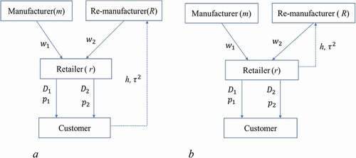
The requests for products 1 and 2 are stated below:

$D_1={\alpha }_1-{\beta }_p{p}_1+{\gamma }_p{p}_2$

$D_2={\alpha }_2-{\beta }_p{p}_2+{\gamma }_p{p}_1$

$D_b={\alpha }_b-{\beta }_b{p}_b$

4.2. Direct collection

Here, old used products are purchased directly from the consumer by the remanufacturer. This process does not engage the services of middlemen. The payment flow in a direct collection is shown in Figure 1a. The profit function of the remanufacturer, manufacturer, and retailer, in the case of direct collection is shown below:

(4.1) ${{\pi }_R}^{dn}=D_2\left(w_2-c_m+\mathrm{\Delta }\tau \right)-\frac{A{\tau }^2}{2}$(4.1)

Subject to

$0\le \tau \le 1$

(4.2) ${{\pi }_m}^{dn}=D_1\left(w_1-c_m\right)$(4.2)

(4.3) ${{\pi }_r}^{dn}=D_1\left(p_1-w_1-c_1\right)+D_2\left(p_2-w_2-c_2\right)$(4.3)

Subject to

$p_1\ge w_1\mathrm{a}\mathrm{n}\mathrm{d}{p}_2\ge w_2$

The first term in the objective function of the remanufacturer (see equation 1) is the gross income from the refurbished products. The second term indicates refurbishing cost, the third term represents saving production cost by utilising old used products, and the last term represents the cost incurred to collect the used products.

In the manufacturer’s objective function (see equation 2), the first term is the sales revenue from new products, and the last term is the production cost of new products.

In the retailer’s objective function (see equation 3), the first term represents the sales profit obtained from new products and the second term indicates the sales profit from refurbished products.

Here, the backward induction method was applied to determine the optimal value of the selling price, collection effort and wholesale price. Therefore, the manufacturer and remanufacturer should take the retailer’s reaction function into account when considering their respective price decisions. Here, the retailer’s reaction function, given wholesale prices $w_1$and$w_2$, can be derived from the first-order condition of (4.3).

(4.4) $\underset{p_i,p_j}{p_i{p}_j\in \mathrm{a}\mathrm{r}\mathrm{g}\mathrm{m}\mathrm{a}\mathrm{x}}{\pi }_r^{dn}(p_i,p_j|w_i,w_j,\tau )i,j=1,2,i\ne j$(4.4)

‘The objective function is concave as $\frac{{\mathrm{\partial }}^2{\pi }_r^{dn}}{\mathrm{\partial }{p_1}^2}=-2{\beta }_p$, $\frac{{\mathrm{\partial }}^2{\pi }_r^{dn}}{\mathrm{\partial }{p_2}^2}=-2{\beta }_p$ and$\frac{\mathrm{\partial }\pi {{ }_r^{dn}}^2}{\mathrm{\partial }{p}_1\mathrm{\partial }{p}_2}=2{\gamma }_p$, it is solved by the first-order condition and the value of the price and collection effort are as follows:’

(4.5) $p_1=\frac{{\alpha }_1{\beta }_p+{\alpha }_2{\gamma }_p+\left(c_1+w_1\right)\left({\beta }_p^2-{\gamma }_p^2\right)}{2\left({\beta }_p^2-{\gamma }_p^2\right)}$(4.5)

(4.6) $p_2=\frac{{\alpha }_2{\beta }_p+{\alpha }_1{\gamma }_p+\left(c_2+w_2\right)\left({\beta }_p^2-{\gamma }_p^2\right)}{2\left({\beta }_p^2-{\gamma }_p^2\right)}$(4.6)

4.3. Manufacturer’s profit

It is evident that the equilibrium of selling price and product demand is a linear function of the manufacturer’s bulk price. Here, the manufacturer’s reaction function, given selling prices $p_1$ and$p_2$, is deduced from the first-order condition of (4.2).

(4.7) $\underset{w_1}{w_1\in \mathrm{a}\mathrm{r}\mathrm{g}\mathrm{m}\mathrm{a}\mathrm{x}}{\pi }_m^{dn}(w_1|,p_1,p_2)$(4.7)

Using the reaction function Eqs. (4.5(4.5) $p_1=\frac{{\alpha }_1{\beta }_p+{\alpha }_2{\gamma }_p+\left(c_1+w_1\right)\left({\beta }_p^2-{\gamma }_p^2\right)}{2\left({\beta }_p^2-{\gamma }_p^2\right)}$(4.5) –4.6(4.6) $p_2=\frac{{\alpha }_2{\beta }_p+{\alpha }_1{\gamma }_p+\left(c_2+w_2\right)\left({\beta }_p^2-{\gamma }_p^2\right)}{2\left({\beta }_p^2-{\gamma }_p^2\right)}$(4.6) ), the manufacturers’ equilibrium wholesale price is deduced through first-order conditions and the value of the wholesale price is as follows:

(4.8) $w_1=\frac{{\alpha }_1-c_1{\beta }_p+c_m{\beta }_p+c_2{\gamma }_p+w_2{\gamma }_p}{2{\beta }_p}$(4.8)

4.4. Remanufacturer’s profit

It is evident that the equilibrium of selling price, collection effort, and demand of refurbished products are a linear function of the remanufacturer’s wholesale price. Here, the remanufacturer’s reaction function, given selling prices $p_1$and$p_2$, is deduced from the first-order condition of (4.1).

(4.9) $\underset{w_{2,},\tau }{w_2,\tau \in \mathrm{a}\mathrm{r}\mathrm{g}\mathrm{m}\mathrm{a}\mathrm{x}}{\pi }_m^{dn}(w_2,\tau |,p_1,p_2)$(4.9)

‘Since the objective function is concave as $\frac{{\mathrm{\partial }}^2{\pi }_R^{dn}}{\mathrm{\partial }{w_2}^2}=-{\beta }_p$, $\frac{{\mathrm{\partial }}^2{\pi }_R^{dn}}{\mathrm{\partial }{\tau }^2}=-A$ and$\frac{\mathrm{\partial }\pi {{ }_R^{dn}}^2}{\mathrm{\partial }{w}_2\mathrm{\partial }\tau }=-\frac{\mathrm{\Delta }{\beta }_p}{2}$’. The first-order condition is solved and the value of the prices is as follows:

(4.10) $w_1=\frac{{\alpha }_2-\left(\mathrm{\Delta }\tau +c_2-c_m\right){\beta }_p+\left(c_1+w_1\right){\gamma }_p}{2{\beta }_p}$(4.10)

(4.11) $\tau =\frac{\mathrm{\Delta }\left({\alpha }_2-\left(c_2+w_2\right){\beta }_p+\left(c_1+w_1\right){\gamma }_p\right)}{2A}$(4.11)

Solving Eqns. (4.5(4.5) $p_1=\frac{{\alpha }_1{\beta }_p+{\alpha }_2{\gamma }_p+\left(c_1+w_1\right)\left({\beta }_p^2-{\gamma }_p^2\right)}{2\left({\beta }_p^2-{\gamma }_p^2\right)}$(4.5) , 4.6(4.6) $p_2=\frac{{\alpha }_2{\beta }_p+{\alpha }_1{\gamma }_p+\left(c_2+w_2\right)\left({\beta }_p^2-{\gamma }_p^2\right)}{2\left({\beta }_p^2-{\gamma }_p^2\right)}$(4.6) , 4.8(4.8) $w_1=\frac{{\alpha }_1-c_1{\beta }_p+c_m{\beta }_p+c_2{\gamma }_p+w_2{\gamma }_p}{2{\beta }_p}$(4.8) , 4.10(4.10) $w_1=\frac{{\alpha }_2-\left(\mathrm{\Delta }\tau +c_2-c_m\right){\beta }_p+\left(c_1+w_1\right){\gamma }_p}{2{\beta }_p}$(4.10) , & 4.11)(4.11) $\tau =\frac{\mathrm{\Delta }\left({\alpha }_2-\left(c_2+w_2\right){\beta }_p+\left(c_1+w_1\right){\gamma }_p\right)}{2A}$(4.11) simultaneously, the optimal solution of ${w_1}^{\ast },{w_2}^{\ast },{p_1}^{\ast },{p_2}^{\ast },\mathrm{a}\mathrm{n}\mathrm{d}{\tau }^{\ast }$can be determined as follows:

(4.12) ${w_1}^{\ast }=\frac{2{\beta }_p\left({\alpha }_1+\left(-c_1+c_m\right){\beta }_p\right)+\left({\alpha }_2+\left(-\mathrm{\Delta }\tau +c_2+c_m\right){\beta }_p\right){\gamma }_p+c_1{\gamma }_p^2}{4{\beta }_p^2-{\gamma }_p^2}$(4.12)

(4.13) ${w_2}^{\ast }=\frac{2{\beta }_p\left({\alpha }_2-\left(\mathrm{\Delta }\tau +c_2-c_m\right){\beta }_p\right)+\left({\alpha }_1+\left(c_1+c_m\right){\beta }_p\right){\gamma }_p+c_2{\gamma }_p^2}{4{\beta }_p^2-{\gamma }_p^2}$(4.13)

(4.14) $\begin{array}{rl}& {p_1}^{\ast }=\\ & \frac{2{\beta }_p^3\left(3{\alpha }_1+\left(c_1+c_m\right){\beta }_p\right)+{\beta }_p^2\left(5{\alpha }_2+\left(-\mathrm{\Delta }\tau +c_2+c_m\right){\beta }_p\right){\gamma }_p-{\beta }_p\left(3{\alpha }_1+2\left(c_1+c_m\right){\beta }_p\right){\gamma }_p^2-\left(2{\alpha }_2+\left(-\mathrm{\Delta }\tau +c_2+c_m\right){\beta }_p\right){\gamma }_p^3}{2\left(4{\beta }_p^4-5{\beta }_p^2{\gamma }_p^2+{\gamma }_p^4\right)}\end{array}$(4.14)

(4.15) ${p_2}^{\ast }=\frac{2{\beta }_p^3\left(3{\alpha }_2+\left(-\mathrm{\Delta }\tau +c_2+c_m\right){\beta }_p\right)+{\beta }_p^2\left(5{\alpha }_1+\left(c_1+c_m\right){\beta }_p\right){\gamma }_p+{\beta }_p\left(-3{\alpha }_2+2\left(\mathrm{\Delta }\tau -c_2-c_m\right){\beta }_p\right){\gamma }_p^2-\left(2{\alpha }_1+\left(c_1+c_m\right){\beta }_p\right){\gamma }_p^3}{2\left(4{\beta }_p^4-5{\beta }_p^2{\gamma }_p^2+{\gamma }_p^4\right)}$(4.15)

(4.16) ${\tau }^{\ast }=\frac{\mathrm{\Delta }{\beta }_p\left(2{\beta }_p\left({\alpha }_2+\left(\mathrm{\Delta }\tau -c_2-c_m\right){\beta }_p\right)+\left({\alpha }_1+\left(c_1+c_m\right){\beta }_p\right){\gamma }_p+\left(-\mathrm{\Delta }\tau +c_2+c_m\right){\gamma }_p^2\right)}{8A{\beta }_p^2-2A{\gamma }_p^2}$(4.16)

Finally, the demand for new and refurbished products can be determined as:

(4.17) $D_1={\alpha }_1-{\beta }_p{p_1}^{\ast }+{\gamma }_p{p_2}^{\ast }$(4.17)

(4.18) $D_2={\alpha }_2-{\beta }_p{p_2}^{\ast }+{\gamma }_p{p_1}^{\ast }$(4.18)

4.5. Indirect collection (In)

In this model, the remanufacturer asks the retailer to purchase used products at a specific price and then sell at a fixed transfer price to the remanufacturer h. Figure 1b. displays the payment flow in an indirect collection. The objective function of the manufacturer, remanufacturer, and retailer under a direct collection are as follows:

(4.19) ${{\pi }_m}^{In}=D_1\left(w_1-c_m\right)$(4.19)

(4.20) ${{\pi }_R}^{In}=D_2\left(w_2-c_m+\left(\mathrm{\Delta }-h\right)\tau \right)$(4.20)

(4.21) ${{\pi }_r}^{In}=D_1\left(p_1-w_1-c_1\right)+D_2\left(p_2-w_2-c_2+h\tau \right)-\frac{A{\tau }^2}{2}$(4.21)

Subject to

$p_1\ge w_1\mathrm{a}\mathrm{n}\mathrm{d}{p}_2\ge w_2$

$0\le \tau \le 1$

Here, the backward induction method was applied to ascertain the ideal value of selling price, collection effort and wholesale price. Therefore, the manufacturer and remanufacturer should take the retailer’s reaction function into account when considering their separate price decisions. Here, the retailer’s reaction function, given wholesale prices $w_1$and$w_2$, is deduced from the first-order condition of (4.21).

(4.22) $\underset{p_1,p_2,\tau }{p_{1,}{p}_2,\tau \in \mathrm{a}\mathrm{r}\mathrm{g}\mathrm{m}\mathrm{a}\mathrm{x}}{\pi }_r^{In}(p_1,p_2,\tau |w_1,w_2)$(4.22)

Appendix A shows that the objective function is naturally concave. Thus, it is solved by the first-order condition and the value of the price and collection effort are as follows:

(4.23) $p_1=\frac{{\alpha }_1{\beta }_p+{\alpha }_2{\gamma }_p+\left(c_1+w_1\right)\left({\beta }_p^2-{\gamma }_p^2\right)}{2\left({\beta }_p^2-{\gamma }_p^2\right)}$(4.23)

(4.24) $p_2=\frac{1}{4}\left(\frac{4A\left(c_2+w_2\right)-2h^2{\alpha }_2}{2A-h^2{\beta }_p}+\frac{{\alpha }_1+{\alpha }_2}{{\beta }_p-{\gamma }_p}+\frac{2h^2\left(c_1+w_1\right){\gamma }_p}{-2A+h^2{\beta }_p}+\frac{-{\alpha }_1+{\alpha }_2}{{\beta }_p+{\gamma }_p}\right)$(4.24)

(4.25) $\tau =\frac{h\left({\alpha }_2-\left(c_2+w_2\right){\beta }_p+\left(c_1+w_1\right){\gamma }_p\right)}{2A-h^2{\beta }_p}$(4.25)

4.6. Manufacturer’s profit

‘Here, the equilibrium of selling price, and demand of new product are a linear function of the producer’s bulk price. The manufacturer’s reaction function can be determined, given selling prices $p_1$and $p_2$can be derived from the first-order condition of (4.19).’

(4.26) $\underset{w_1}{w_1\in \mathrm{a}\mathrm{r}\mathrm{g}\mathrm{m}\mathrm{a}\mathrm{x}}{\pi }_m^{In}(w_1|,p_1,p_2)$(4.26)

Also, Appendix B shows that the objective function is naturally concave. Using Eqs. (4.23(4.23) $p_1=\frac{{\alpha }_1{\beta }_p+{\alpha }_2{\gamma }_p+\left(c_1+w_1\right)\left({\beta }_p^2-{\gamma }_p^2\right)}{2\left({\beta }_p^2-{\gamma }_p^2\right)}$(4.23) –4.24(4.24) $p_2=\frac{1}{4}\left(\frac{4A\left(c_2+w_2\right)-2h^2{\alpha }_2}{2A-h^2{\beta }_p}+\frac{{\alpha }_1+{\alpha }_2}{{\beta }_p-{\gamma }_p}+\frac{2h^2\left(c_1+w_1\right){\gamma }_p}{-2A+h^2{\beta }_p}+\frac{-{\alpha }_1+{\alpha }_2}{{\beta }_p+{\gamma }_p}\right)$(4.24) ), the manufacturers’ equilibrium wholesale price can be derived through first-order conditions and the value of wholesale price is as follows:

(4.27) $w_1=\frac{1}{2}\left(-c_1+c_m+\frac{{\alpha }_1\left(2A-h^2{\beta }_p\right)+\left(2A\left(c_2+w_2\right)-h^2{\alpha }_2\right){\gamma }_p}{2A{\beta }_p-h^2{\beta }_p^2+h^2{\gamma }_p^2}\right)$(4.27)

4.7. Remanufacturer’s profit

‘It was observed that the equilibrium of selling price and demand of refurbished product are a linear function of the remanufacturer’s wholesale price. Here, the remanufacturer’s reaction function, given selling prices $p_1$, $p_2$, and τ can be derived from the first-order condition of (4.20).’

(4.28) $\underset{\hspace{0.17em}{w}_{2,},\tau }{w_2\in \mathrm{a}\mathrm{r}\mathrm{g}\mathrm{m}\mathrm{a}\mathrm{x}}{\pi }_m^{dn}(w_2,\tau |,p_1,p_2)$(4.28)

‘Using Eqs.(4.23(4.23) $p_1=\frac{{\alpha }_1{\beta }_p+{\alpha }_2{\gamma }_p+\left(c_1+w_1\right)\left({\beta }_p^2-{\gamma }_p^2\right)}{2\left({\beta }_p^2-{\gamma }_p^2\right)}$(4.23) –4.25(4.25) $\tau =\frac{h\left({\alpha }_2-\left(c_2+w_2\right){\beta }_p+\left(c_1+w_1\right){\gamma }_p\right)}{2A-h^2{\beta }_p}$(4.25) ), the remanufacturers’ equilibrium wholesale price can be derived through the first-order conditions and the value of the wholesale price is as follows:’

(4.29) $w_2=\frac{{\alpha }_2\left(-2A-h\left(h-2\mathrm{\Delta }\right){\beta }_p\right)+{\beta }_p\left(2A\left(c_2-c_m\right)+h\left(\left(h-2\mathrm{\Delta }\right)c_2+h{c}_m\right){\beta }_p\right)-\left(c_1+w_1\right)\left(2A+h\left(h-2\mathrm{\Delta }\right){\beta }_p\right){\gamma }_p}{2{\beta }_p\left(-2A+h\mathrm{\Delta }{\beta }_p\right)}$(4.29)

Solving Eqns. (4.23(4.23) $p_1=\frac{{\alpha }_1{\beta }_p+{\alpha }_2{\gamma }_p+\left(c_1+w_1\right)\left({\beta }_p^2-{\gamma }_p^2\right)}{2\left({\beta }_p^2-{\gamma }_p^2\right)}$(4.23) , 4.24(4.24) $p_2=\frac{1}{4}\left(\frac{4A\left(c_2+w_2\right)-2h^2{\alpha }_2}{2A-h^2{\beta }_p}+\frac{{\alpha }_1+{\alpha }_2}{{\beta }_p-{\gamma }_p}+\frac{2h^2\left(c_1+w_1\right){\gamma }_p}{-2A+h^2{\beta }_p}+\frac{-{\alpha }_1+{\alpha }_2}{{\beta }_p+{\gamma }_p}\right)$(4.24) , 4.25(4.25) $\tau =\frac{h\left({\alpha }_2-\left(c_2+w_2\right){\beta }_p+\left(c_1+w_1\right){\gamma }_p\right)}{2A-h^2{\beta }_p}$(4.25) , 4.27(4.27) $w_1=\frac{1}{2}\left(-c_1+c_m+\frac{{\alpha }_1\left(2A-h^2{\beta }_p\right)+\left(2A\left(c_2+w_2\right)-h^2{\alpha }_2\right){\gamma }_p}{2A{\beta }_p-h^2{\beta }_p^2+h^2{\gamma }_p^2}\right)$(4.27) , & 4.29)(4.29) $w_2=\frac{{\alpha }_2\left(-2A-h\left(h-2\mathrm{\Delta }\right){\beta }_p\right)+{\beta }_p\left(2A\left(c_2-c_m\right)+h\left(\left(h-2\mathrm{\Delta }\right)c_2+h{c}_m\right){\beta }_p\right)-\left(c_1+w_1\right)\left(2A+h\left(h-2\mathrm{\Delta }\right){\beta }_p\right){\gamma }_p}{2{\beta }_p\left(-2A+h\mathrm{\Delta }{\beta }_p\right)}$(4.29) simultaneously, the ideal solution of ${w_1}^{\ast },{w_2}^{\ast },{p_1}^{\ast },{p_2}^{\ast },\mathrm{a}\mathrm{n}\mathrm{d}{\tau }^{\ast }$can be determined. Then, the request for new and refurbished products can be determined by considering the ideal price and collection effort.

Proposition 1: Under the individual pricing model, as transfer price, h, increases, the collection effort $\tau$, also increases.

Proof of Proposition 1: See Appendix

From Proposition 1, it is clear that the collection of used products will increase, as the incentive increases. This shows that when transfer price h increases, the retailer will collect more used products from the market and then decrease the refurbishing cost. This is because once consumers start receiving higher incentives, they will become more interested in returning their used items in good condition. Consequently, the competition between the manufacturer’s and remanufacturer’s products will increase.

4.8. Pure bundling model

In this model, the retailer packages new products and refurbished products into one product, which is sold at price $p_b$ by the retailer. Here, retailer can combine items that substitute each other, such as a pair of fashionable products with same or different colour or pair of healthcare products (Gurgur 2013; Wang et al. 2014). This is an example of the pure bundling scenario. The packaged product has a price lower than the sum of the individual retail prices, i.e. p_b<p₁ + p₂. Figure 2 shows the structure of the pure bundling model.

Figure 2. Pure bundling model under direct collection 2.b. Pure bundling model under indirect collection

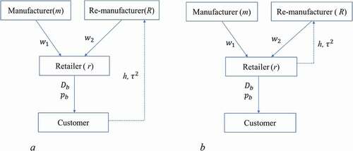
The demands of Products 1 and 2 are given as follows:

$D_b={\alpha }_p-{\beta }_b{p}_b$

4.9. Direct collection

Here, the remanufacturer buys old used products from the market without any intermediary. Figure 2a illustrates cash flow in a direct collection. The objective function of the remanufacturer, manufacturer, and retailer under direct collection are shown below:

(4.30) ${{\pi }_R}^{db}=D_b\left(w_2-c_m+\mathrm{\Delta }\tau \right)-\frac{A{\tau }^2}{2}$(4.30)

Subject to

$0\le \tau \le 1$

(4.31) ${{\pi }_m}^{db}=D_b\left(w_1-c_m\right)$(4.31)

(4.32) ${{\pi }_r}^{db}=D_b\left(p_b-w_1-w_2-c_b\right)$(4.32)

Subject to

$p_b\ge w_1,w_2$

$p_b\le p_1+p_2$

The first term in the objective function of the remanufacturer (see equation 4.30(4.30) ${{\pi }_R}^{db}=D_b\left(w_2-c_m+\mathrm{\Delta }\tau \right)-\frac{A{\tau }^2}{2}$(4.30) ), is the selling revenue obtained from the refurbished items. The second word shows the cost of purchasing the products used.

“In the producer’s objective functions (see equation 4.31(4.31) ${{\pi }_m}^{db}=D_b\left(w_1-c_m\right)$(4.31) ), the first term is the sales revenue obtained from new products, and the last term is the production cost of new products.

In the retailer’s objective function (see equation 4.32(4.32) ${{\pi }_r}^{db}=D_b\left(p_b-w_1-w_2-c_b\right)$(4.32) ), the first term represents the sales profit obtained from bundling products. The second and third terms indicate the bulk price of new and refurbished products. The last term indicates the cost incurred (repacking, packaging, and sorting, etc.) during bundling by the retailer”.

‘Here, the backward induction method was applied to determine the ideal value of selling price, collection effort and wholesale price. Therefore, the manufacturer and remanufacturer should take the retailer’s reaction function into account when considering their separate price decisions. Here, the retailer’s reaction function, given wholesale prices $w_1$and$w_2$ can be derived from the first-order condition of (4.32).’

$\underset{p_b}{p_b\in \mathrm{a}\mathrm{r}\mathrm{g}\mathrm{m}\mathrm{a}\mathrm{x}}{\pi }_r^{db}\left(p_b|w_1,w_2,\tau \right)\hspace{0.17em}\left(4.33\right)$

Since the objective function is naturally concave and is solved by the first-order condition, the value of the prices are as follows (see Appendix C):

(4.34) ${p_b}^{db}=\frac{1}{2}\left(c_b+w_1+w_2+\frac{{\alpha }_b}{{\beta }_b}\right)$(4.34)

4.10. Manufacturer’s profit

‘Here, the equilibrium of bundling price, and demand of new product are a linear function of the producer’s bulk price. We can determine the manufacturer’s reaction function, given the selling price $p_b$, can be deduced from the Eqs(4.31).’

(4.35) $\underset{w_1}{w_1\in \mathrm{a}\mathrm{r}\mathrm{g}\mathrm{m}\mathrm{a}\mathrm{x}}{\pi }_m^{db}(w_1|p_b)$(4.35)

‘Here the objective function is concave. Taking Eqn. (4.35(4.35) $\underset{w_1}{w_1\in \mathrm{a}\mathrm{r}\mathrm{g}\mathrm{m}\mathrm{a}\mathrm{x}}{\pi }_m^{db}(w_1|p_b)$(4.35) ), the manufacturers’ equilibrium wholesale price can be derived through first-order conditions and the wholesale price value as follows (See Appendix D):’

(4.36) ${w_1}^{db}=\frac{{\alpha }_b-c_b{\beta }_b+c_m{\beta }_b-w_2{\beta }_b}{2{\beta }_b}$(4.36)

4.11. Remanufacturer’s profit

‘It can be seen that the ideal selling price, collection effort, and demand of refurbished products are a linear function of the remanufacturer’s wholesale price. Here, the remanufacturer’s reaction function, given a selling price $p_b$ can be derived from the first-order condition of (4.30).’”

(4.37) $\underset{w_{2,},\tau }{w_2,\tau \in \mathrm{a}\mathrm{r}\mathrm{g}\mathrm{m}\mathrm{a}\mathrm{x}}{\pi }_m^{db}(w_2,\tau |p_b)$(4.37)

The objective function is naturally concave (See Appendix E) and is solved by the first-order condition, the value of prices are as follows:

(4.38) ${\tau }^{db}=\frac{\mathrm{\Delta }\left({\alpha }_b-\left(c_b+c_m+w_1\right){\beta }_b\right)}{4A-{\mathrm{\Delta }}^2{\beta }_b}$(4.38)

(4.39) ${w_2}^{db}=\frac{1}{2}\left(-2\left(c_b+w_1\right)+\frac{{\alpha }_b}{{\beta }_b}+\frac{4A\left(c_b+c_m+w_1\right)-{\mathrm{\Delta }}^2{\alpha }_b}{4A-{\mathrm{\Delta }}^2{\beta }_b}\right)$(4.39)

Solving Eqns. (4.34(4.34) ${p_b}^{db}=\frac{1}{2}\left(c_b+w_1+w_2+\frac{{\alpha }_b}{{\beta }_b}\right)$(4.34) , 4.36(4.36) ${w_1}^{db}=\frac{{\alpha }_b-c_b{\beta }_b+c_m{\beta }_b-w_2{\beta }_b}{2{\beta }_b}$(4.36) , 4.38(4.38) ${\tau }^{db}=\frac{\mathrm{\Delta }\left({\alpha }_b-\left(c_b+c_m+w_1\right){\beta }_b\right)}{4A-{\mathrm{\Delta }}^2{\beta }_b}$(4.38) , & 4.39)(4.39) ${w_2}^{db}=\frac{1}{2}\left(-2\left(c_b+w_1\right)+\frac{{\alpha }_b}{{\beta }_b}+\frac{4A\left(c_b+c_m+w_1\right)-{\mathrm{\Delta }}^2{\alpha }_b}{4A-{\mathrm{\Delta }}^2{\beta }_b}\right)$(4.39) simultaneously, the optimal solution of ${w_1}^{db\ast },{w_2}^{db\ast },{p_b}^{db\ast },\mathrm{a}\mathrm{n}\mathrm{d}{\tau }^{db\ast }$can be determined as follows:

(4.40) ${w_1}^{db\ast }=\frac{-2A{\alpha }_b+{\beta }_b\left(2A{c}_b+c_m\left(-2A+{\mathrm{\Delta }}^2{\beta }_b\right)\right)}{{\beta }_b\left(-6A+{\mathrm{\Delta }}^2{\beta }_b\right)}$(4.40)

(4.41) ${w_2}^{db\ast }=\frac{1}{3}\left(-3\left(c_b+c_m\right)+\frac{{\alpha }_b}{{\beta }_b}+\frac{12A\left(c_b+2c_m\right)-2{\mathrm{\Delta }}^2{\alpha }_b}{6A-{\mathrm{\Delta }}^2{\beta }_b}\right)$(4.41)

(4.42) ${p_b}^{db\ast }=\frac{-A\left(c_b+2c_m\right){\beta }_b+{\alpha }_b\left(-5A+{\mathrm{\Delta }}^2{\beta }_b\right)}{{\beta }_b\left(-6A+{\mathrm{\Delta }}^2{\beta }_b\right)}$(4.42)

(4.43) ${\tau }^{db\ast }=\frac{\mathrm{\Delta }\left({\alpha }_b-\left(c_b+2c_m\right){\beta }_b\right)}{6A-{\mathrm{\Delta }}^2{\beta }_b}$(4.43)

4.12. Indirect collection model

In this sub-section model, the reseller gathers used products from the end-consumer at a certain price and then sells them to the remanufacturer at a fixed transfer price h in Figure 2b. The objective function of the manufacturer, remanufacturer, and retailer under indirect collection is given as follows:

(4.44) ${{\pi }_m}^{Ib}=D_b\left(w_1-c_m\right)$(4.44)

(4.45) ${{\pi }_R}^{Ib}=D_b\left(w_2-c_m+\left(\mathrm{\Delta }-h\right)\tau \right)$(4.45)

(4.46) ${{\pi }_r}^{Ib}=D_b\left(p_b{-}_1-w_2-c_b+h\tau \right)-\frac{A{\tau }^2}{2}$(4.46)

Subject to

$p_b\ge w_1,w_2$

$p_b\le p_1+p_2$

$0\le \tau \le 1$

‘Here, the backward induction method was applied to explore the ideal value of selling price, collection effort and bulk price. Therefore, the manufacturer and remanufacturer should take the retailer’s reaction function into account, when considering their separate price decisions. Here, the retailer’s reaction function, given wholesale prices $w_1$and$w_2$can be deduced from Eqn. (4.46)’.

(4.47) $\underset{p_b,\tau }{p_b,\tau \in \mathrm{a}\mathrm{r}\mathrm{g}\mathrm{m}\mathrm{a}\mathrm{x}}{\pi }_r^{Ib}\left(p_b,\tau |w_1,w_2\right)$(4.47)

‘Since the objective function is concave in nature as presented in Appendix F. It is solved by the first-order condition and the value of the price and collection effort are as follows:’

(4.48) ${p_b}^{Ib}=\frac{-A\left(c_b+w_1+w_2\right){\beta }_b+{\alpha }_b\left(-A+h^2{\beta }_b\right)}{{\beta }_b\left(-2A+h^2{\beta }_b\right)}$(4.48)

(4.49) ${\tau }^{Ib}=\frac{h\left({\alpha }_b-\left(c_b+w_1+w_2\right){\beta }_b\right)}{2A-h^2{\beta }_b}$(4.49)

4.13. Manufacturer’s profit

Here, the equilibrium of bundling price, and demand of new product are a linear function of the manufacturer’s wholesale price. We can determine the manufacturer’s reaction function, given that a selling price $p_b$ can be derived from the Eqs(4.44(4.44) ${{\pi }_m}^{Ib}=D_b\left(w_1-c_m\right)$(4.44) ).

(4.50) $\underset{w_1}{w_1\in \mathrm{a}\mathrm{r}\mathrm{g}\mathrm{m}\mathrm{a}\mathrm{x}}{\pi }_m^{Ib}(w_1|p_b)$(4.50)

‘Since the objective function Eqn. (4.44(4.44) ${{\pi }_m}^{Ib}=D_b\left(w_1-c_m\right)$(4.44) ) is naturally concave with $w_1;$ the manufacturer’s equilibrium bulk price can be derived through first-order conditions and the value of the bulk price is as follows:’

(4.51) ${w_1}^{Ib}=\frac{1}{2}\left(-c_b+c_m-w_2+\frac{{\alpha }_b}{{\beta }_b}\right)$(4.51)

4.14. Remanufacturer’s profit

Here, the equilibrium of bundling price, collection effort, and demand of new product are linear function of the manufacturer’s wholesale price.

The producer’s reaction function can be determined, given a selling price $p_b$ and τ can be derived from Eqs.(4.45(4.45) ${{\pi }_R}^{Ib}=D_b\left(w_2-c_m+\left(\mathrm{\Delta }-h\right)\tau \right)$(4.45) ).

(4.52) $\underset{w_{2,}}{w_2\in \mathrm{a}\mathrm{r}\mathrm{g}\mathrm{m}\mathrm{a}\mathrm{x}}{\pi }_m^{db}(w_2|\tau ,p_b)$(4.52)

Since the objective function is naturally concave as presented in Appendix G, it is determined by the first-order condition and the value of prices as follows:

(4.53) ${w_2}^{Ib}=\frac{{\alpha }_b\left(-2A-h\left(h-2\mathrm{\Delta }\right){\beta }_b\right)+{\beta }_b\left(2A\left(c_b-c_m+w_1\right)+h\left(\left(h-2\mathrm{\Delta }\right)c_b+h{c}_m+\left(h-2\mathrm{\Delta }\right)w_1\right){\beta }_b\right)}{2{\beta }_b\left(-2A+h\mathrm{\Delta }{\beta }_b\right)}$(4.53)

Solving Eqns. (4.49(4.49) ${\tau }^{Ib}=\frac{h\left({\alpha }_b-\left(c_b+w_1+w_2\right){\beta }_b\right)}{2A-h^2{\beta }_b}$(4.49) , 4.50(4.50) $\underset{w_1}{w_1\in \mathrm{a}\mathrm{r}\mathrm{g}\mathrm{m}\mathrm{a}\mathrm{x}}{\pi }_m^{Ib}(w_1|p_b)$(4.50) , 4.52(4.52) $\underset{w_{2,}}{w_2\in \mathrm{a}\mathrm{r}\mathrm{g}\mathrm{m}\mathrm{a}\mathrm{x}}{\pi }_m^{db}(w_2|\tau ,p_b)$(4.52) , & 4.54)(4.54) ${w_1}^{Ib\ast }=\frac{{\alpha }_b\left(-2A+h^2{\beta }_b\right)+{\beta }_b\left(2A\left(c_b-c_m\right)-h\left(h{c}_b+\left(h-2\mathrm{\Delta }\right)c_m\right){\beta }_b\right)}{{\beta }_b\left(-6A+h\left(h+2\mathrm{\Delta }\right){\beta }_b\right)}$(4.54) simultaneously, the optimal solution of ${w_1}^{Ib\ast },{w_2}^{Ib\ast },{p_b}^{Ib\ast },\mathrm{a}\mathrm{n}\mathrm{d}{\tau }^{Ib\ast }$can be determined as follows:

(4.54) ${w_1}^{Ib\ast }=\frac{{\alpha }_b\left(-2A+h^2{\beta }_b\right)+{\beta }_b\left(2A\left(c_b-c_m\right)-h\left(h{c}_b+\left(h-2\mathrm{\Delta }\right)c_m\right){\beta }_b\right)}{{\beta }_b\left(-6A+h\left(h+2\mathrm{\Delta }\right){\beta }_b\right)}$(4.54)

(4.55) ${w_2}^{Ib\ast }=\frac{-{\alpha }_b\left(2A+h\left(h-2\mathrm{\Delta }\right){\beta }_b\right)+{\beta }_b\left(c_b\left(2A+h\left(h-2\mathrm{\Delta }\right){\beta }_b\right)+c_m\left(-2A+h\left(3h-2\mathrm{\Delta }\right){\beta }_b\right)\right)}{{\beta }_b\left(-6A+h\left(h+2\mathrm{\Delta }\right){\beta }_b\right)}$(4.55)

(4.56) ${\tau }^{Ib\ast }=\frac{h\left({\alpha }_b-\left(c_b+2c_m\right){\beta }_b\right)}{6A-h\left(h+2\mathrm{\Delta }\right){\beta }_b}$(4.56)

(4.57) ${p_b}^{Ib\ast }=\frac{-A\left(c_b+2c_m\right){\beta }_b+{\alpha }_b\left(-5A+h\left(h+2\mathrm{\Delta }\right){\beta }_b\right)}{{\beta }_b\left(-6A+h\left(h+2\mathrm{\Delta }\right){\beta }_b\right)}$(4.57)

The demands of pure bundling product is given as follows:

$D_p={\alpha }_p-{\beta }_b{p_b}^{Ib\ast }$

4.15. Mixed bundling model

The individual pricing model provides new and refurbished products separately, and in the case of pure bundling, it offers only the bundled products, whereas the mixed bundling case offers both bundled and component product(s) individually (Zhou, Song, and Gavirneni 2020). Here, the retailer can package new and refurbished products together with his private label product at a bundle price $p_b$. Figure 3 describes the framework.

Figure 3. A. Mixed bundling model under direct collection. b. Mixed bundling model under indirect collection

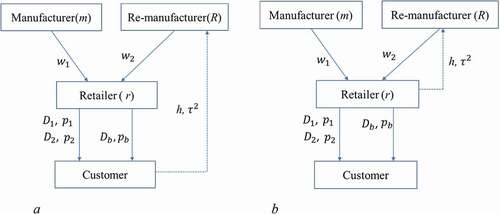
The demand for the new product, refurbished product, and bundle product is as follows:

(4.57a) ${D_1}^M={\alpha }_1-{\beta }_p{p}_1+{\gamma }_p{p}_2+{\mu }_1{p}_b$(4.57a)

(4.57b) ${D_2}^M={\alpha }_2-{\beta }_p{p}_2+{\gamma }_p{p}_1+{\mu }_2{p}_b$(4.57b)

(4.57c) ${D_b}^M={\alpha }_b-{\beta }_b{p}_b+{\mu }_1{p}_1+{\mu }_2{p}_2$(4.57c)

It is found that similar types of demand function also have been addressed in the previous literature (Ma and Mallik 2017; Pan and Zhou 2017; Jena & Ghadge 2020; Guo et al. 2021).

4.16. Direct collection

‘Here, the used product is directly collected by the remanufacturer from the market. Figure 3a. reflects the flow of payments in a direct collection. The objective function of the remanufacturer, manufacturer, and retailer under direct collection are given as follows:’

(4.58) ${{\pi }_R}^{dM}=\left(w_2-c_m+\mathrm{\Delta }\tau \right)\left({D_2}^M+{D_b}^M\right)-\frac{A{\tau }^2}{2}$(4.58)

$0\le \tau \le 1$

(4.59) ${{\pi }_m}^{dM}=\left(w_1-c_m\right)\left({D_1}^M+{D_b}^M\right)$(4.59)

(4.60) ${{\pi }_r}^{dM}=\left(p_b-w_1-w_2-c_b\right){D_b}^M+\left(p_1-w_1-c_1\right){D_1}^M+\left(p_2-w_2-c_2\right){D_2}^M$(4.60)

Subject to

$p_1\ge w_1\mathrm{a}\mathrm{n}\mathrm{d}{p}_2\ge w_2$

$p_b\ge p_1+p_2$

Here, we have identified the optimal value of selling price, collection effort and wholesale price through the backward induction method. Therefore, the manufacturer and remanufacturer consider the retailer’s reaction function for their respective price decisions. Here, retailer reaction function, given a wholesale price ${w_1}^{dM}$and${w_2}^{dM}$ can be derived from the Eqn. (4.60(4.60) ${{\pi }_r}^{dM}=\left(p_b-w_1-w_2-c_b\right){D_b}^M+\left(p_1-w_1-c_1\right){D_1}^M+\left(p_2-w_2-c_2\right){D_2}^M$(4.60) ).

(4.61) $\underset{\hspace{0.17em}{p}_b,p_1,p_2}{p_b,p_1,p_2\in \mathrm{a}\mathrm{r}\mathrm{g}\mathrm{m}\mathrm{a}\mathrm{x}}{\pi }_r^{dM}(p_b,p_1,p_2|w_1,w_2,\tau )$(4.61)

‘The objective function is concave (See Appendix H) and is solved by the first-order condition, the value of prices are as follows:’

(4.62) ${p_1}^{dM}=\frac{{\alpha }_1+c_1{\beta }_p+w_1{\beta }_p+\frac{{\alpha }_b{\beta }_p\left({\beta }_p{\mu }_1+{\gamma }_p{\mu }_2\right)+{\alpha }_2{\beta }_p\left({\beta }_b{\gamma }_p+{\mu }_1{\mu }_2\right)+{\alpha }_1\left({\beta }_b{\gamma }_p^2+{\beta }_p{\mu }_1^2+2{\gamma }_p{\mu }_1{\mu }_2\right)}{{\beta }_b\left({\beta }_p^2-{\gamma }_p^2\right)-2{\gamma }_p{\mu }_1{\mu }_2-{\beta }_p\left({\mu }_1^2+{\mu }_2^2\right)}}{2{\beta }_p}$(4.62)

(4.63) ${p_2}^{dM}=\frac{1}{2}\left(c_2+w_2+\frac{{\alpha }_2\left({\beta }_b{\beta }_p-{\mu }_1^2\right)+{\alpha }_b\left({\gamma }_p{\mu }_1+{\beta }_p{\mu }_2\right)+{\alpha }_1\left({\beta }_b{\gamma }_p+{\mu }_1{\mu }_2\right)}{{\beta }_b\left({\beta }_p^2-{\gamma }_p^2\right)-2{\gamma }_p{\mu }_1{\mu }_2-{\beta }_p\left({\mu }_1^2+{\mu }_2^2\right)}\right)$(4.63)

(4.64) ${p_b}^{dM}=\frac{1}{2}\left(c_b+w_1+w_2+\frac{{\alpha }_b\left({\beta }_p^2-{\gamma }_p^2\right)+{\alpha }_2\left({\gamma }_p{\mu }_1+{\beta }_p{\mu }_2\right)+{\alpha }_1\left({\beta }_p{\mu }_1+{\gamma }_p{\mu }_2\right)}{{\beta }_b\left({\beta }_p^2-{\gamma }_p^2\right)-2{\gamma }_p{\mu }_1{\mu }_2-{\beta }_p\left({\mu }_1^2+{\mu }_2^2\right)}\right)$(4.64)

4.17. Manufacturer’s profit

Here, the equilibrium of bundling price and demand of new product are linear function of wholesale price by the manufacturer. We can find out manufacturer reaction function, given a selling price of price $p_b$, $p_1$,$and{p}_2$ can be derived from the Eqn. (4.59(4.59) ${{\pi }_m}^{dM}=\left(w_1-c_m\right)\left({D_1}^M+{D_b}^M\right)$(4.59) ).

(4.65) $\underset{\hspace{0.17em}{w}_1}{w_1\in \mathrm{a}\mathrm{r}\mathrm{g}\mathrm{m}\mathrm{a}\mathrm{x}}{\pi }_m^{dM}(w_1|p_{b,}{p}_1,p_2)$(4.65)

‘Since the objective function Eqn. (4.65(4.65) $\underset{\hspace{0.17em}{w}_1}{w_1\in \mathrm{a}\mathrm{r}\mathrm{g}\mathrm{m}\mathrm{a}\mathrm{x}}{\pi }_m^{dM}(w_1|p_{b,}{p}_1,p_2)$(4.65) ) is concave with $w_1$ . The manufacturers’ equilibrium wholesale price can be derived through the first-order conditions and the value of wholesale price is as follows:’

(4.66) ${w_1}^{dM}=\frac{{\alpha }_1+{\alpha }_b+c_m\left({\beta }_b+{\beta }_p-2{\mu }_1\right)+c_b\left(-{\beta }_b+{\mu }_1\right)+c_1\left(-{\beta }_p+{\mu }_1\right)+c_2\left({\gamma }_p+{\mu }_2\right)+w_2\left(-{\beta }_b+{\gamma }_p+{\mu }_1+{\mu }_2\right)}{2\left({\beta }_b+{\beta }_p-2{\mu }_1\right)}$(4.66)

4.18. Remanufacturer’s profit

We can find out manufacturer’s reaction function, given a selling price of price $p_b$ and τ can be derived from the Eqn (4.58(4.58) ${{\pi }_R}^{dM}=\left(w_2-c_m+\mathrm{\Delta }\tau \right)\left({D_2}^M+{D_b}^M\right)-\frac{A{\tau }^2}{2}$(4.58) ).

(4.67) $\underset{\hspace{0.17em}{w}_{2,},\tau }{w_{2,}\tau \in \mathrm{a}\mathrm{r}\mathrm{g}\mathrm{m}\mathrm{a}\mathrm{x}}{\pi }_m^{db}(w_2,\tau |p_{b,}{p}_1,p_2)$(4.67)

The objective function is concave (See Appendix I) and is solved by the first-order condition, and the values of prices are as follows:

(4.68) ${w_2}^{dM}=\frac{{\alpha }_2+{\alpha }_b-\left(\mathrm{\Delta }\tau +c_b-c_m+w_1\right){\beta }_b-\left(\mathrm{\Delta }\tau +c_2-c_m\right){\beta }_p+\left(c_1+w_1\right)\left({\gamma }_p+{\mu }_1\right)+\left(2\mathrm{\Delta }\tau +c_2+c_b-2c_m+w_1\right){\mu }_2}{2\left({\beta }_b+{\beta }_p-2{\mu }_2\right)}$(4.68)

(4.69) ${\tau }^{dM}=\frac{\mathrm{\Delta }\left({\alpha }_2+{\alpha }_b+c_1\left({\gamma }_p+{\mu }_1\right)-w_2\left({\beta }_b+{\beta }_p-2{\mu }_2\right)+c_b\left(-{\beta }_b+{\mu }_2\right)+c_2\left(-{\beta }_p+{\mu }_2\right)+w_1\left(-{\beta }_b+{\gamma }_p+{\mu }_1+{\mu }_2\right)\right)}{2A}$(4.69)

4. 19. Indirect collection strategy

Here, the retailer collects used product from the market and then sells these products to the retailer in Figure 3b. The objective function of the remanufacturer, manufacturer, and retailer under indirect collection are given as follows:

(4.70) ${{\pi }_R}^{IM}=\left(w_2-c_m+\left(\mathrm{\Delta }-h\right)\tau \right)\left({D_2}^M+{D_b}^M\right)$(4.70)

(4.71) ${{\pi }_m}^{IM}=\left(w_1-c_m\right)\left({D_1}^M+{D_b}^M\right)$(4.71)

(4.72) ${{\pi }_r}^{IM}=\left(p_b-w_1-w_2-c_b\right){D_b}^M+\left(p_1-w_1-c_1\right){D_1}^M+\left(p_2-w_2-c_2++h\tau \right){D_2}^M-\frac{A{\tau }^2}{2}$(4.72)

Subject to

$p_1\ge w_1\mathrm{a}\mathrm{n}\mathrm{d}{p}_2\ge w_2$

$p_b\ge p_1+p_2$

$0\le \tau \le 1$

‘Here, the manufacturer and remanufacturer take the retailer’s reaction function into the consideration of their respective price decisions. Here, retailer reaction function, given a wholesale price $w_1$and$w_2$ can be derived from the Eqn. (4.73).’

(4.73) $\underset{\hspace{0.17em}{p}_b,p_1,p_2}{p_b,p_1,p_2,\tau \in \mathrm{a}\mathrm{r}\mathrm{g}\mathrm{m}\mathrm{a}\mathrm{x}}{\pi }_r^{dM}(p_b,p_1,p_2,\tau |w_1,w_2,\tau )$(4.73)

‘Since the objective function is concave in nature as presented in Appendix J. it is solved by the first-order condition and the value of price and collection effort are as follows:’

(4.74) ${p_b}^{IM}=\frac{{\alpha }_b+c_b{\beta }_b+w_1{\beta }_b+w_2{\beta }_b-c_1{\mu }_1+2p_1{\mu }_1-w_1{\mu }_1+h\tau {\mu }_2-c_2{\mu }_2+2p_2{\mu }_2-w_2{\mu }_2}{2{\beta }_b}$(4.74)

(4.75) ${p_1}^{IM}=\frac{{\alpha }_1+c_1{\beta }_p+w_1{\beta }_p+h\tau {\gamma }_p-c_2{\gamma }_p+2p_2{\gamma }_p-w_2{\gamma }_p-c_b{\mu }_1+2p_b{\mu }_1-w_1{\mu }_1-w_2{\mu }_1}{2{\beta }_p}$(4.75)

(4.76) ${p_2}^{IM}=\frac{{\alpha }_2-h\tau {\beta }_p+c_2{\beta }_p+w_2{\beta }_p-c_1{\gamma }_p+2p_1{\gamma }_p-w_1{\gamma }_p-c_b{\mu }_2+2p_b{\mu }_2-w_1{\mu }_2-w_2{\mu }_2}{2{\beta }_p}$(4.76)

(4.77) ${\tau }^{IM}=\frac{h\left({\alpha }_2-p_2{\beta }_p+p_1{\gamma }_p+p_b{\mu }_2\right)}{A}$(4.77)

We can find out manufacturer wholesale price $w_1$ and remanufacturer’s wholesale price $w_2$, by putting the optimal value of ${p_b}^{IM}$, ${\tau }^{IM}$, ${p_1}^{IM}$,$and{p_2}^{IM}$ in the Eqn (4.70(4.70) ${{\pi }_R}^{IM}=\left(w_2-c_m+\left(\mathrm{\Delta }-h\right)\tau \right)\left({D_2}^M+{D_b}^M\right)$(4.70) ) and in Eqn. (4.71(4.71) ${{\pi }_m}^{IM}=\left(w_1-c_m\right)\left({D_1}^M+{D_b}^M\right)$(4.71) ).

Proposition 2: Under indirect collection, as the collection effort, τ, increases, the bundling price, $p_b$, increases in mixed bundling, whereas bundling price,$p_b$, decreases in pure bundling.

Proof. Proposition 2: See Appendix

‘From Proposition 2, it can be seen that the remanufacturer is always better off with a higher bundling price. The remanufacturer collects more used products, this implies that the collection cost becomes higher while the refurbishing cost becomes lower. In pure bundling, the retailer sells refurbished products through bundling with new products, and the demand for bundling products decreases. This is because of the consumer’s lower perception towards refurbished products. Therefore, the retailer maintains a lower selling price of bundling products to capture price-sensitive consumers. Whereas, in mixed bundling, the retailer sells both the bundle and component products. As a result, the retailer captures all types of consumers. Because of the competition, remanufacturers sell their products at a lower price to attract consumers, while manufacturers sell their new products at a higher price to make the differentiation. Hence, the retailer resells bundling products at a higher price compared to pure bundling.’

5. Comparison of results

The comparison of three different decision models under pure bundling and mixed bundling are presented below. A comparison has been made between all three decision models under pure and mixed bundling models.

‘Observation 1: The ordinal relationship between the optimal selling price and collection effort level considering pure and mixed bundling under direct and indirect collections are as follows:’

${p_b}^{Ib}<{p_b}^{db}<{p_b}^{dM}<{p_b}^{IM}$, Whereas: ${\tau }^{Ib}>{\tau }^{dM}>{\tau }^{IM}>{\tau }^{db}$.

‘From Observation 1, it can be seen that the equilibrium bundling retail prices are almost in-distinguishable between direct and indirect collection strategies under mixed bundling. However, in mixed bundling, the selling price of the bundle product is higher compared to pure bundling. Whereas, the bundling price is higher in direct collection strategy compared to indirect collection under the cases of pure bundling. It happens because of the lower wholesale price of the refurbished products. Again, the manufacturer sells new products with a higher price in a direct collection system compared to an indirect system. Consequently, the demand for a refurbished product increase. However, the collection effort is higher in indirect collection strategy under pure bundling compared to the other three cases. This is because of the closeness between retailers and consumers compared to remanufacturers and consumers. As a result, it creates faith between retailers and consumers’.

‘Here, the manufacturer offers a higher wholesale price for new component products and the retailer makes the bundling product from new and refurbished component products. These bundle products in mixed bundling, generate higher profit as compared to pure bundling. This implies that the retailer makes more effort to sell component products compared to only bundle products. Thus, the demand in mixed bundling is higher when compared to that of pure bundling. This is because more consumers are attracted to purchase bundled products’.

Observation 2: The profit of the remanufacturer, manufacturer, and retailer considering pure and mixed bundling under direct and indirect collections are as follows:${{\pi }_R}^{Ib}>{{\pi }_R}^{dM}>{{\pi }_R}^{IM}>{{\pi }_R}^{db}$, ${{\pi }_m}^{dM}>{{\pi }_m}^{IM}>{{\pi }_m}^{Ib}>{{\pi }_m}^{db}$, and ${{\pi }_r}^{dM}>{{\pi }_r}^{IM}>{{\pi }_r}^{Ib}>{{\pi }_r}^{db}$.

From Observation 2, the profit of the remanufacturer in indirect collection strategy under pure bundling is higher compared to all three cases. Here, the remanufacturer collects more old used products from the market through the retailer and also sells refurbished products to the retailer at a higher margin compared to direct systems, thereby increasing the gain from refurbished products. The remanufacturer’s demand decreases in the indirect collection system compared to the direct system. The retail price is mainly affected by wholesale price and a fraction of the collection rate. In addition, the retailer sells component products and bundled products simultaneously. However, the retailer’s profit is lower in pure bundling compared to the individual pricing model and mixed bundling. This implies that the perception of high-value consumers towards pure bundling is lower compared to mixed bundling, because they purchase new products only. The demand for bundling products is lower compared to the other two models. The retailer sells both bundling products and component products to high and low consumers, respectively. Consequently, it attracts more price-sensitive consumers, when purchasing bundling products. Also, the revenue attributed to the coordination can be effectively shared among the supply chain members to increase supply, demand and profits. Again, in mixed bundling, the manufacturer sells new products to the consumer at a higher price compared to pure bundling. This is because the manufacturer wants to show that new products have a better quality than refurbished products. Therefore, the profit of the manufacturer and retailer in direct collection strategy under mixed bundling is higher compared to pure bundling.

6. Numerical example

In this section, we present a numerical analysis to illustrate the working of all the three models and gain result. The values of the parameters that we have taken is as follows:$\begin{array}{rl}& {\alpha }_1=100,{\alpha }_2=50,{\beta }_p=5,\\ & {\gamma }_p=0.8,{\alpha }_b=150,{\beta }_b=5,\\ & c_m=8,c_2=1,c_1=2,c_b=3,\\ & \mathrm{\Delta }=3,h=5,A=100,\\ & {\mu }_2=0.4,{\mu }_1=0.3\end{array}$(Ma and Mallik 2017; Liu et al., 2020).

6.1. Results and discussion

‘The results of this analysis summarised in Table 3 show that the total supply chain profit is higher in mixed bundling compared to the other two models. This argument is consistent with the findings of (Vamosiu 2018; Chen, Yang, and Guo 2019). However, in their studies, they did not consider the refurbishing process under different collection strategies. This indicates the novelty of this study. The most significant observation of this study is that the total supply chain profit is higher in an indirect system compared to a direct system under pure bundling and the individual pricing model. It was observed that under mixed bundling, SC profit is higher in a direct collection system compared to an indirect collection system. This is an interesting finding, as it is contrary to what we know from previous studies (Gan et al. 2017). Furthermore, the remanufacturer and manufacturer gain more profit under the bundling model compared to the individual pricing model. This is because the lower wholesale price causes higher demand and that impacts the profit. While the profit of the retailer is higher in the individual pricing model compared to the pure bundling model. It happens because of the lower margin on used products and lower selling price. More profit is acquired in mixed bundling compared to the other two models. Similarly, it was also observed that the collection of used products is higher in bundling models compared to individual pricing models. The wholesale price of new component products is higher in individual pricing models compared to pure bundling. Whereas, the selling price of refurbished products is higher in mixed bundling compared to the individual pricing model’.

Table 3. Results by different bundling case

	Individual Pricing model		Pure bundling		Mixed bundling
Variables	Direct	Indirect	Direct	Indirect	Direct	Indirect
w1	13.84	13.65	11.96	10.53	14.16	13.51
w2	9.54	10.45	11.07	13.92	10.43	12.34
p1	19	18.91	-	-	20.39	20.06
p2	12.04	11.62	-	-	13.99	13.74
pb	-	-	28.01	26.61	30.20	30.83
τ	0.14	0.35	.29	.84	.57	.48
${\pi }_r$	53.73	55.44	19.70	21.67	126.99	120.89
${\pi }_R$	7.93	12.27	34.89	71.74	63.05	57.52
${\pi }_m$	29.89	83.35	39.03	43.01	178.92	150.46
Total profit	91.55	151.06	93.62	136.42	368.96	328.87

Under mixed bundling, the retailer utilises limited capacity and spends less on collection strategy effort to produce more bundled products. Conversely, under pure bundling, the retailer utilises limited capacity to produce less bundled products, because bundling cost significantly affects profit compared to component products. The selling price and collection effort is higher in mixed bundling and causes higher profit compared to pure bundling. Price and quality sensitive consumers prefer mixed bundling, as they have multiple options to purchase the product. It implies that consumers perceive the existence of different valuations between new and refurbished products. However, the individual pricing model approach outperforms pure bundling when the price discount is high and customers have a clear demand distinction for refurbished products.

6.2. Sensitivity analysis

Sensitivity analysis was conducted to investigate the influence of different variables on the model.

6.2.1. Market size influence

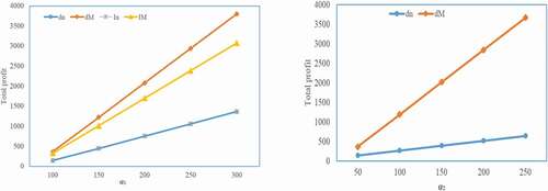
‘The impact of market size, ${\alpha }_1$ and ${\alpha }_2$on supply chain profit was studied, observing that the total profit increases, as the market size increases for all four models and two models, respectively (See Figure 4a. and Figure 4b). When market size increases, the net benefit for mixed bundling is greater than for the other two models. This happens because the retailer sells component and bundle products to the market at a higher selling price and also makes a higher collection effort in mixed bundling compared to individual pricing models. Some consumers show low interest towards refurbished products as they perceive low quality. However, in mixed bundling, retailers capture both high and low-value end consumers towards refurbished and new products by selling bundled and component products, respectively. It was also observed that the total profit in mixed bundling under direct collection system is higher compared to indirect collection models. This is because of the higher demand and absence of double marginalisation in collection. As the market size increases, the total profit in an individual system under direct and indirect systems becomes nearly equal (see Figure 4a) because there is equal bargaining power between the retailer and manufacturer. Furthermore, both the retailer and manufacturer can explore the demand in dM models compared to the other two dn and In models, because of the better service they offer to the consumers’.

Figure 4. A.Total profit of SC with different Fig.4b.Total profit for SC with different value of new product market size (α₁).” values of remanufactured market size (α₂)

6.2.2. Price elasticity influence

‘The effect of price elasticity,${\beta }_b$on supply chain profit under mixed and pure bundling systems for four models was analysed (See Figure 5a). Similarly, the impact of price elasticity,${\beta }_p$on the supply chain profit for four models under mixed bundling and individual pricing models was assessed. The results presented in Figure 5a and Figure 5b show that the total profit decreases as the value of price elasticity increases in all the cases. When ${\beta }_b$increases, the retailer’s selling price becomes higher compared with direct and indirect cases under pure bundling. This is because the retail margin of the respective products is higher compared to the other two cases and the wholesale price of new products in mixed bundling is higher compared to pure bundling. Here, the manufacturer and retailer generate more profit compared to pure bundling because in pure bundling, the retailer only captures price-sensitive consumers. However, higher selling price negatively impacts product demand and causes lower profit. One of the interesting observations is that the total profit in pure bundling under direct collection system is higher compared to the indirect system as β_b increases up to a certain threshold value 4. Thereafter, indirect systems generate higher profit compared to direct systems. It happens because the higher selling price and higher wholesale price of new and refurbished products negatively impact product demand.’

Figure 5. A.Total profit with different value of price elasticity (β_b).” b.Total profit for different value of price elasticity(β_p)

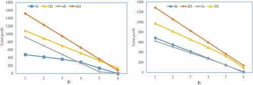
When ${\beta }_p$increases, the component’s product demand decreases but the demand of the bundling product increases, as the selling price of the bundling product is lower than the individual component price (see Figure 5b). The profit of the supply chain is higher in mixed bundling compared to the individual pricing model, although total profit decreases in both cases as ${\beta }_p$increases. The demand for bundled products will decrease as ${\beta }_p$ increases, thus leading to an increase in the total supply chain’s profit. The best option, therefore, is to maintain a mixed bundling system as compared to other systems.

6.2.3. Effects of cross-price elasticity

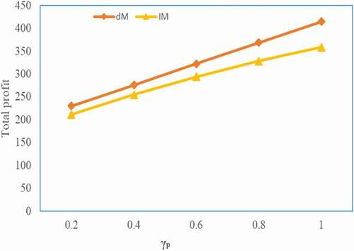
The effects of market competition γ_p on total profit for both cases are discussed here. Figure 6 shows that under direct and indirect collection systems, the total SC profit rises as market competition in mixed bundling. Due to the competition between new and refurbished products, the total profit is affected by the supply chain players. However, the total profit in mixed bundling is higher in direct collection compared to the indirect collection model. Here, the retailer sells both refurbished products and new products individually and as a bundle. Consequently, the negative effect of price competition between these two products is neutralised by increasing the bundling demand. Therefore, mixed bundling generated higher profit compared to the indirect system. The best option, therefore, is to maintain a mixed bundling system under a direct collection system.

Figure 6. Total profit for different value of cross price elasticity(γ_p)

7. Conclusion

“This research investigated the impact of pure bundling and mixed bundling considering different collection strategies under price competition in a CLSC. To the best of our knowledge, this is the first paper to formally address the issue of bundling in CLSC frameworks. Here, the optimisation decisions of the manufacturer, retailer and remanufacturer are investigated in a CLSC under price competition while considering pure and mixed bundling. Thus, this paper studied pure bundling and mixed bundling considering direct and indirect collection strategies of used products under price competition. The main findings of the study that can be used for practical implications are as follows:

• The total supply chain profit, manufacturer’s profit, and retailer’s profit are affected positively by both collection strategies. Recognising these, the manufacturer and retailer can orchestrate the CLSC to meet the supply chain objectives. This insight is the key contribution of our paper, characterising the impact of selection strategy in a two-echelon distribution channel on mixed and pure bundling.

• Among the three frameworks of the CLSCs, the individual pricing model recorded the lowest performance under direct collection, and mixed bundling had the highest performance in direct collection strategy. Whereas, pure bundling strategy had the lowest performance under indirect system compared to individual and mixed bundling strategies. This addresses research question one. It was found that the retailer, manufacturer, and remanufacturer generated higher profit in indirect collection under individual pricing and pure bundling strategy, while they generated maximum profit in mixed bundling under direct collection. This indicates that the retailer, manufacturer and remanufacturer prefer mixed bundling under direct collection, while they select individual price model and pure bundling under indirect collection strategy. This addresses research question two.

• The CLSC profit increased exponentially for all three models as market size increased. It was found that the total profit is highest in the mixed bundling model and lowest in the pure bundling model. The results show that the retailer must go for the mixed bundling strategy, irrespective of the pure and individual pricing models. This addresses research question three.

The results indicate that the operations and logistics manager will likely refuse to undertake the pure bundling strategy during price competition. Thus, considering economic gain, the manager of the manufacturing firm should disagree with the retailer for not bundling refurbished products with new products, if the collection and sales of refurbished products is unprofitable.

Our study has several limitations, which provide interesting directions for future research. First, we assumed that the manufacturer supplies substitute products to the retailer, the remanufacturer collects used products from the market, and the retailer makes bundles from the refurbished products and new products under price competition. It will be interesting to involve a third party in the collection of used products from the market and the manufacturer produces both new and refurbished products with complementary bundling (Vamosiu 2018; Ma and Mallik 2017). Second, our analysis only considered retailer bundling, incorporating manufacturer bundling could bring more insights such as secondary market platform (Vamosiu 2018; Feng et al., 219), sharing platforms (Choi et al. 2019), as well as high and low product differentiation (Chen, Yang, and Guo 2019). Third, we assumed that the cost of bundling is equal to the cost of individual component price. Nevertheless, it will be interesting to understand how the channel profit will be affected if there is uneven cost between bundling and individual cost. Last but not least, it is also interesting to investigate the customer behaviour towards combo options under the bundling. For that, it is highly recommended to refer to behaviour theories in the supply chain.

Disclosure statement

No potential conflict of interest was reported by the author(s).

Additional information

Notes on contributors

Sarat Kumar Jena

Dr. Sarat Kumar Jena is currently an Associate Professor in Operations Management at the Department of Operations management and decision science area, School of Xavier Institute of Management, Bhubaneswar, Xavier University. He has obtained Ph.D in closed-loop supply chain management, M.Tech in Industrial Engineering and Management, IIT Kharagpur, India. He has over 7 years of working experience in the industry, academia, and research. Currently Dr. Jena is an Editor of Vilakshan-XIMB Journal (Emerald Publisher). He has one experience of handling Journal as an editor and associated editor level. Dr. Jena is serving as a reviewer for more than 10 international peer reviewed journals like Decision Science, IJPE, EJOR, and Omega etc. He has conducted several training programs both nationally and internationally in the areas of supply chain management, operations management, managing experience for digital supply chain, structural equation modeling, and measurement scales design, among others. Dr. Jena has published his work in various reputable international journals such as International Journal of Production Economics, Resources, Conservation and Recycling,  Service Science (INFORMS), Sustainable Production and Consumption, Computers & Industrial Engineering, International Journal of Production Research. His research interests include value Sustainable supply chain, Circular economy research, Supply chain finance,  and Digital supply chain management. In 2018, he was selected as a researcher in the Future Talent Postdoc Career Days program at Techische Universität Darmstadt, Germany.

References

- Adams, W. J., and J. L. Yellen. 1976. “Commodity Bundling and the Burden of Monopoly.” The Quarterly Journal of Economics 90 (3): 475–498. doi:https://doi.org/10.2307/1886045.
- Agrawal, V. V., A. Atasu, and K. Van Ittersum. 2015. “Remanufacturing, Third-Party Competition, and Consumers‘ Perceived Value of New Products.” Management Science 61 (1): 60–72. doi:https://doi.org/10.1287/mnsc.2014.2099.
- Atasu, A., and G. C. Souza. 2013. “How Does Product Recovery Affect Quality Choice?” Production and Operations Management 22 (4): 991–1010. doi:https://doi.org/10.1111/j.1937-5956.2011.01290.x.
- Cao, Q., K. E. Stecke, and J. Zhang. 2015. “The Impact of Limited Supply on a Firm’s Bundling Strategy.” Production and Operations Management 24 (12): 1931–1944.
- Cao, Q., X. Geng, K. E. Stecke, and J. Zhang. 2019. “Operational Role of Retail Bundling and Its Implications in a Supply Chain.” Production and Operations Management 28 (8): 1903–1920. doi:https://doi.org/10.1111/poms.13017.
- Chen, T., F. Yang, and X. Guo. 2019. “Retailer-driven Bundling When Valuation Discount Exists.” Journal of the Operational Research Society 1 (71): 2027–2041.
- Chen, Z., S. Hong, X. Ji, R. Shi, and J. Wu. 2021. “Refurbished Products and Supply Chain Incentives.” In Annals of Operations Research, 1–21. https://doi.org/https://doi.org/10.1007/s10479-021-04016-0. (Online)
- Choi, S. C. 1991. “Price Competition in a Channel Structure with a Common Retailer.” Marketing Science 10 (4): 271–296. doi:https://doi.org/10.1287/mksc.10.4.271.
- Choi, T.-M., S. Guo, N. Liu, and X. Shi. 2019. “Values of Food Leftover Sharing Platforms in the Sharing Economy.” International Journal of Production Economics 213: 23–31. doi:https://doi.org/10.1016/j.ijpe.2019.03.005.
- Choi, Tsan-Ming, and Yongjian Li. 2015. “Sustainability in fashion business operations.„ (2015): 15400–15406.
- De Giovanni, P., and G. Zaccour. 2019. “Optimal Quality Improvements and Pricing Strategies with Active and Passive Product Returns.” Omega 88: 248–262. doi:https://doi.org/10.1016/j.omega.2018.09.007.
- De Giovanni, P., & Ramani, V. 2018. Product cannibalization and the effect of a service strategy. Journal of the operational research society, 69: 340–357.
- Dev, N. K., R. Shankar, and A. Choudhary. 2017. “Strategic Design for Inventory and Production Planning in Closed-loop Hybrid Systems.” International Journal of Production Economics 183: 345–353. doi:https://doi.org/10.1016/j.ijpe.2016.06.017.
- Feng, D., C. Shen, and Z. Pei. 2021. “Production Decisions of a Closed-loop Supply Chain considering Remanufacturing and Refurbishing under Government Subsidy.” Sustainable Production and Consumption (In Press) 27: 2058–2074. doi:https://doi.org/10.1016/j.spc.2021.04.034.
- Gan, -S.-S., I. N. Pujawan, S. Widodo, and B. Widodo. 2017. “Pricing Decision for New and remanufactured Product in a Closed-loop Supply Chain with Separate Sales-channel.” International Journal of Production Economics 190: 120–132. doi:https://doi.org/10.1016/j.ijpe.2016.08.016.
- Gayer, A., A. Aiche, and E. Gimmon. 2021. “Online Sequential Bundling: Profit Analysis and Practice.” In Electronic Commerce Research, 1–25. https://doi.org/https://doi.org/10.1007/s10660-020-09452-x. (Online)
- Genc, T. S., and P. De Giovanni. 2018. “Optimal Return and Rebate Mechanism in a Closed-loop Supply Chain Game.” European Journal of Operational Research 269 (2): 661–681. doi:https://doi.org/10.1016/j.ejor.2018.01.057.
- Ghosh, A., J. K. Jha, and S. P. Sarmah. 2016. “Optimizing a Two-echelon Serial Supply Chain with Different Carbon Policies.” International Journal of Sustainable Engineering 9 (6): 363–377. doi:https://doi.org/10.1080/19397038.2016.1195457.
- Giri, R. N., S. K. Mondal, and M. Maiti. 2020. “Bundle Pricing Strategies for Two Complementary Products with Different Channel Powers.” Annals of Operations Research 287 (2): 701–725. doi:https://doi.org/10.1007/s10479-017-2632-y.
- Girju, M., Prasad, A., and Ratchford, B. T. 2013. Pure components versus pure bundling in a marketing channel. Journal of Retailing, 89(4): 423–437.
- Guo, X., S. Zheng, Y. Yu, and F. Zhang. 2021. “Optimal Bundling Strategy for a Retail Platform under Agency Selling.” Production and Operations Management. In press https://doi.org/10.1111/poms.13366.
- Gurgur, C. Z. 2013. “Healthcare Product Procurement in Dual Supplied Systems.” IFAC Proceedings Volumes 46 (9): 1650–1655. doi:https://doi.org/10.3182/20130619-3-RU-3018.00609.
- Heydari, J., A. Heidarpoor, and A. Sabbaghnia. 2020. “Coordinated Non–monetary Sales Promotions: Buy One Get One Free Contract.” Computers & Industrial Engineering, 142: 106381.
- Jena, S. K., A. Ghadge, and S. P. Sarmah. 2018a. “Managing Channel Profit and Total Surplus in a Closed-loop Supply Chain Network.” Journal of the Operational Research Society 69 (9): 1345–1356.
- Jena, S. K., and S. P. Sarmah. 2014. “Optimal Acquisition Price Management in a Remanufacturing System.” International Journal of Sustainable Engineering 7 (2): 154–170. doi:https://doi.org/10.1080/19397038.2013.811705.
- Jena, S. K., and S. P. Sarmah. 2015. “Measurement of Consumers‘ Return Intention Index Towards Returning the Used Products.” Journal of Cleaner Production 108: 818–829. doi:https://doi.org/10.1016/j.jclepro.2015.05.115.
- Jena, S. K., S. P. Sarmah, and S. C. Sarin. 2019. “Price Competition between High and Low Brand Products considering Coordination Strategy.” Computers & Industrial Engineering 130: 500–511. doi:https://doi.org/10.1016/j.cie.2019.03.008.
- Jena, S. K., S. P. Sarmah, and S. S. Padhi. 2018b. “Impact of Government Incentive on Price Competition of Closed-loop Supply Chain Systems.” INFOR: Information Systems and Operational Research 56 (2): 192–224.
- Jena, S.K., Ghadge, A. 2020. Product bundling and advertising strategy for a duopoly supply chain: a power-balance perspective. Annals of Operations Research. https://doi.org/https://doi.org/10.1007/s10479-020-03861–9
- Kane, G. M., C. A. Bakker, and A. R. Balkenende. 2018. “Towards Design Strategies for Circular Medical Products.” Resources, Conservation and Recycling 135: 38–47. doi:https://doi.org/10.1016/j.resconrec.2017.07.030.
- Kovach, J. J., A. Atasu, and S. Banerjee. 2018. “Salesforce Incentives and Remanufacturing.” Production and Operations Management 27 (3): 516–530. doi:https://doi.org/10.1111/poms.12815.
- Li, W., D. M. Hardesty, and A. W. Craig. 2018. “The Impact of Dynamic Bundling on Price Fairness Perceptions.” Journal of Retailing and Consumer Services 40: 204–212. doi:https://doi.org/10.1016/j.jretconser.2017.10.011.
- Liang, Y., S. Pokharel, and G. H. Lim. 2009. “Pricing Used Products for Remanufacturing.” European Journal of Operational Research 193 (2): 390–395. doi:https://doi.org/10.1016/j.ejor.2007.11.029.
- Liu, R., B. Dan, M. Zhou, and Y. Zhang. 2020. “Coordinating Contracts for a Wind-power Equipment Supply Chain with Joint Efforts on Quality Improvement and Maintenance Services.” Journal of Cleaner Production 243: 118616. doi:https://doi.org/10.1016/j.jclepro.2019.118616.
- Liu, Y., X. Wang, and W. Ren. 2020. “A Bundling Sales Strategy for A Two-stage Supply Chain Based on the Complementarity Elasticity of Imperfect Complementary Products.” Journal of Business & Industrial Marketing (In Press) 35 (6): 983–1000. doi:https://doi.org/10.1108/JBIM-05-2019-0267.
- Ma, M., and S. Mallik. 2017. “Bundling of Vertically Differentiated Products in a Supply Chain.” Decision Sciences 48 (4): 625–656. doi:https://doi.org/10.1111/deci.12238.
- Ma, Z.-J., Q. Zhou, Y. Dai, and J.-B. Sheu. 2017. “Optimal Pricing Decisions under the Coexistence of “Trade Old for New” and “Trade Old for Remanufactured” Programs.” Transportation Research Part E: Logistics and Transportation Review 106: 337–352. doi:https://doi.org/10.1016/j.tre.2017.08.012.
- Mc Guire, T. W., and R. Staelin. 1983. “An Industry Equilibrium Analysis of Downstream Vertical Integration.” Marketing Science 2 (2): 161–190. doi:https://doi.org/10.1287/mksc.2.2.161.
- Mitra, S. 2016a. “Models to Explore Remanufacturing as a Competitive Strategy under Duopoly.” Omega 59: 215–227. doi:https://doi.org/10.1016/j.omega.2015.06.009.
- Mitra, S. 2016b. “Optimal Pricing and Core Acquisition Strategy for a Hybrid Manufacturing/remanufacturing System.” International Journal of Production Research 54 (5): 1285–1302. doi:https://doi.org/10.1080/00207543.2015.1067376.
- Nielsen, A. (2014). “The State of Private Label around the World.” Retrieved from https://www.nielsen.com/content/dam/nielsenglobal/kr/docs/global-report/2014/NielsenGlobalPrivate LabelReportNovember2014.pdf (accessed 10th January 2020)
- Pan, L., and S. Zhou. 2017. “Optimal Bundling and Pricing Decisions for Complementary Products in a Two-layer Supply Chain.” Journal of Systems Science and Systems Engineering 26 (6): 732–752. doi:https://doi.org/10.1007/s11518-017-5330-z.
- Prasad, A., R. Venkatesh, and V. Mahajan. 2015. “Product Bundling or Reserved Product Pricing? Price Discrimination with Myopic and Strategic Consumers.” International Journal of Research in Marketing 32 (1): 1–8. doi:https://doi.org/10.1016/j.ijresmar.2014.06.004.
- Reimann, M., Y. Xiong, and Y. Zhou. 2019. “Managing a Closed-loop Supply Chain with Process Innovation for Remanufacturing.” European Journal of Operational Research 276 (2): 510–518. doi:https://doi.org/10.1016/j.ejor.2019.01.028.
- Ross, A. D., and V. Jayaraman. 2009. “Strategic Purchases of Bundled Products in a Health Care Supply Chain Environment.” Decision Sciences 40 (2): 269–293. doi:https://doi.org/10.1111/j.1540-5915.2009.00228.x.
- Savaskan, R. C., and L. N. Van Wassenhove. 2006. “Reverse Channel Design: The Case of Competing Retailers.” Management Science 52 (1): 1–14. doi:https://doi.org/10.1287/mnsc.1050.0454.
- Savaskan, R. C., S. Bhattacharya, and L. N. Van Wassenhove. 2004. “Closed-loop Supply Chain Models with Product Remanufacturing.” Management Science 50 (2): 239–252. doi:https://doi.org/10.1287/mnsc.1030.0186.
- Shao, L., and S. Li. 2019. “Bundling and Product Strategy in Channel Competition.” International Transactions in Operational Research 26 (1): 248–269. doi:https://doi.org/10.1111/itor.12382.
- Song, J.-S., and Z. Xue. 2021. “Demand Shaping through Bundling and Product Configuration: A Dynamic Multiproduct Inventory-pricing Model.” Operations Research 69 (2): 525–544. doi:https://doi.org/10.1287/opre.2020.2062.
- Sun, X., Y. Zhou, Y. Li, K. Govindan, and X. Han. 2020. “Differentiation Competition between New and Remanufactured Products considering Third-party Remanufacturing.” Journal of the Operational Research Society 71 (1): 161–180. doi:https://doi.org/10.1080/01605682.2018.1512843.
- Taleizadeh, A. A., L. E. Cárdenas-Barrón, and R. Sohani. 2019a. “Coordinating the Supplier-retailer Supply Chain under Noise Effect with Bundling and Inventory Strategies.” <![cdata[journal of Industrial & Management Optimization]]> 15 (4): 1701–1727. doi:https://doi.org/10.3934/jimo.2018118.
- Taleizadeh, A. A., N. Alizadeh-Basban, and S. T. A. Niaki. 2019b. “A Closed-loop Supply Chain considering Carbon Reduction, Quality Improvement Effort, and Return Policy under Two Remanufacturing Scenarios.” Journal of Cleaner Production 232: 1230–1250. doi:https://doi.org/10.1016/j.jclepro.2019.05.372.
- Taleizadeh, A. A., S. T. A. Niaki, and N. Alizadeh-Basban. 2021. “Cost-sharing Contract in a Closed-loop Supply Chain considering Carbon Abatement, Quality Improvement Effort, and Pricing Strategy.” RAIRO - Operations Research 55: 2181. doi:https://doi.org/10.1051/ro/2020072.
- Vamosiu, A. 2018. “Optimal Bundling under Imperfect Competition.” International Journal of Production Economics 195: 45–53. doi:https://doi.org/10.1016/j.ijpe.2017.09.016.
- Wang, K., Y. Zhao, Y. Cheng, and T.-M. Choi. 2014. “Cooperation or Competition? Channel Choice for a Remanufacturing Fashion Supply Chain with Government Subsidy.” Sustainability 6 (10): 7292–7310. doi:https://doi.org/10.3390/su6107292.
- Wu, C.-H. 2012. “Price and Service Competition between New and Remanufactured Products in a Two-echelon Supply Chain.” International Journal of Production Economics 140 (1): 496–507. doi:https://doi.org/10.1016/j.ijpe.2012.06.034.
- Xiao, L., X.-J. Wang, and K.-S. Chin. 2020. “Trade-in Strategies in Retail Channel and Dual-channel Closed-loop Supply Chain with Remanufacturing.” Transportation Research Part E: Logistics and Transportation Review 136: 101898. doi:https://doi.org/10.1016/j.tre.2020.101898.
- Yu, Z. H. O. U., Y. Xiong, and J. I. N. Minyue. 2021. “Less Is More: Consumer Education in a Closed-loop Supply Chain with Remanufacturing.” Omega 102259.
- Zhang, Z., X. Luo, C. K. Kwong, J. Tang, and Y. Yu. 2019. “Return and Refund Policy for Product and Core Service Bundling in the Dual-channel Supply Chain.” International Transactions in Operational Research 26 (1): 223–247. doi:https://doi.org/10.1111/itor.12385.
- Zhao, L., J. Chang, and J. Du. 2019. “Dynamics Analysis on Competition between Manufacturing and Remanufacturing in Context of Government Subsidies.” Chaos, Solitons & Fractals 121: 119–128. doi:https://doi.org/10.1016/j.chaos.2019.01.034.
- Zhou, S., B. Song, and S. Gavirneni. 2020. “Bundling Decisions in a Two-product duopoly – Lead or Follow?” European Journal of Operational Research 284 (3): 980–989. doi:https://doi.org/10.1016/j.ejor.2020.01.030.
- Zu-Jun, M., N. Zhang, Y. Dai, and S. Hu. 2016. “Managing Channel Profits of Different Cooperative Models in Closed-loop Supply Chains.” Omega 59: 251–262. doi:https://doi.org/10.1016/j.omega.2015.06.013.