Suppliers portfolio and returner incentive decisions in closed-loop remanufacturing systems under multiple stochastic scenarios

ABSTRACT

We propose a decision tree model that considers reverse and forward flows in a closed-loop supply chain (CLSC). Based on observations of three CLSCs, the model considers an environment where there is uncertainty in the quantity of returned used components (and new components from suppliers) with the decision being the incentive offered to each return source. Given that there are multiple suppliers, one must determine which supplier(s) to use and the corresponding capacity to reserve, in order to minimise total system costs. An example and a sensitivity analysis are presented to illustrate the model and to investigate multiple scenarios under various conditions. The analysis demonstrates that the supplier portfolio and returner incentive decisions are strongly linked to the supplier reliability, returned quantities, and the costs of not meeting the demand. Furthermore, the analysis suggests that understanding the behaviour of return sources relative to incentives is the most critical variable to implement the model.

KEYWORDS:

• Closed-Loop supply chain
• returns/collection uncertainty
• incentives
• remanufacturing
• supplier selection and allocation
• supplier disruption risks

1. Introduction

The effective and efficient management of forward and reverse flows is critical in a closed-loop supply chain (CLSC), as one may face challenges meeting customer requirements due to inadequate number of returns, or higher operational costs due to inefficient systems. With the growing environmental concerns, many companies emphasise product recovery as part of their CLSC networks (Govindan, Soleimani, and Kannan 2015). These CLSCs are in constant evolution as customers, products, collection systems and transportation options change and face the pressures associated with a variety of disruptions. Life-changing global events, such as the COVID pandemic, have also highlighted the need to manage the uncertainties in CLSCs effectively (Mondal and Roy 2021).

CLSCs are complex systems that manage multiple uncertainties by considering a variety of functions. The two key drivers of uncertainty are the quantity and the quality (e.g. from fully functional to unusable condition) of the returns (Agrawal, Singh, and Murtaza 2015; Zeballos, Méndez, and Barbosa-Povoa 2016; Battini, Bogataj, and Choudhary 2017; Masoudipour, Amirian, and Sahraeian 2017; Coenen, Van der Heijden, and van Riel 2018). The multiple functions that are managed include how items will be collected, transported and reprocessed, and coordination requirements for used components and new components to be acquired from suppliers. Suppliers are needed if and when there are an insufficient number of returned units to meet production requirements (Liu et al. 2017; Taleizadeh, Haghighi, and Niaki 2019). Therefore, because CLSCs typically use a mix of new and used components, which drives its effectiveness and efficiency is the selection of the suppliers for new components (Jurgburg and Tanco, 2017), as well as the allocation of requirements across the set. The collection phase of CLSCs is critical because it determines how many items will be available for reprocessing. The collection processes may include a variety of incentives to promote returning items, resulting in a larger number of returns, and possibly, returns at an earlier stage of the product’s life. Therefore, the items would be in better condition, resulting in reduced reprocessing/ remanufacturing costs (Matsumoto and Umeda 2011; OECD, 2015). In essence, devising efficient and effective incentives are critical because poor incentive design could lead to higher costs and oversupply returns.

This research, which expands on Ruiz-Torres, Mahmoodi, and Ohmori (2019), proposes a model that considers simultaneous decision making in reverse and forward flows in an environment where there is uncertainty with respect to both, the return quantity and the suppliers’ ability to deliver new components. The model determines which suppliers to use and the capacity to reserve from each supplier: the supplier portfolio, while considering disruption risks. Sourcing from multiple suppliers, or multi-sourcing, has been regarded as an effective strategy to mitigate the disruption risks (Snyder et al. 2016). Each supplier is characterised by reliability and cost factors. Furthermore, the model considers multiple characteristics of the CLSC, including various conditions of the returned components. Incentives are provided to each return source where these incentives will impact the quantity returned for different quality levels. In this model, the incentives follow a continuous function with a maximum incentive (as opposed to considering incentives at discrete levels). The incentive function is non-linear and different per quality level and return source (Das and Dutta 2016). Finding the appropriate incentive for each of the return sources is challenging, especially when each return source has a different incentive response function.

The total number of units purchased from each supplier cannot exceed the reserved capacity. The quantity to be acquired from the set of suppliers is a function of the total quantity returned from all return sources. New components are not purchased when the sum of all the components returned is enough to meet the manufacturer’s production requirements. Otherwise, there is a need to purchase new components from the suppliers, this amount is limited by the reserved capacity (for all the selected suppliers). Given the uncertainty associated with both, the suppliers and the return sources, another feature of the proposed model is the consideration that the demand for components may not be met and, as a result, loss costs will be incurred. The model’s objective is to minimise the total costs of the system. The total costs include the suppliers’ costs, loss costs, incentive costs, as well as the costs to remanufacture. Multiple scenarios related to quantities returned and supplier disruptions are characterised using a decision tree approach. The following questions represent the scope of the research with the key goal of supporting the manufacturer’s decision-making process:

1. What is the right set of suppliers to use considering their cost and reliability characteristics?

2. How much capacity to acquire from each supplier given different supplier cost structures?

3. What is the incentive amount to offer each return source given a nonlinear function on the quantity returned?

4. What is the effect of supplier reliability and cost structure on the decision process?

5. What is the effect of loss costs (a failure to meet the demand) on the decision process?

6. What is the effect of average returns on the decision process?

The motivation for this research is derived from several existing CLSCs. For example, in the remanufacturing process of copy machines in Japan, multiple components are used from returned copiers, but the quantity of the components used for remanufactured copiers depend on their condition and the number of times the components have been reused. Thus, component availability varies from the return flow. To meet the demand for refurbished copiers that use these components when the return flow is insufficient, the remanufacturing facility depends on internal production and (as their capacity is limited given it may be ‘competing’ with the production of new copiers) the purchase of those components from external suppliers.

In the remanufacturing of industrial motors in the US, the specifications of the models to be remanufactured dictate which components can be reused/repaired. Based on what comes in, new components must often be sourced to retrofit the motors to meet updated specifications. As some types of motors have low volume, the components are made to order with suppliers having limited production capacity that may be contracted. Therefore, backup suppliers may be used with some type of reserve mechanism in place (total purchase volume, for example). Another example is a PC remanufacturer in Japan that purchases old generation computers from commercial customers and retrofits them based on new customer specifications. The number of components that are reusable from the old computers varies, and therefore new components must be sourced from multiple suppliers.

In these examples, incentives may include discounts on newer copier models or the price paid for old computers. Similarly, reservation capacity may be based on fixed contracts to acquire certain components per year for a particular price per unit or may be based on the investment in equipment for the internal production of the components. Since our model cannot capture the many real-world characteristics of CLSC systems as they are highly complex and dynamic, elements such as reservation capacity would be modelled in different ways for each organisation. While having some limitations, this study contributes to the body of knowledge in CLSCs by the development and analysis of a supplier selection and capacity reservation model considering disruption risks, as well as the use of incentives to multiple return sources that follow a continuous function. Another contribution is that it considers the real scenario where the requirements of the manufacturer are not met from the two flows, the remanufactured items, and the new items due to uncertainty in both flows (i.e. uncertain returned quantities and supplier failures). No decision model that jointly addresses these issues exists in the literature.

The proposed decision model considers multiple supplier characteristics and selects the ‘right’ set of suppliers. The importance of selecting the proper portfolio of suppliers is well-known and there is vast literature on supplier selection and allocation of demand (Chai, Liu, and Ngai 2013; Schramm, Cabral, and Schramm 2020). In supplier selection decisions a key issue is balancing the risks of supplier failures (fewer risks as more suppliers are used) with the fixed costs that increase as more suppliers are added to the portfolio. Thus, selecting the suppliers and determining the capacity to reserve in the portfolio would result in an effective CLSC by meeting their needs under disruption risk, and efficient by lowering their costs by having the right number managing possible disruptions. Selecting the incorrect set of suppliers could lead to two key problems. First, having a portfolio of suppliers that is highly reliable as a group, but that has a cost structure that is higher than what is optimal, reduces the remanufacturer’s profitability. The second is an unreliable portfolio of suppliers with insufficient reserved capacity. While the costs are low, the system would fail to have the right set of components when the return flows are below the norm and therefore fail to deliver to the customers, resulting in lost revenues and lower profitability. The next key element of the model is the determination of incentives for returners. The importance of incentive decision-making in CLSC has been well documented (De Giovanni, Reddy, and Zaccour 2016; Hosseini-Motlagh et al. 2020) as it supports managing the inflow of returns. This decision supports an effective CLSC able to obtain the used components it requires in an efficient way by controlling the incentives used to obtain them.

This paper is different from previous work as it simultaneously considers two key aspects that a manufacturer faces: (a) the selection of suppliers of new components, therefore a supplier portfolio decision, and (b) a stochastic non-linear function that relates the incentive given to returners and the amount that is returned. Additional discussion of the CLSC network models and supplier selection-allocation are provided in Section 2. In Section 3, the supplier capacity and incentive decision models are described. An example that demonstrates the functionality of the model is presented in Section 4. In Section 5, a sensitivity analysis is illustrated that considers several risk and cost variables. Finally, conclusions as well as directions for future research are offered in Section 6.

2. Literature review

The literature review addresses two topics that serve as foundations for the proposed model: CLSC network models and the supplier selection-allocation problem.

2.1 CLSC Networks models

Research related to the design of CLSC networks and of reverse logistics models is extensive and considers a variety of factors and production environments. Several reviews of the work have been completed. The review by Govindan, Soleimani, and Kannan (2015) classified the literature on reverse logistics and CLSC by analysing several hundred articles and providing directions for future research. Govindan and Soleimani (2017) reviewed articles published in the Journal of Cleaner Production focused on reverse logistics and CLSC. Braz et al. (2018) considered how the bullwhip effect influences CLSCs, suggesting that most of the literature has ignored the impact of the quality of returns. Coenen, Van der Heijden, and van Riel (2018) primarily reviewed studies that focus on the understanding of complexity and uncertainties associated with CLSCs. The survey by De Giovanni and Zaccour (2019) focused on two issues in CLSC research: return functions and coordination mechanisms, where an element of the return function is the incentives provided to the returners. The work by Rizova, Wong, and Ijomah (2020) reviewed papers with a focus on remanufacturing and provided an analysis of objectives, methods, and uncertain elements examined in these papers. The review by Peng et al. (2020) examined 302 papers in the CLSC area that include uncertainty factors in their system definition, methods, and solution approaches. Their review concluded by identifying several research gaps related to uncertainties, including the need to identify the interrelation between factors. The paper addresses this gap as it identifies relationships between return uncertainty, incentives, and new component suppliers. The remainder of this section describes a subset of the relevant literature in the areas of demand, return, condition uncertainty, and the effect of incentives on these characteristics.

Khatami, Mahootchi, and Farahani (2015) developed a two-stage formulation to address a multi-period, multi-commodity CLSC network under uncertainty in the products’ demands and the number of returned products. The authors use Bender’s decomposition to solve the problem due to its complexity and consider the number and location of the facilities as decision variables while including relevant costs associated with a failure to meet the demand at the retailers. Giri and Sharma (2016) considered uncertainty in both the demand and the returns (percentage of used products containing useful parts), as well as in the ability of one of the two available suppliers to deliver new components. Keyvanshokooh, Ryan, and Kabir (2016) introduced a hybrid stochastic programming approach that simultaneously considers uncertainty with regards to transportation costs, the end item’s demand, and the number of items returned. Hosoda and Disney (2018) developed optimal policies in a CLSC where both the end item demand and the quantities returned are random variables. This paper is concerned with the lead time paradox as the result of the relationship between manufacturing and remanufacturing lead times.

Zeballos, Méndez, and Barbosa-Povoa (2018) proposed a two-stage stochastic MILP model for a CLSC network by considering uncertainties in the quantity and quality of the returns. Their model includes different product designs that emphasise recycling and remanufacturing. Wu, Chang, and Hsu (2018) evaluated the performance of various fuzzy optimisation approaches based on a two-stage probabilistic programming model of a CLSC network that considers uncertain customer demand and returns quantities. Ruiz-Torres, Mahmoodi, and Ohmori (2019) proposed a model where there is uncertainty in the number and quality of the returns. In addition, this model considered the case where the delivery of new components to meet the demand unsatisfied by returns was uncertain. Finally, Ponte, Naim, and Syntetos (2019) investigated the dynamics of a hybrid manufacturing/remanufacturing system considering uncertainty in the demand and the returns volume and concluded the existence of a significant relationship between operational performance and uncertainty.

Several recent studies have examined how incentives impact the quantity and quality of returned items. He (2015) investigated a CLSC network where the product’s main component can be obtained from a recycle channel or from a new component supplier, and considered demand uncertainty. This model also considered the acquisition price to be paid to the returner and concluded that the optimal price depends on the supply chain structure. De Giovanni, Reddy, and Zaccour (2016) investigated a CLSC network consisting of one manufacturer and one retailer, where both are engaged in a product recovery programme. The CLSC is modelled as a two-player dynamic game, where incentives are collectively designed and include monetary, as well as other benefits related to logistics, training, and advertising. Masoudipour, Amirian, and Sahraeian (2017) developed a model for the textile industry to determine incentive rates based on segmentation policies. They showed that providing incentives increases the rate of returns, for low and medium qualities, and results in a higher variety of recovery options and profits. Bhattacharya, Kaur, and Amit (2018) considered a multi-stage CLSC network where the items returned had different quality levels and the return rates are based on the incentive (in the form of the acquisition price) offered to the returners at each stage of the production process; from component production to assembly. In their model, the returned products may undergo one of different reverse supply chain processes such as recycling/repair/refurbishing, and acquired raw materials/parts from these processes are fed into component production/sub-assembly/assembly in the forward supply chain.

Modak et al. (2018) examined collection strategies in a CLSC network, where the return rate of the products depended on the retailer’s investment in collection activities. Taleizadeh, Haghighi, and Niaki (2019) developed a CLSC model that considered an incentive policy where customers received a discount to purchase new products when returning used products. The discount offered depended on the quality of the returned product and the model had multiple objective functions related to financial, environmental, and social aspects. Ruiz-Torres, Mahmoodi, and Ohmori (2019) proposed a model to manage the flow of returns with the financial incentive to offer returners, and the capacity to contract with a single available supplier of new components as decision variables. Their work uses a decision tree model to characterise different scenarios related to the sole supplier’s ability to deliver and the returns received from multiple returners. In their paper, incentives and returns are modelled as fixed levels (high or low) and the manufacturer must determine which level to use for each return source.

Govindan et al. (2020) developed and evaluated multiple methods to select suppliers and design a CLSC under demand uncertainty. The application of their model in a real-world setting resulted in changes to a manufacturer’s supply chain configuration. Fathollahi-Fard et al. (2021) addressed a dual-channel, multi-product, multi-period, multi-echelon CLSC for the tire industry. They developed a metaheuristic to address the problem that considers multiple products, suppliers, and retailers. Liao and Li (2021) extended the classical Economic Order Quantity model to consider market uncertainty in CLSC systems. They demonstrated that the model balances carbon emission costs with the traditional inventory costs. Finally, Yolmeh and Saif (2021) considered an integrated CLSC network design with line balancing decisions for both assembly and disassembly lines under demand and return uncertainty, developing a new mixed-integer non-linear programming model. Their experiments using randomly generated problems showed the importance of jointly addressing supply chain and line balancing decisions.

Table 1 provides relevant characteristics of the reviewed papers: uncertainty in the end-item demand, uncertainty in the return quantity, variable quality/condition levels for the returns, the use of incentives to ‘control’ the returns, and the CLSC structure in relation to the first stage of the production process. The S structure indicates a CLSC with a single entity that produces new raw materials (internally or externally). The D structure indicates there are two possible sources of new raw materials, typically one internal and one external. The M structure indicates there are more than two sources of raw materials. The last line of the table positions our research within these characteristics: it considers uncertainty on return quantity, variable quality condition of the returns, incentives to returners, and the M structure. The work by Bhattacharya, Kaur, and Amit (2018) and that by Ruiz-Torres, Mahmoodi, and Ohmori (2019) addressed the same type of uncertainties. However, they considered different CLSC structures. This research builds on the work by Ruiz-Torres, Mahmoodi, and Ohmori (2019) with key differences in the approach used to model incentives, returns based on a continuous function, and the availability of multiple sources of raw materials in addition to those due to the remanufacturing process.

Table 1. Classification of CLSC research.

Reference	Uncertainty in End-item demand	Uncertainty in return quantity	Variable quality/ condition of returns	Incentives to returners	CLSC structure
He (2015)	x	x		x	D
Khatami, Mahootchi, and Farahani (2015)	x	x			S
De Giovanni, Reddy, and Zaccour (2016)				x	S
Giri and Sharma (2016)	x	x			M
Keyvanshokooh, Ryan, and Kabir (2016)	x	x			S
Masoudipour, Amirian, and Sahraeian (2017)			x	x	S
Bhattacharya, Kaur, and Amit (2018)		x	x	x	S
Hosoda and Disney (2018)	x	x			D
Modak et al. (2018)			x	x	S
Wu, Chang, and Hsu (2018)	x	x			S
Zeballos, Méndez, and Barbosa-Povoa (2018)		x	x		D
Ponte, Naim, and Syntetos (2019)	x	x			S
Ruiz-Torres, Mahmoodi, and Ohmori (2019)		x	x	x	D
Taleizadeh, Haghighi, and Niaki (2019)			x	x	S
Abdolazimi et al. (2020)	x	x			M
Govindan et al. (2020)	x				M
Fathollahi-Fard et al. (2021)	x				M
Liao and Li (2021)	x				S
Yolmeh and Saif (2021)	x	x			M
This paper		x	x	x	M

2.2 Supplier selection and allocation problem

The supplier selection and order allocation problem which involves selecting the best portfolio of suppliers and allocating the buyer’s demand among selected suppliers is a complex stochastic optimisation problem (Sawik 2013). To ensure supplies of materials along the supply chain, the selection process involves several factors and conflicting criteria such as price and quality of supplied materials, and the reliability of the deliveries (Webber et al. 1991; Sureeyatanapas et al. 2018; Stevic et al. 2020). However, the material flows can be disrupted by unexpected natural or man-made disasters such as earthquakes, fires, floods, hurricanes, equipment breakdowns, labour strikes, economic crises, bankruptcies, sabotage, or terrorist attacks (Sawik 2013). Clearly, the failure of even a single supplier can have a serious adverse impact on the performance of the entire supply chain. This paper considers the case where the suppliers can be disrupted. Berger, Gerstenfeld, and Zeng (2004) was the first study to consider the supplier failure probability in the supplier selection problem and considered risks associated with a supplier network, which included catastrophic events that affect all suppliers, as well as unique events that impacted only a single supplier.

Ruiz-Torres and Mahmoodi (2006) developed an extension to this work by proposing a decision model that optimised the allocation of demand across a set of suppliers by considering three key cost factors: (a) the expected losses due to supplier failure to deliver, (b) the purchasing costs, and (c) the cost of maintaining a set of suppliers. In this model, suppliers had production flexibility that allowed them to produce items that replace those not delivered by other suppliers. Sarkar and Mohapatra (2009) also continued the work of Berger, Gerstenfeld, and Zeng (2004), including location- specific disruptions that affect a subgroup of suppliers. Their model determined the optimal number of suppliers using a tabular approach to reduce the search space. Meena, Sarmah, and Sarkar (2011) addressed the number of suppliers’ problems considering different failure probabilities and capacity-specific compensation potential. Their research included an analysis of the tradeoffs involved between service levels and costs when determining the optimal number of suppliers.

Meena and Sarmah (2013) developed a mixed-integer non-linear programming model for order allocation among multiple suppliers with capacity flexibility under supply disruption risks. Their model studied the effect of quantity discounts on the allocation to the suppliers. Ruiz-Torres, Mahmoodi, and Zeng (2013) proposed a model where the items sourced are used in multiple facilities (demand points) and can be purchased from multiple suppliers with different cost and reliability characteristics. Their model included transportation costs between suppliers and demand points and premium acquisition costs for items purchased as a contingency measure under the disruption scenarios.

Torabi, Baghersad, and Mansouri (2015) developed a bi-objective, two-stage stochastic programming model to build resilient supply bases by considering uncertainties from major disruptions, as well as operational risks. Meena and Sarmah (2016) expanded on the work by Meena and Sarmah (2013) by developing a solution procedure to obtain optimal decisions. Sawik (2018) proposed a model that selects a supplier and determines when to deliver product-specific parts required for each customer order. The objectives were to meet the customer’s requested due dates and to mitigate the impact of supply chain risks. Esmaeili-Najafabadi et al. (2019) developed a mixed-integer nonlinear programming model for the supplier selection and allocation problem considering two countermeasure approaches: supplier protection and emergency inventories. They analysed the benefits of the two approaches under several conditions related to the wholesale price and the disruption probabilities.

The model by Lücker, Seifert, and Biçer (2019) determined optimal inventory levels and reserve capacity production rates for a firm that is exposed to supply chain disruption risk; characterising four main risk mitigation strategies: inventory strategy, reserve capacity strategy, mixed strategy, and passive acceptance. Their analysis identified the relationship between strategies and the type of product (innovative or functional) and supply chain (agile or efficient). Hosseini et al. (2019) developed a stochastic bi-objective mixed-integer programming model that included the analysis of several contingency strategies such as capacity restoration, backup suppliers, and supplier resilience investments. Mahapatra, Pradhan, and Jha (2021) developed and assessed heuristics to tackle the problem of optimal supplier selection and allocation considering finite and expandable production capacity, price discounts, and supplier failure probability. Their analysis demonstrated good heuristic performance versus the optimal solution and the importance of considering multiple cost and reliability parameters in the decision-making process. Our research builds on the papers by Lücker, Seifert, and Biçer (2019), Hosseini et al. (2019), and Mahapatra, Pradhan, and Jha (2021) by including supplier capacity reservation and expandability as a mitigation mechanism to cope with uncertainty.

2.3 Contributions to the Literature

Building on past research, this work is different than existing literature in several ways. Unlike previous work, this research considers a system where components can be obtained from multiple available suppliers, as well as multiple return sources, and involves decisions that relate to both (i.e. a supplier portfolio and the incentives to provide returners). The proposed research also differs from the previous research as it characterises the return quantities using a non-linear function, which enables a more flexible representation of return behaviour based on the incentive provided. This research also describes multiple scenarios of returns and failure risks from the suppliers. Finally, this research is one of a few that explores a combination of decisions in the forward and reverse flows considering failure to meet the demand.

3. Supplier portfolio selection and incentive model

The proposed model considers a manufacturer that acquires a component from two different streams: used components that are acquired and remanufactured from one or more return sources, and new components purchased from one or more suppliers. There is a fixed number of components required per cycle and failure to have the required quantity of components results in a loss of market share and customer satisfaction. The organisation selects the capacity to reserve from each of the suppliers, as well as the amount to purchase from each supplier under various scenarios. The organisation also determines the incentive to offer each of the return sources. The incentive amount is directly related to the quantity received from a return source for items of a specific quality level. The objective of the manufacturer is to minimise total costs. Figure 1 presents the general problem structure, and a detailed description of the model is given in the next subsections. The following subsections describe the notation, the return sources, the new component suppliers, the scenarios, the probabilities, the costs, and the overall model.

Figure 1. General problem structure.

3.1 Notation

Sets and indexes

Set of all new component suppliers

Set of all return sources

Set of all return quality/condition levels

Set of all return quantity levels

Set of all states of nature

Decision variables

Incentive amount per unit from return source

Reserved capacity from new component supplier

Number of components received from a new component supplier in the state of nature

Intermediary variable

Number of components not available under state of nature

Parameters

Demand per cycle

Probability of state of nature y

Probability of return quantity level in quality/condition level from return source

Probability that supplier will deliver

Binary variable equal to 1 if supplier is operational and delivers during state of nature y, and 0 if it does not

Function for returns in quality/condition level x when incentive quantity is offered to return source

Maximum incentive per unit for return source r

Percentage of maximum returns under return level from return source

Cost to acquire and remanufacture a component from return source r in quality/condition level

Loss costs per component for demand not satisfied

Purchase cost per component sourced from new components supplier

Reservation capacity cost per component from new component supplier

Total incentive costs associated with state of nature

Total acquisition and remanufacture costs associated with state of nature

Total loss costs associated with state of nature

Total purchasing costs associated with state of nature

Total expected incentive costs

Total expected acquisition and remanufacture costs

Total expected purchasing costs for new components

Total expected loss costs

Total reservation costs

Total costs

3.2 Return sources

The used component is obtained from one or more return sources. Return sources could relate to the different end products that have the component. For example, the component could be a type of motor that is used in different applications. Return sources could also relate to different locations where the component can be collected; for example, a similar product could be sold in the US, as well as in Europe. Let be the set of return sources.

The manufacturing organisation provides a financial incentive per unit to returners that is specific to a return source. Let be the incentive amount per component (as to obtain the device that has the component) provided to returners from source r. Let be the maximum incentive per unit for return source r. This parameter can be used to model the maximum incentive that has an effect on the quantity returned from the source , thus for any value This parameter could also be used to limit the incentive amount to a percentage of the cost of purchasing a new unit from the suppliers, thus while it may have an effect on returns, it is not economical to offer a higher incentive. Returned units are characterised by their quality condition, which determines the cost to remanufacture and upgrade them to a ‘like new’ condition. Let X represent the set of quality conditions for a returned component. Let be the component return function that describes the maximum units to be returned in quality condition x from return source r, if the incentive per unit is . It is assumed that for all values of . The assumptions of a non-linear return function that relates incentives to returns have been widely applied in previous research such as Guide, Teunter, and Van Wassenhove (2003), Savaskan, Bhattacharya, and Van Wassenhove (2004) and Das and Dutta (2016).

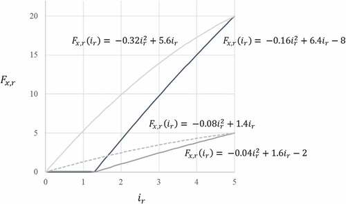
To illustrate the concept, Figure 2 presents examples of the component return function based on two quality levels, {poor, good}, where the horizontal axis represents the incentive given and the vertical axis the components returned. Each of the two functions behaves differently as the incentive provided to the return market r increases. For example, the function indicates a non-zero number of returns when poor condition at point (the leftmost graph), and zero returns when good condition at the same incentive level (the centre graph). Figure 2 presents the sum of the returns for both quality levels, therefore the maximum total number of components (in all possible quality conditions) from the return source .

Figure 2. Example of the component return function.

The model considers different return scenarios to characterise the stochastic nature of returns. Let represent the set of return levels. Each level relates to a percentage of the maximum units to be returned. The assumption of a maximum level of returns is congruent with previous research (Das and Dutta 2016) as this considers estimates about previously sold units (what is already in the market) and expected time to EoL and EoU, in combination with a top value for the incentive offered to returners. Let represent the percentage of maximal returns received under return level z from return source r. Therefore, the expected number of units in condition to be received from the return source when the incentive to that source is and under return level z equals . To illustrate this concept, consider there are two return levels, {high, low} and the values of and are 100% and 60%, respectively. The left graph of Figure 3 presents the components returned (vertical axis) without considering the return level, while the graph to the right presents the units returned considering the two values of parameter .

Figure 3. Example of the percentage of maximum demand parameter.

3.3 New components suppliers

The manufacturer can purchase the new component from multiple suppliers. Suppliers are independent of each other, and each has an objective to maximise the reserved capacity and the units purchased by the remanufacturing organisation. Let S represent the set of possible suppliers. The manufacturer determines the capacity to be reserved from each supplier and let be the reserved capacity from the supplier . The model assumes there is no minimum or maximum reserved capacity and if , the supplier is not part of the supply system. As previously stated, the quantity returned by each source is random, and therefore the number of units to be purchased from the suppliers depends on the returns. Furthermore, there is the possibility of supplier disruption during a cycle due to internal and external factors (lack of raw materials, worker strikes, natural disasters, etc.). In such cases, the supplier cannot deliver any number of components. The model assumes return quantities and supplier failures are known at the start of the cycle, therefore the suppliers that are operational (not in a disruption state) can produce to meet the required demand. This assumption is similar to Meena and Sarmah (2016), and Esmaeili-Najafabadi et al. (2019) which suppose real-time information flows and strong collaborative efforts with suppliers that allow the manufacturer to determine the status of its supplier orders and return sources in the early stages of a cycle.

3.4 Scenarios and units received from all flows

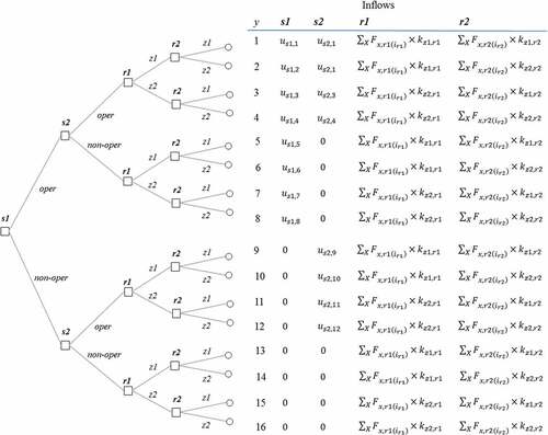
As described in the previous sections, the model considers two random elements: the possibility that suppliers do not deliver and the return quantity per return source. Thus, the different scenarios represent the variability of what suppliers deliver and what returners actually return. Let represent the total number of suppliers, return sources, quality levels, and return quantity levels, respectively. The problem is modelled as a decision tree where there are possible combinations that characterise which suppliers deliver/do not deliver and there are combinations that describe the combined return quantity levels for all the sources (assuming all suppliers have > 0). Therefore, there are states of nature, and each state of nature can be interpreted as a scenario in the stochastic programming context. Let Y be the set of possible states of nature.

Let be the number of units purchased from supplier s under a state of nature y with the constrain that cannot be larger than In other words, the units purchased from a supplier cannot exceed the reserved capacity from that supplier. Figure 4 presents the structure of an environment where , and are all equal to 2 and (only one quality level). On the right of the figure presents the inflows under each of the 16 possible states of nature. In the first four states of nature, both suppliers are operational and therefore deliver, while in the remaining 12 at least one of the suppliers is not operational, and therefore the manufacturer receives 0 units from that source.

Figure 4. Examples of component inflows for all the possible states of nature.

The model assumes that regardless of the incentive level, the component requirement d will always at least equal to the sum of maximal returns from all return sources, under all possible states of nature: . This assumes that the quantity returned will not meet the demand for a cycle, which is in line with models such as Özkır and Başlıgıl (2012) and Pedram et al. (2017). Let represent the total number of units received from the return sources for a state of nature , let represent the total number of units received from the suppliers, and ] represent the unsatisfied demand for each state of nature y. To assist in understanding the service level implications of the decisions, the percentage of requirements satisfied is tracked; let represent the percent of the requirements satisfied during the state of nature : .

3.5 Probabilities

Each state of nature (scenario) y has a probability . This probability is based on two main elements: the probability of suppliers’ disruption and the probability of return quantity levels from the return sources. To model the first, let be a binary variable equal to 1 if supplier s is operational and delivers (i.e. not in a disrupted condition) during the state of nature y, and 0 if it does not. To model the second, let be the random vector that denotes the return quantity level for source s. Since is a finite discrete set, the combination of has a finite number of possible realisations indexed by y, and let be the return quantity level for each return source in , for a return state of nature y. Let be the probability that supplier s delivers during a cycle and let be the probability of return quantity level z from return source r. The probability of a state of nature is and let . Note that if none of the suppliers in is used (i.e. ), then . The resulting values of are used to calculate expected costs as described in the following section.

3.6 Costs

The model considers the following: costs to acquire and transform components to as new condition, incentives paid to returners, cost to reserve capacity from each supplier, purchasing costs for new components, and the loss costs due to unsatisfied demand. Let be per unit cost to acquire/transform to a new component in condition x from return source r. As mentioned earlier, is the incentive paid per unit sourced from return source r. Let and be the reservation and purchasing cost per component for the supplier . Finally, let be loss cost per component not available to meet the per cycle requirements.

The following presents the costs that are determined per state of nature (scenario). Let ,, and represent the costs related to acquisition/remanufacture, incentives, purchasing and losses for a state of nature :

The respective expected total costs are the summation of each scenario costs by its probability. Let TAC, TIC, TPC, and TLC be the expected acquisition/remanufacturing, incentive, purchasing, and loss costs when all the states of nature are considered: , , and . The total reservation costs are and let . Note that the reservation capacity cost does not depend on the state of nature assuming this cost is based on a fixed contract. The total model costs are and let .

3.7 Proposed model

The proposed model has the objective function to under the following constraints:

(1)

(2)

(3)

(4)

(5)

(6)

Constraint (1) guarantees that the incentive per component does not exceed the maximum. Constraint (2) establishes that the units received from a supplier for a state of nature do not exceed the reserved capacity and are received only when the supplier is operational (not in a disrupted condition). Constraints (3) to (6) guarantee that the incentives, quantity to be acquired from the suppliers, the unsatisfied demand, and the reserved capacity from the suppliers are non-negative. While not an element of the mathematical model, the total expected service level is and let

3.8 Model limitations and applicability

The proposed model is an analysis tool that captures a limited set of key variables a real-world manufacturer would have to consider but is based on certain assumptions, such as supplier disruption information, which may not hold in many industrial settings. However, the model can serve as an initial assessment and decision-making tool for a more comprehensive modelling approach. Obtaining the data and parameters that are fed into the model also presents challenges for its applicability, given it depends on forecasts and random variables. Supplier-related parameters would be derived from supplier scorecards or other delivery reliability measures. Parameters related to the return sources would be based on historical records of returns, with a particular need to model the effect of incentives on returns. Organizations may need to perform ‘experiments’ where incentives are given on a temporary basis to understand their effect on the return levels and therefore be able to develop functions that predict that behaviour. As demonstrated by the sensitivity analysis (Section 5), the supplier portfolio and incentive decisions are highly dependent on the parameters, therefore in applications of this model, it would be important to consider the variability of the data and the resulting parameters. It would be important in applications of the model to use various values of the parameters based on the collected data to evaluate the robustness of the recommendations. While capturing this type of information may be time-consuming and will never be perfect, good approximations could be developed over time that would allow a manufacturer to use the model to have a much better sense of the supplier set to use, the capacity to reserve and the incentives to offer, than a ‘blind’ approach to these decisions.

4. Numerical example

This section presents a numerical example to illustrate the model. It is assumed a mechanical component has a per cycle demand (requirement) of 90 units (i.e. ). Not having this component results in a loss cost of $100 (i.e. ). The example assumes there are two suppliers (i.e., ) that can provide this mechanical component as a new item. Furthermore, it is assumed there are three possible return sources (i.e. ), where the component can be obtained and then remanufactured. The components are returned in two possible quality conditions (i.e., , {good, poor}), therefore there are six incentive functions that model the amount returned by a source (three return sources × two possible conditions). The percentage of components returned by all the return sources is modelled at two levels and has the same value for the percentage parameter (i.e., , {max, mid} and ). Therefore, in half the states of nature, the amount returned by a source would be the maximal amount and in remaining states of nature, it would be half that maximal amount.

Table 2 presents the parameters related to the two suppliers. Note that the supplier is more reliable ( = probability of delivery per cycle; probability of no internal or external disruptions) and more expensive than the supplier for both the reservation cost and the purchase cost per item. Table 3 presents the parameters related to the three return sources. For each of the two possible return conditions {= good and poor}, the table presents the return function (i.e. ), the probability at = max (i.e. ), and the cost to acquire/remanufacture a component (i.e. ). Given there are only two return levels, is the complement of .

Table 2. Suppliers’ information.

Supplier ()
	99%	85%
	$3	$2
	$11	$10.5

Table 3. Returners’ information.

	Return source ()
Good
		50%	30%	70%
		$5	$6	$7
Poor
		60%	80%	40%
		$11	$9	$10

Figure 5 presents the four functions that determine the number of components returned based on the incentive provided. The maximum per component incentive that can be allocated to any of the return sources is $5/unit (). In the application of the functions, all values of where < 0 are replaced by (returns cannot be negative).

Figure 5. Return functions used in the example with .

4.1 Two illustrative cases

Two cases (solutions) are presented to illustrate the mechanics of the model. The first case assumes the amount reserved from the two suppliers is 0, . Therefore, only returned components are used to meet the required units, and . Furthermore, the three return sources receive the following incentives per unit returned: (). Based on these incentives and the maximal return equation, the maximal number of units is determined (for example, ). Therefore, the maximal number of good units to be returned by return sources , and are 15.04, 0 and 20, respectively, while the maximal number of poor units is 4.3, 5.3 and 20, respectively. As an expected value model real numbers are used even when components are integer values.

Table 4 presents a subset of the 64 states of nature that apply to this case. Only 64 states of nature apply in this case as supplier-related states of nature are not relevant (for each supplier the number of states of nature increases by a factor of 2 representing if they deliver or not during a cycle). For each state of nature the table includes the return quantity level for each return source and quality condition, its probability (), the total number of returns (), the number of components missing (), the acquisition/remanufacturing costs (), the incentive costs () and the loss costs (). The complete process calculations for the state of nature 1 are:

Table 4. Calculations per state of nature (partial) for the example under the first case.

		1	2	3	4		61	62	63	64
		max	max	max	max		mid	mid	mid	mid
good		max	max	max	max		mid	mid	mid	mid
		max	max	max	max		mid	mid	mid	mid
		max	max	max	max		mid	mid	mid	mid
poor		max	max	mid	mid	…	max	max	mid	mid
		max	mid	max	mid		max	mid	max	mid
		0.0202	0.0302	0.005	0.0076		0.0134	0.0202	0.0034	0.0050
		64.64	54.64	62	52		45	35	42.32	32.32
		25.36	35.36	28	38		45	55	47.68	57.68
		¤510	410	486	386		379	279	355	255
		283	233	280	230		194	144	191	141
		2,536	3,536	2,800	3,800		4,504	5,504	4,768	5,768

(Given )

For this case, the resulting overall expected measures are , for a . The for this case is 60.49%.

The second case assumes the supplier has a reserved capacity of 30 units (i.e. ), has a reserved capacity of 20 units (i.e. ) and the incentives provided are the same as in the first case. Table 5 presents a subset of the 256 states of nature. Table 4 includes the return quantity level for each return source and quality condition, and the binary variable , which indicates if a supplier is operational and delivers during the state of nature . In state of nature 1 both suppliers deliver, in state of nature 2 only supplier delivers, in state of nature 3 only supplier delivers, and in state of nature 4 none of the suppliers deliver. The table also includes for each state of nature its probability (), the total number of returns (), the number of units purchased from each supplier (), the total number of units purchased from suppliers (), the number of components missing (), the acquisition/remanufacturing costs (), the incentive costs (), the purchasing costs () and the loss costs (). The complete process calculations for the state of nature 1 are:

Table 5. Calculations per state of nature (partial) for the example under the second case.

		1	2	3	4		253	254	255	256
		max	max	max	max		mid	mid	mid	mid
good		max	max	max	max		mid	mid	mid	mid
		max	max	max	max		mid	mid	mid	mid
		max	max	max	max		mid	mid	mid	mid
poor		max	max	max	max	…	mid	mid	mid	mid
		max	max	max	max		mid	mid	mid	mid
		1	1	0	0		1	1	0	0
		1	0	1	0		1	0	1	0
		0.0163	0.0029	8.6E-4	1.5E-4		0.0041	7.2E-4	2.1E-4	3.8E-5
		64.64	64.64	64.64	64.64		32.32	32.32	32.32	32.32
		5.36	30	0	0		30	30	0	0
		20	0	20	0		20	0	20	0
		25.36	25.36	20	0		50	30	20	0
		0	0	5.36	25.36		7.68	27.68	37.68	57.68
		510	510	510	510		255	255	255	255
		283	283	283	283		141	141	141	141
		269	330	210	0		540	330	210	0
		0	0	536	2,536		768	2,768	3,768	5,768

;

(as shown in the previous case).

Note that determining the units purchased is based on a simple logic: purchase from the suppliers that can deliver in that state of nature, selecting by lowest up to max (reserved capacity, needed units) until either no units is needed or all reserved capacities have been used.

(Shown in the previous case).

(Shown in the previous case).

For the second case, the resulting overall expected measures are . The costs to reserve the capacity are , for . The for this case is 97.14%. Clearly, reserving capacity from the suppliers and then purchasing new units results in a lower cost and a higher service level. The question is, what is the best solution?

4.2 Best solution found

Determining an optimal solution to the proposed model is challenging due to its non-linear nature. This research focused on developing a model and decision-making framework, and to find a good solution we used full enumeration of a reduced search space. In the reduced search space, incentive values are considered in steps of 0.5: 0, $0.5, $1, …, $4.5, $5 ($5 is the maximum incentive in all cases); while the number of units to be reserved from each supplier is considered in steps of 10 units; 0, 10, 20, up to 90 (90 is the maximum demand). Thus, the search space is made by 133,100 combinations of incentive and reserve unit values. The total costs are determined for all the 133,100 combinations to establish the best solution to a problem instance.

Using the full enumeration approach for this reduced search space, the best solution found has a value of 1,204 and of 99.58%. This solution is based on the following decisions: . Therefore, the solutions presented previously are ‘far’ from the best possible. It is worth noting that using the reduced search space approach would be in line with many practical settings where the amounts that can be ordered from suppliers would be based on batch size and where incentives would be rounded to a ‘sensible’ value. Furthermore, a higher precision level can be obtained by increasing the granularity of the incentive steps and unit amounts (due to higher CPU capabilities). This approach to finding a solution does have limitations as the number of suppliers or incentive granularity increases, requiring exponentially growing computational times, which would limit the model’s applicability. Extensions to this research may include the development of a MILP where the non-linear functions are linearised using the piecewise linearisation technique (Geißler et al. 2012).

5. Sensitivity analysis

This section presents a sensitivity analysis of the previous example. The objective of this analysis is to describe how different parameters influence the decision variables. All the solutions presented are based on the best solution found using full enumeration of the reduced search space. Sensitivity analysis is conducted in relation to four factors: supplier reliability (ability to deliver considering internal and external disruptions), supplier cost structure, loss cost, and the percentage of maximal returns.

5.1 Supplier reliability

The base example considers the following two supplier reliability values: , thus there is a significant difference between the reliability of the two suppliers. The first experiment evaluates the effect of changes on the reliability of on decisions and costs. Table 6 presents the resulting decisions and costs as the reliability of is modified to 0.99, 0.95, 0.9, 0.8, 0.75, and 0.7 (the baseline case is shaded). As the reliability of increases, incentives are reduced slightly at 0.9, and then the reserved quantity increases at from 10 to 20 units. When supplier is as reliable as supplier , supplier becomes the sole source, and the incentives are reduced slightly. On the other hand, as the reliability of decreases, there is a small increase in incentives at , and then at supplier is no longer used, thus becoming a sole sourcing environment. The total reserved capacity () is 60 for all levels up to = 0.7, where the reserved capacity falls to 50. The incentives do not vary considerably, with a maximum range of 1 across the considered values of ( at ; at ).

Table 6. Experiments with at baseline and changes to .

0.99	0.99	0	60	4	2.5	2.5	$1,131	99.5%
	0.95	40	20	4.5	3	3	$1,192	99.6%
	0.90	50	10	4	2.5	3	$1,201	99.5%
	0.85	50	10	4.5	2.5	3	$1,204	99.6%
	0.80	50	10	4.5	2.5	3	$1,207	99.5%
	0.75	50	10	4.5	3	3	$1,210	99.6%
	0.70	50	0	4.5	3	3.5	$1,210	99.5%

The second analysis considers changes to the reliability of both suppliers; and is considered at 0.95, 0.9, 0.85 up to 0.1. Table 7 presents only the results where there is a change to one of the decision variables (for example, there is no row for as the decisions are the same as for ). In these experiments, when both suppliers have a reserved capacity even when supplier is less expensive. This result is different than when (Table 6), where only supplier had a reserved capacity. From this point on, as decreased, the allocation to decreased, while incentives increased. However, it is interesting to note that had a reserved capacity up to . There is no reserved capacity for supplier at or lower. This is a noteworthy difference from the cases where , where became the sole source when reached 0.7. Another interesting effect is how the total reserved capacity decreased as decreased; from 70 at to 40 at (with ). This is also noteworthy as the reserved capacity of did not increase to replace that ‘taken’ from and only an increase in incentives is used to counter the effect. In this case, the incentive for is at the maximum level for all tested values of , while it varies by 1 for and . The decreased by almost 1% as the reliability for supplier decreased from 0.95 to 0.3 and different decisions are made.

Table 7. Experiments with = 0.95 and changes to .

0.95	0.95	30	40	5	3	3.5	$1,220	99.5%
	0.90	30	30	5	4	4	$1,242	99.5%
	0.85	40	30	5	3.5	3.5	$1,255	99.4%
	0.80	40	30	5	3.5	4	$1,265	99.5%
	0.65	40	20	5	3.5	4.5	$1,291	99.2%
	0.45	40	10	5	4	4.5	$1,312	98.9%
	0.30	40	0	5	4	4.5	$1,319	98.6%

5.2 Supplier cost structure

The second factor under consideration is the suppliers’ cost structure. In the base case, the reservation costs are significantly lower than the purchase cost. This assumption is modified and experiments are performed where the reservation and purchase cost per component are fairly equal. Note that the total cost per supplier () does not change.

Low reservation costs:

High reservation costs:

The first set of experiments described in Section 5.1 are repeated under the new cost structure (where is changed from 0.99 to 0.7). Table 8 presents the results with the high reservation cost structure (first three rows), followed by the results from Table 6 (repeated to ease the comparison). At , the new cost structure results (in high reservation costs) in a higher reservation capacity and lower incentives than when the low reservation cost structure is used. This result is counter-intuitive as it would be logical that higher reservation costs would lead to lower reserved capacity. However, this increase in reservation capacity is accompanied by a notable reduction in incentives. As decreased from 0.99 to 0.95, the total reserved capacity in the high-cost structure case decreased from 70 to 50, but then increased to 60 when . The cost structure change also has an effect on the point where supplier is not used; in the low reservation cost structure is no longer used at , while in the high reservation cost structure, is not used at . Overall, incentives are lower with the high reservation structure than at the low structure. Finally, there is no notable change in the based on the different cost structures.

Table 8. Experiments with changes to and high reservation cost structure.

	reservation costs
0.99	high	0.99	0	70	3	1	2	$1,171	99.2%
		0.95	40	10	4	3	3.5	$1,244	99.4%
		0.85	60	0	3.5	2.5	2.5	$1,256	99.4%
	low	0.99	0	60	4	2.5	2.5	$1,131	99.5%
		0.95	40	20	4.5	3	3	$1,192	99.6%
		0.90	50	10	4	2.5	3	$1,201	99.5%
		0.85	50	10	4.5	2.5	3	$1,204	99.6%
		0.80	50	10	4.5	2.5	3	$1,207	99.5%
		0.75	50	10	4.5	3	3	$1,210	99.6%
		0.70	50	0	4.5	3	3.5	$1,210	99.5%

5.3 Loss cost

The third factor under consideration is the loss costs parameter (). This parameter represents the financial burden on the organisation for not having the required number of components on a cycle. The parameter baseline value is $100, and four additional levels are considered: $25, $50, $200 and $400. Table 9 presents the results based on the baseline case: and the low reservation cost structure. Values of lower than $100 result in minor changes to the decisions when compared to . On the other hand, as increased from 100 to 200, there is an increase in all the incentives, but no increase in reserved capacity, while at there is an increase in the reserved capacity (up to 90 which represents the total demand d) and the incentives are decreased from . Therefore, an interesting balancing act exists between incentives and reserved capacity as increases. Also, as expected, as increased, increased, indicating that losses become much more relevant in the total cost structure.

Table 9. Experiments considering changes to .

0.99	0.85	25	40	10	4.5	2.5	3	$1,157	98.6%
		50	50	10	4	2.5	3	$1,180	99.5%
		100	50	10	4.5	2.5	3	$1,204	99.6%
		200	40	20	5	3.5	4	$1,239	99.8%
		400	50	40	4.5	3	3.5	$1,267	99.9%

Two additional cases are analysed to further understand the effect of parameter . Table 10 presents the case where and low reservation cost structure. This case is interesting as it demonstrates the interaction between supplier reliability and . For example, the capacities reserved per supplier are notably different when comparing the first row of Table 10 to the first row of Table 9 (). Furthermore, the at is 96.3%, a relatively low value compared to any of the previous results. However, as increased, the increased to 99.8%, in line with previous results.

Table 10. Experiments considering changes to with = 0.95.

0.95	0.85	25	20	30	4.5	2.5	3.5	$1,170	96.3%
		50	30	20	5	3.5	4	$1,216	98.8%
		100	40	30	5	3.5	3.5	$1,255	99.4%
		200	40	40	5	3.5	4	$1,296	99.7%
		400	40	40	5	3.5	4.5	$1,348	99.8%

Table 11 presents the case where and low reservation cost structure. This case is relevant as it demonstrates the interaction between supplier reliability, , and the use of a supplier. Note that the capacity reserved from the high-reliability supplier () does not change regardless of the value of , demonstrating a robust recommendation regarding that parameter. By contrast, the unreliable supplier () is not part of the supply network () until equals 200. Note that while supplier is unreliable, its reserved capacity increased as increased from 200 to 400, while two of the three incentive decisions stayed the same.

Table 11. Experiments with changes to and .

0.99	0.70	25	50	0	4	2.5	3	$1,163	98.7%
		50	50	0	4.5	3	3	$1,184	99.3%
		100	50	0	4.5	3	3.5	$1,210	99.5%
		200	50	10	4.5	3	3.5	$1,248	99.7%
		400	50	30	5	3	3.5	$1,292	99.8%

5.4 Percentage of maximal returns

The fourth analysed factor is the percentage of maximal returns, . The baseline case assumes the same two levels for all three return sources and the two conditions: {max, mid} and . Therefore, either all or half the forecasted returns (based on the incentive equation) are received depending on the state of nature, for an average of 75% of the maximal returns (ave [50%, 100%] = 75%). This section evaluates changes to the percentage that models the mid-level, . The value of is examined at 20%, 35%, 50% (the baseline), 65% and 85% for all return sources . This represents changes to the behaviour of the return sources, where the 20% would represent cases with high variability in the quantity returned (in some states of nature is 20%, in others is 100% of the maximal forecasted return quantity) and the average quantity is smaller than the baseline (ave [20%, 100%] = 60%). The 80% level represents the case where there is a small variability in the quantity returned (in some states of nature is 80%, in others is 100% of the maximal forecasted return quantity) and the amount is larger than the baseline (ave [80%, 100%] = 90%). Given the demonstrated effect of the loss cost in the decisions, the experiments are conducted at the baseline case of =$100, and when = $400.

The results under the low reservation cost structure are presented in Table 12. When comparing the decisions to the baseline case at , a lower results in lower incentives and a higher total reserved capacity (), while the opposite occurs when increases. For the range of values of 20% to 80%, the total reserved capacity changed from 80 to 40, while incentives increased by an average of 0.5. A similar effect is observed at where the total reserved capacity decreased, and the incentives increased as increased. This case is notable as it represents the first set of experimental combinations (when = 20% and 35%) where the total reserved capacity exceeds the demand (). When and for the range of values of 20% to 80%, the total reserved capacity changed from 120 to 50, while incentives increased by an average of 0.833.

Table 12. Results of the experiments with changes to under the low reservation cost structure.

0.99	0.85	100	20%	60	20	4	2.5	3	$1,254	99.5%
			35%	60	10	4	2.5	3	$1,230	99.6%
			50%	50	10	4.5	2.5	3	$1,204	99.6%
			65%	40	10	4.5	3	3	$1,180	99.6%
			80%	30	10	4.5	3	3.5	$1,157	99.7%
		400	20%	70	50	4	2.5	3	$1,339	99.9%
			35%	60	40	4.5	2.5	3.5	$1,304	99.9%
			50%	50	40	4.5	3	3.5	$1,267	99.9%
			65%	40	30	4.5	3.5	3.5	$1,229	99.9%
			80%	30	20	5	3.5	3.5	$1,194	99.9%

Table 13 presents the results under the high reservation cost structure. When and comparing the results to the low reservation cost structure, both the incentives and the total reserved capacities are smaller. Furthermore, under all levels of only is used. At , the total reserved capacities are significantly lower than at . For example, the total reserved capacity ranged from to 70 at and ranged from 50 to 20 at . On the other hand, incentives are higher at , almost to their maximum value for all three return sources at .

Table 13. Results of the experiments with changes to under the baseline cost structure.

0.99	0.85	100	20%	70	0	3.5	2	2.5	$1,321	99.0%
			35%	70	0	3	1.5	2.5	$1,291	99.3%
			50%	60	0	3.5	2.5	2.5	$1,256	99.4%
			65%	50	0	4	2	3	$1,218	99.4%
			80%	40	0	4.5	2.5	3	$1,177	99.6%
		400	20%	60	10	4.5	3.5	4	$1,507	99.6%
			35%	50	10	5	3.5	4	$1,441	99.7%
			50%	40	10	5	4	4	$1,378	99.8%
			65%	30	10	5	3.5	4.5	$1,318	99.8%
			80%	20	0	5	4.5	4.5	$1,254	99.8%

5.5 Summary of results

The sensitivity analysis demonstrates that decisions regarding the set of suppliers to use, the amount of capacity to reserve, and the incentive to offer the returners (Introduction Section, questions 1 to 3) vary significantly depending on the values of the considered reliability and loss cost parameters. As the reliability of one of the suppliers decreases (higher probability of disruption to the supplier), incentives are increased to reduce this effect and less capacity is reserved for the less reliable supplier. However, some capacity is acquired even when the supplier is highly unreliable. When both suppliers have a relatively high probability of disruption, the total amount of reserved capacity either stays the same or increases, and the incentives increase. The cost structure of the suppliers is also highly intertwined with the decisions, and the resulting best decisions when the reservation costs increased included increases in the reserved capacity and a reduction in incentives.

Furthermore, the loss cost and its interaction with the reliability of suppliers significantly influences the decisions (Introduction Section, questions 4 and 5): higher loss costs result in higher reservation capacities and incentives, although the particular combination depends on the reliability of the suppliers. It is interesting to note that total costs are higher when the system has as options two ‘middle of the road’ suppliers (Table 10), than when it has as options one highly reliable supplier and one unreliable supplier (Table 11). This is attributed to the decision not to use the unreliable supplier when the loss costs are low and only reserve capacity from this supplier as the loss costs increase significantly.

Finally, the average and range of quantities returned have a notable impact on the decisions (Introduction Section, question 6), thus from the managerial perspective understanding the behaviour of the return sources in relation to incentives and to different states of nature may be the most important data collection process related to implementing a model such as the one described here. A combination of high loss costs, low reservation costs, and scenarios with low return quantities result in total reserved capacities above the total demand required and on low incentives. This means that to minimise costs, extra capacity is being reserved to protect against the lack of returns. However, when the reservation costs are high, both incentives and the total reserved capacity decrease. Under the parameter combinations where the return quantities and the reservation costs are high, incentives are increased almost to their maximum while there is almost no reserved capacity from the suppliers.

6. Conclusions and future research

Uncertainty in both forward and reverse elements of CLSC networks create complexity and pose challenges to its management and optimisation. The sources of uncertainty are numerous. On the forward side, internal and external disruptions can prevent new components from arriving to the production system. On the reverse side, there is uncertainty related to the quality and the quantity of the returns. Quantifying and understating uncertainties is highly relevant as it has a significant impact on the costs and benefits of remanufacturing. Thus, decision-making must focus on controlling elements that regulate the supply chain network.

This paper presents a model that supports the control of several relevant elements of a remanufacturing network. On the forward side, it determines the suppliers of new components to be used in the system, the capacity to be contracted from each selected supplier, and operationally the amount to be ordered per supplier during each scenario. On the reverse side, the model determines the incentive to each return source considering a quantity function per quality condition. The model captures uncertainty by considering multiple scenarios related to supplier deliveries and the quantities of returned items that represent all the combinations of variable elements.

The study presents an example to illustrate the model and conducts a sensitivity analysis considering four factors: a) the suppliers’ ability to deliver considering internal and external disruptions; b) the supplier cost structure which relates to the reservation and purchase costs, c) the loss cost which can be significant in the scenarios with low returns or where suppliers fail to deliver, and d) the percentage of maximal returns which determines the amount returned under a portion of the scenarios. The results indicate the recommended decision is sensitive to changes in these factors; different combinations of the suppliers’ contracted capacity and the incentives to provide each return source resulted in the best outcome. For example, there were experimental conditions where a single supplier was used with a contracted capacity that was a small fraction of the total demand, and other conditions where both suppliers were used and the total contracted capacity exceeded the total demand. Furthermore, there were cases where incentives were used at nearly the maximum possible levels and other cases where incentives were ‘minimally’ used.

The model has several limitations including the fact that it only captures a subset of the characteristics of CLSC networks. For example, factors such as time, degradation, and obsolescence are not considered. Furthermore, obtaining the parameters needed to run the model may be hard to determine (e.g. the function that relates incentives to return quantities per quality level). Another limitation of this research is the use of a full enumeration approach to generate a good solution. This approach requires significant computational time as the problem size increases (i.e. more suppliers, more return sources, and more return conditions). MILP Models based on piecewise linearisation could be developed, which in combination with solvers such as Gurobi and CPLEX would enable tackling larger problems. Solution approaches such as the one proposed in Glock (2011) could be modified to address the problem described in this paper for large-sized cases.

The relevance of CLSCs, reverse logistics, and remanufacturing continues to grow, thus the need for much additional research. Future areas of recommended research include models that study incentives that take into consideration the condition of the returns based on the duration of use and the use of incentives only in particular scenarios. Revisions of the model that allow for larger problems would also be a useful extension. Other directions for future research include considerations related to the location and transportation of the new and used components, as well as the uncertainty of the demand.

Disclosure statement

No potential conflict of interest was reported by the author(s).

Additional information

Notes on contributors

Alex J. Ruiz-Torres

Dr. Alex Ruiz-Torres is a full time faculty member at the Facultad de Administracion de Empresas at the University of Puerto Rico, Rio Piedras Campus. He received his Bachelor, Masters, and Ph.D. degrees in Industrial Engineering from Georgia Tech, Stanford, and Penn State respectively. Past awards include being the Fulbright - Aalto University Distinguished Chair (Helsinki, Finland), a Prometeo fellowship from SENESCYT (Ecuador), and a Fulbright Scholar award at Escuela Politecnica Nacional (Quito, Ecuador). He has also been awarded two NASA faculty fellowships at the Kennedy Space Center and a NASA Small Business Technology Transfer grant. He has over sixty journal publications with research interests including multi-criteria production planning models and closed loop robust supply chain systems.

Farzad Mahmoodi

Farzad Mahmoodi is Joel Goldschein ’57 Endowed Chair Professor in Supply Chain Management and the Director of Clarkson University’s nationally ranked Global Supply Chain Management Program. He has published about 100 articles in leading journals. Dr. Mahmoodi has been the recipient of numerous awards, including multiple Professor of the Year Award (MBA Program), Lifetime Achievement in Research and Scholarship Award, the Commendable Leadership Award, the Distinguished Teaching Award, the Clarkson University Student Association Teaching Award and the John W. Graham, Jr. Faculty Research Award. He serves on the editorial boards of the International Journal of Industrial Engineering and the International Journal of Integrated Supply Management. His research interests focus on design and control of manufacturing and logistics systems.

Shunichi Ohmori

Shunichi Ohmori (PhD) is an associate professor at Department of Industrial & System Engineering, Waseda University in Japan, and a researcher at Institute of Global Production & Logistics at Waseda University, and a researcher at Data Science Institute at Waseda University. He received the master and Ph.D degrees in engineering from Waseda University. His research interest lies in operations research and supply chain management.

Arbia Hlali

Arbia Hlali is a doctor of economics science from the Faculty of Economics and Management of Sfax, University of Sfax, Tunisia. Presently working as assistant professor at the Mediterranean Institute of Nabeul. She holds a master of transport and logistics sciences from the higher Institute of industrial management of Sfax, Tunisia. She has worked as assistant professor in different universities in Tunisia. Her research interest includes logistics and supply chain, maritime transport, port management, transport economics, sustainability development, entrepreneurship, business economics, and blockchain

References

- Abdolazimi, O., M. S. Esfandarani, M. Salehi, and D. Shishebori. 2020. “Robust Design of a multi-objective closed-loop Supply Chain by Integrating on-time Delivery, Cost, and Environmental Aspects, Case Study of a Tire Factory.” Journal of Cleaner Production 264: 121566. doi:10.1016/j.jclepro.2020.121566.
- Agrawal, S., R. K. Singh, and Q. Murtaza. 2015. “A Literature Review and Perspectives in Reverse Logistics.” Resources, Conservation and Recycling 97: 76–92. doi:10.1016/j.resconrec.2015.02.009.
- Battini, D., M. Bogataj, and A. Choudhary. 2017. “Closed Loop Supply Chain (CLSC): Economics, Modelling, Management and Control.” International Journal of Production Economics 183 (2): 319–321. doi:10.1016/j.ijpe.2016.11.020.
- Berger, P. D., A. Gerstenfeld, and A. Z. Zeng. 2004. “How Many Suppliers are Best? A Decision Making Approach.” Omega 32 (1): 9–15. doi:10.1016/j.omega.2003.09.001.
- Bhattacharya, R., A. Kaur, and R. K. Amit. 2018. “Price Optimization of multi-stage Remanufacturing in a Closed Loop Supply Chain.” Journal of Cleaner Production 186: 943–962. doi:10.1016/j.jclepro.2018.02.222.
- Braz, A. C., A. M. De Mello, L. A. de Vasconcelos Gomes, and P. T. de Souza Nascimento. 2018. “The Bullwhip Effect in closed-loop Supply Chains: A Systematic Literature Review.” Journal of Cleaner Production 202: 376–389. doi:10.1016/j.jclepro.2018.08.042.
- Chai, J., J. N. Liu, and E. W. Ngai. 2013. “Application of decision-making Techniques in Supplier Selection: A Systematic Review of Literature.” Expert Systems with Applications 40 (10): 3872–3885. doi:10.1016/j.eswa.2012.12.040.
- Coenen, J., R. E. Van der Heijden, and A. C. van Riel. 2018. “Understanding Approaches to Complexity and Uncertainty in closed-loop Supply Chain Management: Past Findings and Future Directions.” Journal of Cleaner Production 201: 1–13. doi:10.1016/j.jclepro.2018.07.216.
- Das, D., and P. Dutta. 2016. “Performance Analysis of a closed-loop Supply Chain with incentive-dependent Demand and Return.” The International Journal of Advanced Manufacturing Technology 86 (1–4): 621–639. doi:10.1007/s0017.
- De Giovanni, P., P. V. Reddy, and G. Zaccour. 2016. “Incentive Strategies for an Optimal Recovery Program in a closed-loop Supply Chain.” European Journal of Operational Research 249 (2): 605–617. doi:10.1016/j.ejor.2015.09.021.
- De Giovanni, P., and G. Zaccour. 2019. “A Selective Survey of game-theoretic Models of closed-loop Supply Chains.” 4OR- A Quarterly Journal of Operations Research 17 (1): 1–44. 10.1007/s1028
- Esmaeili-Najafabadi, E., M. S. F. Nezhad, H. Pourmohammadi, M. Honarvar, and M. A. Vahdatzad. 2019. “A Joint Supplier Selection and Order Allocation Model with Disruption Risks in Centralized Supply Chain.” Computers & Industrial Engineering 127: 734–748. doi:10.1016/j.cie.2018.11.017.
- Fathollahi-Fard, A. M., M. A. Dulebenets, M. Hajiaghaei–Keshteli, R. Tavakkoli-Moghaddam, M. Safaeian, and H. Mirzahosseinian. 2021. “Two Hybrid meta-heuristic Algorithms for a dual-channel closed-loop Supply Chain Network Design Problem in the Tire Industry under Uncertainty.” Advanced Engineering Informatics 50: 101418. doi:10.1016/j.aei.2021.101418.
- Geißler, B., A. Martin, A. Morsi, and L. Schewe. 2012. “Using Piecewise Linear Functions for Solving MINLPs.” In Mixed Integer Nonlinear Programming, edited by Leyffer Sven and Lee Jon, 287–314. New York, NY: Springer. doi:10.1007/978-1-4614-1927-3_10.
- Giri, B. C., and S. Sharma. 2016. “Optimal Production Policy for a closed-loop Hybrid System with Uncertain Demand and Return under Supply Disruption.” Journal of Cleaner Production 112: 2015–2028. doi:10.1016/j.jclepro.2015.06.147.
- Glock, C. H. 2011. “A multiple-vendor single-buyer Integrated Inventory Model with A Variable Number of Vendors.” Computers & Industrial Engineering 60 (1): 173–182. doi:10.1016/j.cie.2010.11.001.
- Govindan, K., H. Mina, A. Esmaeili, and S. M. Gholami-Zanjani. 2020. “An Integrated Hybrid Approach for Circular Supplier Selection and Closed Loop Supply Chain Network Design under Uncertainty.” Journal of Cleaner Production 242: 118317. doi:10.1016/j.jclepro.2019.118317.
- Govindan, K., and H. Soleimani. 2017. “A Review of Reverse Logistics and closed-loop Supply Chains: A Journal of Cleaner Production Focus.” Journal of Cleaner Production 142: 371–384. doi:10.1016/j.jclepro.2016.03.126.
- Govindan, K., H. Soleimani, and D. Kannan. 2015. “Reverse Logistics and closed-loop Supply Chain: A Comprehensive Review to Explore the Future.” European Journal of Operational Research 240 (3): 603–626. doi:10.1016/j.ejor.2014.07.012.
- Guide, V. D. R., Jr, R. H. Teunter, and L. N. Van Wassenhove. 2003. “Matching Demand and Supply to Maximize Profits from Remanufacturing.” Manufacturing & Service Operations Management 5 (4): 303–316. doi:10.1287/msom.5.4.303.24883.
- He, Y. 2015. “Acquisition Pricing and Remanufacturing Decisions in a closed-loop Supply Chain.” International Journal of Production Economics 163: 48–60. doi:10.1016/j.ijpe.2015.02.002.
- Hosoda, T., and S. M. Disney. 2018. “A Unified Theory of the Dynamics of closed-loop Supply Chains.” European Journal of Operational Research 269 (1): 313–326. doi:10.1016/j.ejor.2017.07.020.
- Hosseini-Motlagh, S. M., M. Nouri-Harzvili, M. Johari, and B. R. Sarker. 2020. “Coordinating Economic Incentives, Customer Service and Pricing Decisions in a Competitive closed-loop Supply Chain.” Journal of Cleaner Production 255: 120241. doi:10.1016/j.jclepro.2020.120241.
- Hosseini, S., N. Morshedlou, D. Ivanov, M. D. Sarder, K. Barker, and A. Al Khaled. 2019. “Resilient Supplier Selection and Optimal Order Allocation under Disruption Risks.” International Journal of Production Economics 213: 124–137. doi:10.1016/j.ijpe.2019.03.018.
- Jurburg, D., and M. Tanco. 2017. “Study of the Operational Factors Affecting Productivity in SMEs.” Memoria Investigaciones en Ingenieria 15: 7–23.
- Keyvanshokooh, E., S. M. Ryan, and E. Kabir. 2016. “Hybrid Robust and Stochastic Optimization for closed-loop Supply Chain Network Design Using Accelerated Benders Decomposition.” European Journal of Operational Research 249 (1): 76–92. doi:10.1016/j.ejor.2015.08.028.
- Khatami, M., M. Mahootchi, and R. Z. Farahani. 2015. “Benders’ Decomposition for Concurrent Redesign of Forward and closed-loop Supply Chain Network with Demand and Return Uncertainties.” Transportation Research Part E: Logistics and Transportation Review 79: 1–21. doi:10.1016/j.tre.2015.03.003.
- Liao, H., and L. Li. 2021. “Environmental Sustainability EOQ Model for closed-loop Supply Chain under Market Uncertainty: A Case Study of Printer Remanufacturing.” Computers & Industrial Engineering 151: 106525. doi:10.1016/j.cie.2020.106525.
- Liu, L., Z. Wang, L. Xu, X. Hong, and K. Govindan. 2017. “Collection Effort and Reverse Channel Choices in a closed-loop Supply Chain.” Journal of Cleaner Production 144: 492–500. doi:10.1016/j.jclepro.2016.12.126.
- Lücker, F., R. W. Seifert, and I. Biçer. 2019. “Roles of Inventory and Reserve Capacity in Mitigating Supply Chain Disruption Risk.” European Journal of Operational Research 57 (4): 1238–1249. doi:10.1080/00207543.2018.1504173.
- Mahapatra, M. S., P. C. Pradhan, and J. K. Jha. 2021. “Sourcing Decisions with Order Allocation under Supply Disruption Risk considering Quantitative and Qualitative Criteria.” Operational Research- An International Journal 21: 1–43.
- Masoudipour, E., H. Amirian, and R. Sahraeian. 2017. “A Novel closed-loop Supply Chain Based on the Quality of Returned Products.” Journal of Cleaner Production 151: 344–355. doi:10.1016/j.jclepro.2017.03.067.
- Matsumoto, M., and Y. Umeda. 2011. “An Analysis of Remanufacturing Practices in Japan.” Journal of Remanufacturing 1 (1): 2. doi:10.1186/2210-4690-1-2.
- Meena, P. L., and S. P. Sarmah. 2013. “Multiple Sourcing under Supplier Failure Risk and Quantity Discount: A Genetic Algorithm Approach.” Transportation Research Part E: Logistics and Transportation Review 50 (C): 84–97. doi:10.1016/j.tre.2012.10.001.
- Meena, P. L., and S. P. Sarmah. 2016. “Supplier Selection and Demand Allocation under Supply Disruption Risks.” The International Journal of Advanced Manufacturing Technology 83 (1–4): 265–274. doi:10.1007/s00170-015-7520-5.
- Meena, P. L., S. P. Sarmah, and A. Sarkar. 2011. “Sourcing Decisions under Risks of Catastrophic Event Disruptions.” Transportation Research Part E: Logistics and Transportation Review 47 (6): 1058–1074. doi:10.1016/j.tre.2011.03.003.
- Modak, N. M., N. Modak, S. Panda, and S. S. Sana. 2018. “Analyzing Structure of two-echelon closed-loop Supply Chain for Pricing, Quality and Recycling Management.” Journal of Cleaner Production 171: 512–528. doi:10.1016/j.jclepro.2017.10.033.
- Mondal, A., and S. K. Roy. 2021. “Multi-objective Sustainable Opened- and closed-loop Supply Chain under Mixed Uncertainty during COVID-19 Pandemic Situation.” Computers & Industrial Engineering 159: 107453. doi:10.1016/j.cie.2021.107453.
- OECD Green Growth Studies, (2015). Creating Incentives for Greener Products: A Policy Manual for Eastern Partnership Countries. 10.1787/9789264244542-en
- Özkır, V., and H. Başlıgıl. 2012. “Modelling product-recovery Processes in closed-loop supply-chain Network Design.” International Journal of Production Research 50 (8): 2218–2233. doi:10.1080/00207543.2011.575092.
- Pedram, A., N. B. Yusoff, O. E. Udoncy, A. B. Mahat, P. Pedram, and A. Babalola. 2017. “Integrated Forward and Reverse Supply Chain: A Tire Case Study.” Waste Management 60: 460–470. doi:10.1016/j.wasman.2016.06.029.
- Peng, H., N. Shen, H. Liao, H. Xue, and Q. Wang. 2020. “Uncertainty Factors, Methods, and Solutions of closed-loop Supply chain—A Review for Current Situation and Future Prospects.” Journal of Cleaner Production 254: 120032. doi:10.1016/j.jclepro.2020.120032.
- Ponte, B., M. M. Naim, and A. A. Syntetos. 2019. “The Effect of Returns Volume Uncertainty on the Dynamic Performance of closed-loop Supply Chains.” Journal of Remanufacturing 10 (1): 1–14. doi:10.1007/s13243-019-00070-x.
- Rizova, M. I., T. C. Wong, and W. Ijomah. 2020. “A Systematic Review of decision-making in Remanufacturing.” Computers & Industrial Engineering 147: 106681.
- Ruiz-Torres, A. J., and F. Mahmoodi. 2006. “A Supplier Allocation Model considering Delivery Failure, Maintenance and Supplier Cycle Costs.” International Journal of Production Economics 103 (2): 755–766. doi:10.1016/j.ijpe.2005.09.008.
- Ruiz-Torres, A. J., F. Mahmoodi, and S. Ohmori. 2019. “Joint Determination of Supplier Capacity and Returner Incentives in a closed-loop Supply Chain.” Journal of Cleaner Production 215: 1351–1361. doi:10.1016/j.jclepro.2019.01.146.
- Ruiz-Torres, A. J., F. Mahmoodi, and A. Z. Zeng. 2013. “Supplier Selection Model with Contingency Planning for Supplier Failures.” Computers & Industrial Engineering 66 (2): 374–382. doi:10.1016/j.cie.2013.06.021.
- Sarkar, A., and P. K. J. Mohapatra. 2009. “Determining the Optimal Size of Supply Base with the Consideration of Risks of Supply Disruptions.” International Journal of Production Economics 119 (1): 122–135. doi:10.1016/j.ijpe.2008.12.019.
- Savaskan, R. C., S. Bhattacharya, and L. N. Van Wassenhove. 2004. “Closed-loop Supply Chain Models with Product Remanufacturing.” Management Science 50 (2): 239–252. doi:10.1287/mnsc.1030.0186.
- Sawik, T. 2013. “Selection of Resilient Supply Portfolio under Disruption Risks.” Omega 41 (2): 259–269. doi:10.1016/j.omega.2012.05.003.
- Sawik, T. 2018. “Selection of a Dynamic Supply Portfolio under Delay and Disruption Risks.” International Journal of Production Research 56 (1–2): 760–782. doi:10.1080/00207543.2017.1401238.
- Schramm, V. B., L. P. B. Cabral, and F. Schramm. 2020. “Approaches for Supporting Sustainable Supplier selection-A Literature Review.” Journal of Cleaner Production 273: 123089. doi:10.1016/j.jclepro.2020.123089.
- Snyder, L. V., Z. Atan, P. Peng, Y. Rong, A. J. Schmitt, and B. Sinsoysal. 2016. “OR/MS Models for Supply Chain Disruptions: A Review.” IIE Transactions 48 (2): 89–109. doi:10.1080/0740817x.2015.1067735.
- Stević, Ž., D. Pamučar, A. Puška, and P. Chatterjee. 2020. “Sustainable Supplier Selection in Healthcare Industries Using a New MCDM Method: Measurement of Alternatives and Ranking according to COmpromise Solution (MARCOS).” Computers & Industrial Engineering 140: 106231. doi:10.1016/j.cie.2019.106231.
- Sureeyatanapas, P., K. Sriwattananusart, T. Niyamosoth, W. Sessomboon, and S. Arunyanart. 2018. “Supplier Selection Towards Uncertain and Unavailable Information: An Extension of TOPSIS Method.” Operations Research Perspectives 5: 69–79. doi:10.1016/j.orp.2018.01.005.
- Taleizadeh, A. A., F. Haghighi, and S. T. A. Niaki. 2019. “Modeling and Solving a Sustainable Closed Loop Supply Chain Problem with Pricing Decisions and Discounts on Returned Products.” Journal of Cleaner Production 207: 163–181. doi:10.1016/j.jclepro.2018.09.198.
- Torabi, S. A., M. Baghersad, and S. A. Mansouri. 2015. “Resilient Supplier Selection and Order Allocation under Operational and Disruption Risks.” Transportation Research Part E: Logistics and Transportation Review 79: 22–48. doi:10.1016/j.tre.2015.03.005.
- Weber, C. A., J. R. Current, and W. C. Benton. 1991. “Vendor Selection Criteria and Methods.” European Journal of Operational Research 50 (1): 2–18. doi:10.1016/0377-2217(91)90033-R.
- Wu, G. H., C. K. Chang, and L. M. Hsu. 2018. “Comparisons of Interactive Fuzzy Programming Approaches for Closed-loop Supply Chain Network Design under Uncertainty.” Computers & Industrial Engineering 68. doi:10.1016/j.cie.2018.09.022.
- Yolmeh, A., and U. Saif. 2021. “Closed-loop Supply Chain Network Design Integrated with Assembly and Disassembly Line Balancing under Uncertainty: An Enhanced Decomposition Approach.” International Journal of Production Research 59 (9): 2690–2707. doi:10.1080/00207543.2020.1736723.
- Zeballos, L. J., C. A. Méndez, and A. P. Barbosa-Povoa. 2016. “Design and Planning of closed-loop Supply Chains: A risk-averse Multistage Stochastic Approach.” Industrial & Engineering Chemistry Research 55 (21): 6236–6249. doi:10.1021/acs.iecr.5b03647.
- Zeballos, L. J., C. A. Méndez, and A. P. Barbosa-Povoa. 2018. “Integrating Decisions of Product and closed-loop Supply Chain Design under Uncertain Return Flows.” Computers & Chemical Engineering 112: 211–238. doi:10.1016/j.compchemeng.2018.02.011.