Characterization of an airflow network model by sensitivity analysis: parameter screening, fixing, prioritizing and mapping

Abstract

Due to the over-parameterized models in detailed thermal simulation programs, modellers undertaking validation or calibration studies, where the model output is compared against field measurements, face difficulties in determining those parameters which are primarily responsible for observed differences. Where sensitivity studies are undertaken, the Morris method is commonly applied to identify the most influential parameters. They are often accompanied by uncertainty analysis using Monte Carlo simulations to generate confidence bounds around the predictions. This paper sets out a more rigorous approach to sensitivity analysis (SA) based on a global SA method with three stages: factor screening, factor prioritizing and fixing, and factor mapping. The method is applied to a detailed empirical validation data set obtained within IEA ECB Annex 58, with the focus of the study on the airflow network, a simulation program sub-model which is subject to large uncertainties in its inputs.

Keywords:

• global sensitivity analysis
• airflow networks
• calibration

1. Introduction

Current detailed building energy simulation (BES) tools are capable of representing the main phenomena determining the thermal and energy performance of buildings. However, this achievement in terms of accuracy and fidelity in representing reality entails a high level of complexity of building energy models. In particular, BES models have complicated structures consisting of many in-built sub-models that attempt to represent the physical reality and large numbers of input parameters. Modellers undertaking validation studies find it difficult to identify which parameters are responsible for observed differences between measurements and predictions; those undertaking calibration studies find it difficult to determine which parameters should be adjusted to improve the correspondence between measurements and predictions. Additionally, all the modelling process is affected by uncertainties which, because of the interactions linking the various model inputs, unpredictably propagate through the computer code, resulting in uncertainty in the model predictions.

To build accurate models and to reduce these modelling uncertainties, it is necessary to utilize a detailed building specification. In practice, many model inputs are often not available. Thus although BES tools can be used to predict the detailed spatial and temporal variations in energy and indoor environmental performance, it is difficult to judge the predictive accuracy because of these modelling uncertainties. Ideally, model output uncertainty would routinely be quantified to allow the robustness and reliability of model predictions to be assessed. However in practice, this is seldom the case because of the lack of support to allow users to take into account uncertainties in predictions. The only attempt known to the authors to embed uncertainty analysis (UA) in BES programs is by Macdonald and Strachan (2001) based on the dynamic simulation tool ESP-r (Clarke 2001).

There have been recent attempts to develop methods to tackle these issues and at the same time to better understand and characterize modelling uncertainty propagation within BES tools. In particular, sensitivity analysis (SA) has been increasingly applied in a stand-alone fashion or as a step in more structured procedures, in order to investigate how model parameter uncertainties influence model behaviour and to address the following issues:

• identifying the most influential variables,

• quantifying output uncertainty,

• understanding the relations between inputs, and inputs and outputs,

• supporting decision-making,

• solving identifiability problems.

An extensive review of SA techniques applied to BES can be found in Tian (2013), while a more general treatment focusing on the different problems that different SA methods can solve is in Saltelli et al. (2002).

SA is usually applied by itself to quantify the uncertainty in the model output produced by uncertainties in the model parameters and to understand which are the most influential inputs or, more generally, what the relationships are between the model parameters and model outputs. In Corrado and Mechri (2009), the authors apply the Morris method (1991) and Monte Carlo simulation to identify the most influential factors and the overall output uncertainty for a monthly quasi-steady simplified regulatory model describing a residential building in Turin, Italy. A similar approach is adopted in Garcia Sanchez et al. (2014) to investigate a dynamic ESP-r model representing an apartment building in Spain. In this study, the Morris method in its extended version (Campolongo and Braddock 1999) is used to evaluate the first- and second-order effects of the several model parameters. The authors, also, outline a framework to classify effect typologies.

In Spitz et al. (2012), a three-step SA is performed on a detailed EnergyPlus model of the INCAS (Instrumentation of new solar architecture constructions) experimental platform of the French National Institute of Solar Energy (INES) in Le-Bourget-du-Lac, France. The objectives are to determine influential parameters, to identify the influence of parameter uncertainty on the building performance and quantify the model output uncertainty. The first two steps of the procedure consist of applying local sensitivity and correlation analysis in order to single out the most important factors (MIF) and then to group model inputs. Finally, global sensitivity analysis (GSA) is undertaken to quantify model output uncertainty and apportion it among the selected most influential parameters.

In Eisenhower et al. (2012), the authors analyse a complex building model having a large number of model parameters (1000) through variance, norm- and norm-based sensitivity measures. Also a method to break down the sensitivity of the model according to its many part and sub-models is explained. In order to speed up the calculations, a meta-model based on support vector regression is used to approximate the detailed BES.

Hopfe and Hensen (2011), Bucking, Zmeureanu, and Athienitis (2013), Rysanek and Choudhary (2013) and Booth and Choudhary (2013) are examples wherein SA is used to support decision-making at different levels. In Hopfe and Hensen (2011), Bucking, Zmeureanu, and Athienitis (2013) and Rysanek and Choudhary (2013), different sensitivity and uncertainty analysis approaches are applied to drive the building design and retrofit according to different objectives. Booth and Choudhary (2013) present a methodology combining, parameter screening with the Morris method, calibration and probabilistic SA of housing stock models based on normative calculation methods to aid decision-making.

In several studies, SA is used to aid model validation or calibration. In these problems, SA can be used to reduce model dimensionality through parameter screening, and calculate prediction uncertainties in order to better compare simulation outcomes with target measurements. In Aude, Tabary, and Depecker (2000), a validation method for BES codes is proposed, which aims to improve the common practice of comparison between simulation outputs and experimental results by also taking into account the uncertainties in the former. In particular, uncertainties in the numerical results are determined through an SA carried out by an adjoint-code method. In Heo, Choudhary, and Augenbroe (2012) and Heo, Augenbroe, and Choudhary (2013), the Morris method is employed to identify the most influential variables, on which to focus the subsequent calibration procedures for assessing the implementation of energy conservation measures, with simplified regulatory models on office buildings in Cambridge, United Kingdom. The same SA technique is adopted in Kim et al. (2014) to reduce the dimensionality of an EnergyPlus model of an office building in South Korea, in the context of a comparison study between stochastic and deterministic calibration methods.

Besides parameter screening, in Reddy, Maor, and Panjapornpon (2007a, 2007b), Cipriano et al. (2015) and Sun and Reddy (2006), different SA methods are used to solve identifiability problems. In Reddy, Maor, and Panjapornpon (2007a, 2007b) and Cipriano et al. (2015) similar calibration procedures are described employing regional SA to select the model parameters that can be identified through iterative Monte Carlo filtering. Statistical tests are used to compare empirical density distributions of parameter samples giving acceptable and unacceptable model realizations, depending on the values of Coefficient of Variation of the Root Mean Squared Error and the Normalized Mean Bias Error, in order to assess the statistical significance of each factor in improving the goodness of the fit with the target data. In Sun and Reddy (2006), an extension to the methodology depicted in Reddy, Maor, and Panjapornpon (2007a, 2007b) is presented. The authors propose the use of approximations of the partial derivatives and Hessian matrix of the adopted objective function, to identify model parameters to which model calibration is most sensitive and that are least correlated with other inputs.

As the cited examples prove, SA is being increasingly adopted in analysing BES in order to approach different problems dictated by the particular study context. However, it has been mainly used to investigate BES at a general level without full consideration of the many sub-models that underpin detailed building energy models and which in some cases represent highly uncertain phenomena (e.g. airflow, moisture flow and convective heat transfer). Especially in calibration and validation studies, such phenomena can be decisive in building an accurate model and need to be considered in detail to improve the overall ability of simulation to provide accurate predictions. Most of the reported analyses have been undertaken using only qualitative screening methods such as the widely applied Morris method. Qualitative screening is often chosen since it is computationally cheap to perform; nonetheless it can lead to the selection of too few parameters, thereby excessively reducing the degrees of freedom of the model. The main consequence is to work with over-simplified models which poorly represent the original model. It is believed that the use of quantitative techniques to complement the qualitative screening methods would help to identify the most important model inputs for further analysis.

This study proposes an approach to SA of BES employing qualitative and quantitative methods in order to aid calibration and validation studies. The main objectives are to measure the extent of the simplifications induced by considering only qualitative sensitivity results and to gain information in order to reduce prior parameter uncertainties, thus facilitating parameter identification. Quantitative methods cannot be applied directly considering every model input due to the prohibitive computational load. Thus qualitative screening is performed to reduce model dimensionality and group parameters, and its efficacy is assessed by quantifying to what extent the resulting model is representative of the original. The additional simulations required are used to acquire knowledge aiding calibration or validation.

The Morris method and the Sobol method have been employed because they are GSA techniques and model independent. It is believed that these two properties are indispensable for an SA methodology that can be applied to BES. Unlike local SA methods, which change one factor at a time with respect to a default configuration, and thus are unable to capture higher order interactions, GSA methods measure the sensitivity of a model by varying all their inputs at the same time, and therefore they are able to give an adequate picture of first as well as higher order effects. Model independence is the capability of a sensitivity technique to perform well regardless the mathematical structure of the model, so as to correctly characterize its sensitivity irrespective of whether it is additive, linear or non-linear.

The proposed procedure is applied to a particular sub-model in order to illustrate the use of SA to study a modelling domain where there are large uncertainties in modelling assumptions and model parameters. The chosen focus is an airflow network model representing ventilation and infiltration in an experimental facility used for calibration and validation exercises in the context of the IEA (International Energy Agency) EBC (Energy Building and Communities) Annex 58 (IEA EBC Annex 58 2011–2015). Among several specific phenomena such as air stratification and convective heat transfer which contribute to the overall model uncertainty and behaviour, a previous calibration study (Strachan et al. 2015a) on one of the buildings in the experimental facility showed that accurate modelling of ventilation and infiltration had a significant impact in improving predictions compared to a simplified approach using average constant flow rates to represent infiltration.

During the analysis the main sensitivity model characteristics are investigated. The most influential and least influential factors are identified and their effects quantified in order to assess if a model considering only the former is a good approximation of the original. Subsequently the model inputs are mapped according to their influence in producing model outputs close to the target measurements.

Some novel methods to perform UA and calculation of sensitivity indexes are also investigated in this paper. The SA is preceded by a UA which has the purpose of determining prior uncertainties for the model factors. This is not an easy task because of the difficulty in determining prior uncertainties of some of the input parameters, and because of the impact associated with the selection of these prior uncertainties on the SA. Also vectorial model inputs (sometimes referred to as multidimensional input parameters), for example, weather factors, are rarely considered in SA and their uncertainties are usually assumed constant over time. Such an approach neglects the time-varying conditions affecting the measurements of these entities, which may have different levels of uncertainty during the monitoring period. In order to account for this aspect and be as rigorous as possible, bootstrapping and smoothing techniques are employed to investigate how uncertainty magnitudes may vary during the experiment.

BES produce time series as outputs and in most approaches the calculation of SA indexes is carried out for each time step or by considering integrals of output variables and distances from reference values. In the former case, while it is possible to see how the model sensitivity changes over time a large and redundant amount of information is produced which is hard to analyse and summarize. The latter approach produces more concise results but at the same time does not consider the dynamics of the model outputs in an adequate way. To achieve concise information about model sensitivity considering output dynamics, new approaches based on principal component analysis (PCA) are employed and an expansion of the Morris method is proposed.

The first part of the paper describes the experiment and the model used as the example application. This is followed by details of the UA performed in order to assess prior parameter uncertainties, and then a description of the sensitivity methods used. Finally, the main results are discussed and the conclusions drawn regarding the efficacy of the methods investigated.

2. Experiment

In this section, the experiment is described with particular focus on the information important for the flow network modelling.

The subject of the study is one of the two identical unoccupied test houses (Twin House O5), a small domestic building utilized in the second whole model validation exercise undertaken as part of the IEA EBC Annex 58 work programme. The experiment was performed by the Fraunhofer Institute in Holzkirchen, Germany, during April and May 2014, in a flat and unshaded area. For a detailed description the reader is referred to Strachan et al. (2015b).

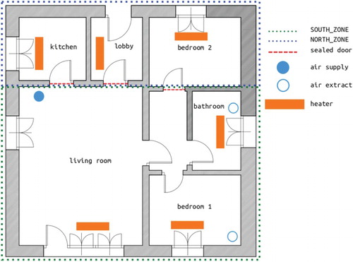
Figure 1 shows the layout of the ground floor wherein the experiment was performed. The attic and basement of the building were considered as boundary spaces, with the internal air temperatures kept constant at . The doors connecting the living room to kitchen, lobby and bedroom 2 were sealed, while ventilation was allowed between the living room, corridor, bathroom and bedroom 1. Blinds were kept closed in the kitchen, lobby and bedroom 2 (NORTH_ZONE) and attic, but were kept open in the living room, corridor, bathroom and bedroom 1 (SOUTH_ZONE). Air leakage was experimentally investigated by performing pressurization tests at the standard pressure difference of 50 Pa.

Figure 1. Twin House O5 – ground floor plan (in colour online).

The experimental schedule was the following:

• Days 1–10: initialization at constant temperature of in SOUTH_ZONE, bedroom 1 and bathroom, and in attic, cellar and NORTH_ZONE.

• Days 11–24: Randomly Ordered Logarithmically distributed Binary Sequence (ROLBS) of heat pulses in SOUTH_ZONE and constant temperature of in attic, cellar and NORTH_ZONE.

• Days 25–31: constant temperature of in SOUTH_ZONE and in attic, cellar and NORTH_ZONE.

• Days 32–40: Freefloat in SOUTH_ZONE, and in attic, cellar and NORTH_ZONE.

This study focuses on the ROLBS phase, in which pseudo-random heat pulses (van Dijk and Tellez 1995) are injected in the SOUTH_ZONE; this is done so that these heat inputs are not correlated with the solar heat inputs. The heating system was composed of lightweight electric heaters with fast response having a split coefficient between convective and radiative heat gains () of 70%/30% according to the manufacturers. The distribution of these devices is shown in Figure 1.

Mechanical ventilation was used during the entire experiment to avoid excessive overheating. The ventilation inlet was in the living room and there were two extraction points in the bathroom and in bedroom 1. The inflow rate was set to and the outflow rates were set to for both extraction points. The ventilation system had ducts going from the basement to the living room and from the living room to the attic.

The provided data set was comprehensive, consisting of 50 variables measured with one-minute time steps. Those employed in the analysis are external temperature, wind speed and direction, internal zone temperatures, zone sensible heat loads, supplied air temperature, basement air temperature, attic air temperature and the ROLBS sequence of heat injections.

3. Model

A detailed ESP-r model was created from the provided experimental specification and on choices and assumptions according to best practice and modeller experience. The building geometry was completely respected as well as the compositions of the construction elements and experimental schedule. The boundary conditions as determined by the external weather were imposed on the model. The resulting BES model was made of seven thermal zones reflecting the different rooms. Since the study focuses on the airflow network sub-model, only the parameters affecting the airflow have been considered. In particular, material properties have been fixed to the values prescribed by the specifications. A diagram of the airflow network model is shown in Figure 2.

Figure 2. Twin House O5 – flow network model (in colour online).

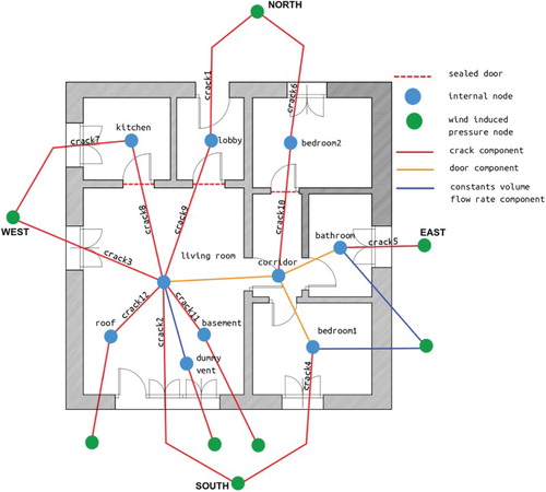
Crack components were used to represent connections between the internal and external environments and between SOUTH_ZONE and NORTH_ZONE. Constant flow rate components were adopted to model the mechanical ventilation system at the supply and extraction points. Bi-directional flow components were employed for the links between the living room, corridor, bathroom and bedroom 1. The resistances of these large openings are very small compared to the other openings, so parameter uncertainties associated with them have been deemed negligible and were neglected in the analysis. For more details regarding the mathematical modelling of the components used to build the flow network model, the reader is referred to Hensen (1991).

4. Uncertainty analysis

As mentioned in Section 1, one feature of this study is the consideration of vectorial (or multidimensional) inputs as well as scalar (or unidimensional) ones.

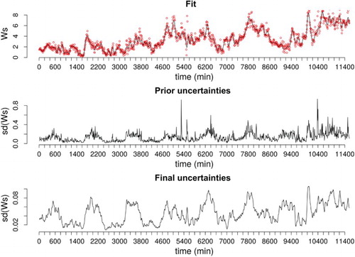
The former consists of variables described by time series and therefore their values change during the experiment and simulations. To adequately characterize the uncertainties for such factors it is necessary to define multidimensional probability distributions depicting time-varying marginal probability distributions and correlation patterns relative to observations at different time steps. Indeed, especially for weather factors such as wind speed (Figure 3), monitoring conditions as well as unobserved phenomena influencing the measurements may result in time-varying magnitudes of the measurement random errors.

Figure 3. Wind speed – smoothing model fit (red dots: observations, black line: model fit), prior uncertainty from Bootstrap and final uncertainties from smoothing.

The multidimensional parameters considered are the following:

• Wind speed, wind direction and external air temperature: these factors are responsible for the main boundary conditions imposed by the exterior environment on the building that affect the airflow. In particular, they determine the pressures at the boundary nodes of the flow network.

• Temperature set-points for the north zones, basement and attic: non-perfect control and systematic and random variability of these variables produce changes in the relative zone pressures thus affecting the ventilation regime.

• ROLBS heat impulses for the south zones: as the main experimental heat inputs, it is expected that these variables have a major influence on the conditions determining ventilation.

To suitably represent the uncertainties of unidimensional model parameters that do not change during the experiment and simulations, it is sufficient to define univariate probability distributions. The parameters of this kind considered are the following:

• Crack dimensions: because of the relatively low infiltration rates, only small cracks have been assumed as connections between the interior and the exterior environments. Their dimensions are sources of uncertainties since they are difficult to measure.

• Wind-induced pressure coefficients: these parameters, together with wind speed, wind direction and ambient air temperature, determine the pressures at the boundary nodes. As they have not been directly observed, they are subject to major uncertainties and one objective of this study is to assess their influence.

• Mechanical ventilation flow rates: particular attention was paid in setting up the experiment to ensure a balance between inflow and outflow from the mechanical ventilation; nevertheless there is the possibility of imbalances due to systematic and random measuring errors which could have a relevant influence on the ventilation regime, so these uncertainties were included in the analysis.

• Ratios between convective and radiative heat gains from ROLBS sequences (): besides possible inaccuracies in these ratios, their values could change because of the particular experimental conditions, zone air temperatures and velocities. For these reasons, they would be better represented by multidimensional probability distributions. However the model allows only constant splits, and thus it was necessary to approximate them with univariate probability density distributions. Variations in these parameters may influence the airflow. In particular, the ratios of convective and radiative gains should determine quicker or slower changes in the zone pressures.

A detailed description of the procedures and assumptions adopted in performing UA for the two different kinds of model inputs follows. The total number of parameters considered was 103 and a summary of the defined uncertainties is in Table 2.

4.1. Multidimensional variables

The measurements are inevitably affected by errors. Two kind of uncertainties are taken into account: systematic and random. The former are intrinsic properties of the sensors used in the monitoring. They can be assumed constant during time or as functions of the measured values and producing always the same bias in the data meaning that a certain sensor always overestimates or underestimates the “true value”. The latter kind of errors is unpredictable and is produced by the stochastic character of the monitored process or by the effects of unobserved phenomena on the measurements. Generally, and in this study, they are assumed to be normally, independently and identically distributed variables.

Under such assumptions, the model assumed for a certain measured variable () including error terms is the following: (1) where is the “true value”, represents systematic errors and indicates random errors.

The properties of would allow the data to be corrected if the exact magnitude and direction of the errors were known. The provided information specified only maximum bounds for such entities and did not allow an accurate evaluation, although all sensors were calibrated as expected in a high-quality experiment. Therefore, their magnitudes and directions were treated as random variables by defining normal distributions with zero mean and standard deviations half the sensor errors estimated during sensor calibration (Table 1). The uncertainties related to systematic errors were simulated by drawing values from these distributions and adding them to the corresponding time series.

Table 1. Systematic sensor errors.

Parameter	Units	Set point	Error
Wind speed	m/s	0–5
Wind speed	m/s
Wind direction	degrees	0–360
Temperatures		30
Ventilation rates		60

Table 2. Considered parameters and relative prior distributions.

Num	Parameter	Type	Units	Initial estimate	Distribution	ID
1	Wind velocity	Multidimensional	m/s
2	Wind direction	Multidimensional	degrees
3	Ambient temperature	Multidimensional
4	Basement temperature	Multidimensional
5	Kitchen temperature	Multidimensional
6	Lobby temperature	Multidimensional
7	Bedroom 2 temperature	Multidimensional
8	Attic temperature	Multidimensional
9	Mech. vent. air temperature	Multidimensional
10	Mech. vent. inflow rate	Univariate		60	N(60, 1.75)
11	Mech. vent. outflow rate bathroom	Univariate		30	N(30, 0.88)
12	Mech. vent. outflow rate bedroom 1	Univariate		30	N(30, 0.88)
13	Lobby external door crack width	Univariate	mm	1
14	Lobby external door crack length	Univariate	m	2.4
15	Living room south window crack width	Univariate	mm	1
16	Living room south window crack length	Univariate	m	7.6
17	Living room west window crack width	Univariate	mm	1
18	Living room west window crack length	Univariate	m	2
19	Bedroom 1 window crack width	Univariate	mm	1
20	Bedroom 1 window crack length	Univariate	m	2
21	Bathroom window crack width	Univariate	mm	1
22	Bathroom window crack length	Univariate	m	2
23	Bedroom 2 window crack width	Univariate	mm	1
24	Bedroom 2 window crack length	Univariate	m	2
25	Kitchen window crack width	Univariate	mm	1
26	Kitchen window crack length	Univariate	m	2
27	Living-kitchen door crack width	Univariate	mm	2
28	Living-kitchen door crack length	Univariate	m	1
29	Living-lobby door crack width	Univariate	mm	2
30	Living-lobby door crack length	Univariate	m	1
31	Corridor-bedroom 2 door crack width	Univariate	mm	2
32	Corridor-bedroom 2 door crack length	Univariate	m	1
33	Living-basement crack width	Univariate	mm	2
34	Living-basement crack length	Univariate	m	1
35	Living-attic crack width	Univariate	mm	2
36	Living-attic crack length	Univariate	m	1
37	Pressure coefficient	Univariate	–	0.7
38	Pressure coefficient	Univariate	–	0.525
39	Pressure coefficient	Univariate	–	0.35
40	Pressure coefficient	Univariate	–	−0.075
41	Pressure coefficient	Univariate	–	−0.5
42	Pressure coefficient	Univariate	–	−0.45
43	Pressure coefficient	Univariate	–	−0.4
44	Pressure coefficient	Univariate	–	−0.3
45	Pressure coefficient	Univariate	–	−0.2
46	Pressure coefficient	Univariate	–	−0.3
47	Pressure coefficient	Univariate	–	−0.4
48	Pressure coefficient	Univariate	–	−0.450
49	Pressure coefficient	Univariate	–	−0.5
50	Pressure coefficient	Univariate	–	−0.075
51	Pressure coefficient	Univariate	–	−0.35
52	Pressure coefficient	Univariate	–	−0.053
101	Living room heater split	Univariate	–	0.7
102	Bedroom 1 room heater split	Univariate	–	0.7
103	Bathroom heater split	Univariate	–	0.7

Note: For pressure coefficients: (1) the angle is referred to the normal direction to the surface, and (2) they are repeated four times (once for each boundary node considered: NORTH, EAST, SOUTH and WEST).

The estimation of random errors is usually done through smoothing methods (Craven and Wahba 1978; Hutchinson and de Hoog 1985; Johnstone and Silverman 1997) and should be based on a priori information about the possible error model, thus avoiding to generate spurious data by excessive smoothing. Establishing a prior error model is not an easy task as the modelled entity is hidden in the data and unpredictable. Useful information about the local precision of the measurements can be gained by evaluating their local variance. In this case, data sampled at high frequency were available, thus it was decided to use Bootstrap (Efron and Tibshirani 1993) to calculate the 10-minute averages from the raw 1-minute time series and to estimate the standard errors relative to these estimates. In this way, it was possible to reduce the simulation burden while keeping an adequate simulation time step and to infer a reasonable prior probability density distribution for the uncertainties () affecting the averaged time series (): (2) (3) (4) where represents an operator that creates a diagonal matrix with elements comprising the given arguments, is the estimated standard error relative to the ith average, is the unknown mean vector and n is the length of .

Then, smoothing with roughness penalty (Ramsay and Silverman 2005) was applied to , with the purposes of inferring , refining the prior error model considered, investigating correlation patterns and providing for missing values in the data. In this framework, measurements are represented through a suitable basis expansion: (5) where are the chosen basis functions, are the corresponding coefficients and is the observation time vector. In this study, B-splines were used as basis functions. It is important to notice that in Equation (5(5) ), the unknown vector has been represented with the function: The smoothing is performed by estimating according to a regularized least-square criterion, penalizing the “roughness” of the data: (6) where λ is a parameter controlling the power of the smoothing and is the matrix quantifying the “roughness”. In this case, it was decided to represent this entity with the curvature of , that is, the square of its second time derivative. This measure of roughness is suggested in Ramsay and Silverman (2005) and is based on the rationale that an infinitely smooth function, like a straight line, has its second derivative always equal to zero, while a highly variable function will show, at least over some ranges, large values for its second derivative. Therefore, is defined as: where indicates the second-order derivative operator and represents the basis system defined by the functions . By minimizing Equation (6(6) ) with respect to , estimates for such variables are given by where .

Thus, in the smoothing, the standard errors calculated through Bootstrap act mostly as weights relative to the accuracies of the values in , so that the smoothing model tries to obtain a closer fit for with low . An example of the uncertainties estimated with the above-explained two-step procedure is provided in Figure 3, for the wind speed. The measurements of this variable were showing high local variability and the uncertainties calculated through Bootstrap appear to overestimate the extent of possible random errors, showing values eight times higher than the respective systematic errors. Refining the error model by smoothing provided values more in agreement with the high monitoring standards characterizing the experiment.

depends on the smoothing parameter λ since the matrix is a function of it. For values of λ close to zero, the model in Equation (5(5) ) tries to fit exactly the observations even if this causes over-fitting. For values of λ approaching ∞, the model will perform a standard linear regression which can be poorly representative of the main dynamical trends. Thus this parameter is particularly important and must be chosen carefully. Ramsay and Silverman (2005) suggest that it is determined in order to minimize the generalized cross validation criterion (GCV): (7) where indicates the trace operator, are the degrees of freedom of the smoothing model and SSE is the sum of squared residuals. GCV can be seen as a discounted mean-squared error measure according to the degree of freedom as a function of λ. The same approach was adopted in this work and the software package described in Ramsay, Hooker, and Graves (2009) was used to carry out the necessary calculations.

Because of the assumption of the noise being Gaussian (Equation (3(3) )), will be normally distributed with mean and covariance matrix . Hence for the property of Gaussian distributions, the following has been assumed for multidimensional variable (Ramsay and Silverman 2005): (8) The probability density distributions defined by Equation (8(8) ) were used to draw random samples for the multidimensional variables. The systematic error terms were then added.

4.2. Unidimensional variables

Most of the univariate variables considered have not been directly observed during the experiment. Thus it was necessary to estimate their uncertainties from indirect measurements, analyst experience and information from literature review. The defined probability distributions describing these parameters are listed in Table 2.

4.2.1. Ventilation flow rate

Ventilation flow rates for mechanically supplied and extracted air were measured during the experiment with one-minute time step. However, the flow network model represents mechanical ventilation inflow and outflow with constant volume flow rate components (Hensen 1991), and it does not allow the use of time-varying flow rates. Therefore, univariate probability distributions were used to summarize the information relating to such variables. A model similar to the one adopted for multidimensional variables was considered: (9) where and indicate a certain volume flow rate and its estimate, s is the systematic error term and ε depicts the random uncertainty. and ε were assessed by bootstrapping the entire time series and s was defined in a similar way as for multidimensional variables, as equal to half the sensor error provided with the experimental specifications (Table 1). The resulting probabilistic model for is (10) (11) where is the variance of the independently and identically distributed variable ε.

Assuming the variance of as indicated in Equation (11(11) ) is a simplification, since random errors will not always be in the same direction as systematic errors. However, estimating from the entire time series produces random uncertainties negligible compared to the systematic ones. In particular, has estimates of and for inflow and outflow, respectively, while s is equal to . Thus even if it results in a slight overestimation of the uncertainties, the assumption in Equation (11(11) ) can be considered reasonable.

4.2.2. Crack lengths and widths

The length and width of the crack components have been evaluated according to the results given by the pressurization test results at 50 Pa. Two blower door tests were performed, one for the whole ground floor and one involving only the SOUTH_ZONE:

• whole ground floor: 1.54 ac/h.

• SOUTH_ZONE: 2.3 ac/h.

The former should give a good picture of the total ground floor infiltration, while the latter represents a mix between infiltration and ventilation between north and south zones. For the two tests, the total leakage area (A) was derived according to the “orifice equation” (Hensen 1991): (12) where is the mass flow rate, is the discharge coefficient, is the air density and is the pressure difference. From the result for the whole ground floor, A has been decomposed relative to NORTH_ZONE and SOUTH_ZONE according to volume proportions. Then from the result regarding only SOUTH_ZONE, it was possible to assess the leakage area responsible for ventilation only, by difference. Crack lengths were estimated depending on opening characteristics and experience and consequently the widths were calculated. Uniform distributions involving ranges of of the estimated values were adopted for these variables.

4.2.3. Wind-induced pressure coefficients

Wind-induced pressure coefficients are possibly the most uncertain variables in the model. No information about their uncertainties came from the experiment and thus suitable probability distributions have been inferred depending upon data from literature review. A complete treatment of their variability would consider the correlation between them, due to their dependence on wind speed, wind direction, location on the surface and configuration of the surrounding area. However, with the available data it was not possible to adequately model such correlation relationships and they have been considered independent. Neglecting the correlation between these model inputs causes overestimation of their uncertainties, whereas considering their interdependence without any specific measurements may lead to the opposite problem. The former option was selected because it was more conservative.

An extensive review of secondary sources of data for pressure coefficients can be found in Costola, Blocken, and Hensen (2009). This study compares pressure coefficient values from different databases depending on different sheltering conditions and derives plausible variation ranges depending on wind directions relative to surface normals. Such information was integrated with the data available from the ESP-r database, including different aspect ratios for walls, in order to define suitable variation ranges. In the flow network model, each boundary nodes is defined by 16 pressure coefficients for wind directions defined every relative to the surface normals. The boundary nodes considered are those named , , and in Figure 2 for a total of 64 pressure coefficients.

4.2.4. Convective/radiative split for heaters ()

In the model only the fractions relating to the convective part were treated as random variables, defining the remaining fractions by difference. An estimate for such variables was given by the heater manufacturer. Therefore, it was considered to be substantially less uncertain than other parameters in the model, and normal probability density distributions with mean 0.7 and standard deviation 0.1 were assumed.

5. Sensitivity analysis

A three-step SA is proposed involving different settings, objectives and methods according to the tasks to perform (Saltelli 2002):

• Factor screening (FS): in this setting the Morris method has been applied to the model in order to gain qualitative information about parameter effect magnitudes and understand which variables may have major influences on the model responses.

• Factor prioritizing (FP) and factor fixing (FF): in this setting the Sobol method, a variance-based SA technique, is used to quantify the amount of variance that can be attributed to individual parameters or group of parameters. This allows the identification of those inputs which should be tuned carefully in order to minimize the model output variance and those inputs which can be fixed to default values because they are responsible for negligible model output variations.

• Factor mapping (FM): in this stage, simulations are weighted according to a chosen criterion and the relative model input vectors are mapped according to their probabilities to produce model realizations close to the target measurements. Furthermore, the importance of the different model parameters that lead to improved calibration is assessed.

FS could be seen as redundant since the same information can be gained from more detailed sensitivity results using FP and FF. However, variance-based methods are particularly simulation intensive and because of the large number of parameters involved (103 in the example considered) the number of simulations needed would have been hardly manageable. Thus it has been deemed appropriate to use the Morris method, which has a substantially lower computational burden, to gather qualitative information and reduce the dimensionality of the problem by grouping together the parameters having small effects. Then the Sobol method has been used to assess the efficacy of the screening.

Usually these methods are applied on scalar model responses. In this study, the model produces vectorial outputs, and it has been necessary to extend the two selected sensitivity techniques by following the principles outlined in Campbell, McKay, and Williams (2006) and Lamboni, Monod, and Makowski (2011). In particular, PCA (Jolliffe 2002) is extensively applied to treat vectorial outputs. Descriptions of the methods used to perform FS, FP, FF and FM with particular emphasis on the modification adopted in order to treat multidimensional outputs follow.

5.1. Factor screening

In this step, the Morris method (Morris 1991) is employed to identify the MIF governing the model in order to reduce its dimensionality to a feasible extent for the next phases. In this phase, model inputs are divided into MIF and least important factors (LIF), and eventually grouped.

The adopted technique characterizes the sensitivity of the model to the ith input, through the concept of elementary effects (), which can be described as partial derivative approximations: where represents the model evaluated at a certain input vector , is a zero vector where only the ith position is equal to one and is the applied variation to the ith input. A chosen number r (usually within the range [20, 50]) of elementary effects are calculated according to a factorial design, representing the parameter space, defined as described in Campolongo, Cariboni, and Saltelli (2007), which allow the needed information to be obtained with a number of simulations (N) linearly proportional to the number of inputs (n): .

The empirical absolute means () and the standard deviations () of the derived samples of characterize, respectively, the magnitude and typology of each input effect. In particular, the magnitudes of first-order effects are proportional to , while parameters having high have significant higher order effects.

To handle the high dimensionality of the ESP-r vectorial outputs, it has been necessary to extend the method. For this purpose PCA was used to decompose the generated simulation data set so that each simulation output () was represented as follows: (13) where Q is the number of retained orthonormal bases and are the principal components. Q has been chosen to explain 99% of the output variance so that represents a negligible amount of the total variability. In this way, the initial data set of dimensionality , where m is the simulation length, has been reduced to Q independent sets of dimensionality suitable to be separately processed by the Morris method, resulting in Q indexes. In particular each simulation output is represented in the space defined by as depicted in Figure 4 where Q has been assumed equal to 3. Thus: (14) where the meaning of is indicated in Figure 4, is the variation applied to the ith input in the jth iteration of the Morris method. A new sensitivity index, , has been defined and used to perform parameter screening as follows: (15) Due to the orthonormality properties of the index can be seen as an approximation of the directional derivative in the gradient direction with respect to the ith input in the reference system defined by PCA. In particular, it is a generalization of the index for vectorial model outputs, and it is representative of the first-order effects of each parameter.

Figure 4. Elementary effect representation in the coordinate system defined by PCA.

The Morris method requires the direct link between one combination of inputs and the associated outputs in order to correctly calculate the elementary effects. Therefore, variations for the multidimensional variables have been generated by taking the iso-probability lines of the inferred distributions (Equation (8(8) )) and considering the defined quantiles as model parameters by including them in the factorial design. The same approach has been used to add systematic errors. This procedure does not produce completely random samples and slightly overestimates uncertainties, since random and systematic errors always add, but it provides adequate variations while keeping the parameters to a reasonable number.

The sensitivity indexes employed in the Morris method can be dependent on the variation ranges applied. In particular, leaving the variations applied to each parameter with its own units can produce misleading results since the calculated elementary affects will have in turn different units, making it impossible to compare them. To avoid this issue model input samples have been scaled and centred so that each of them has mean equal to zero and standard deviation equal to one.

Due to the qualitative character of the results provided by the Morris method, parameter retention is usually done depending on empirical evaluations. In particular, in this case the 10 factors having the highest indexes have been considered sufficient to approximate the original model.

5.2. FP and FF

The purpose of this stage is to extend the qualitative outcomes from the previous analysis by quantifying the amount of model output variance attributable to each model parameter or group of parameters. Through FF the MIF parameters are ranked according to the fraction of model output variance contributed by the parameter. This provides a priority scale for identifying which variables it is necessary to know accurately in order to reduce most of the model output variance. FF provides complementary objectives. In this case, MIF factors are ranked depending on the fraction of model output variance for which they are responsible for including interactions between parameters. This gives information about which factors it is possible to fix to default values because their associated uncertainties have negligible influence on model outputs. In this phase, the effectiveness of the previous parameter screening is assessed by calculating the portion of model output variance attributable to the LIF group. The Sobol method (Sobol 2001) has been used to undertake these tasks. It is based on the decomposition of total (or unconditional) model output variance () into its conditional components. By defining with the ith model input or set of inputs and with its complement, the variance of a variable, , depending on can be decomposed as follows (MacFarlan and Graybill 1963): (16) (17) where and indicate the conditionality of variances () and estimates () on knowing and , respectively.

Equations (16(16) ) and (17(17) ) allow the definition of two sensitivity measures of major importance. In particular, by normalizing these equations by it is possible to derive the two following indexes as fractions of the total output variance (Saltelli et al. 2002): (18) (19) where indicates the portion of which can be attributed to the first-order effect of and is named first-order effect. Parameters with high values for are responsible for most of the output variance, and by knowing their true values it is possible to reduce output uncertainty at least proportionally to the sum of the indexes, since higher order effects might actually contribute as well. This can be seen directly from Equation (16(16) ). Since is a constant, factors with high have low expected output variance ().

represents the portion of left by leaving only unknown, that is, the portion of attributable to all the effects (including first- and high-order effects) of and is called total effect. In particular, setting parameters with negligible to default values should leave a negligible output uncertainty. Similarly if has negligible influence, will be high since for different the estimates of the output are sensibly different and thus assumes small values.

The index is used in performing FP, while the index is employed in carrying out FF. Also, differences in the values of the two indexes indicate how act on the model outputs. For similar and the relative factors have linear and additive effects, while for high and low , they exert their influences by interacting with other inputs or through non-linearities. For example, for linear additive models and while for non-linear models , and since different may account for the same higher order effects.

The multidimensional integrals involved in the evaluation of the estimates and variances in Equations (18(18) ) and (19(19) ) are calculated through Monte Carlo estimation. Several estimators have been proposed to perform this task and a comparison study can be found in Saltelli et al. (2010). In this work, the estimator proposed in Saltelli (2002) was chosen.

As in the previous case the sensitivity indexes described above are defined for scalar model outputs. Their calculation can be extended according to Lamboni, Monod, and Makowski (2011) by using PCA to summarize vectorial model responses. In particular, let be a matrix having as columns the simulation outputs, with centred so that each row has mean equal to 0. Then the total variability of the data set represented by can be defined as the trace () of its empirical covariance matrix ():

It is shown in Lamboni, Monod, and Makowski (2011) that the data set consisting of the sum of the principal components has the same variance as the original data set, and since it is composed of unidimensional variables, it can be used to replace in Equations (18(18) ) and (19(19) ).

In applying the Sobol method, multidimensional inputs were varied by generating random samples from Equation (8(8) ) and then adding the systematic error component. This approach is not subject to uncertainty overestimation.

5.3. Factor mapping

FM is an extension to normal SA which can provide useful information about which parameters it is necessary to focus on in calibration and validation studies. During FS, FP and FF the measures of sensitivity were relative to model output. This may lead to neglecting some variable having a relatively low influence in the model but important for achieving a good fit with the given monitored data. FM, by considering the target measurements as well, provides for this, and integrates the results from the previous phases. It aims to identify input vectors more likely to produce model realizations close to the target observations and thus to determine which model parameters are more powerful in improving the similarity between model predictions and measurements. To perform this task the generalized likelihood uncertainty estimation (GLUE) framework (Beven and Binley 1992) was chosen, in particular the methodology described in Ratto (2001).

GLUE is a simplified Bayesian method allowing inference about posterior estimates of model parameters and model outputs, which is conditional on the measured data. In the usual Bayesian approach, the joint posterior distribution of the model inputs () given the observation set () is defined as (20) where is the likelihood of and is the prior distribution for . It is then possible to infer the posterior estimates and uncertainties for the model inputs and outputs by evaluating the following integrals: (21) (22) (23) (24) where indicates the computer model. Often the evaluations of the integrals in Equations (21(21) )–(24(24) ) are difficult for detailed computer models requiring the employment of Markov chain Monte Carlo or importance sampling methods and the creation of meta-models to speed up the calculations. Additionally the definition of a proper likelihood equation is not always possible due to lack of information.

The GLUE approach assumes that the model parameters are generated directly from their prior distributions and an approximate likelihood measure instead of an accurate one. In particular, a suitable function depending on the sum of squared residuals (SSE) between model realizations and measured data is assumed as an approximation of a proper likelihood measure. Such function weights more model simulations (and thus the relative input vectors) having low SSE and vice versa, and it is called “weighting function” ().

The definition of is problem dependent and examples can be found in Beven et al. (2000). In this study, it has been defined as follows (Ratto 2001): (25) where represents the ith output dependent on , that is, the ith input vector and n is the number of observations. α can be used to regulate the power of the weighting by concentrating higher values of around and is empirically chosen in order to achieve a reasonable distribution of the weights over the simulation sample.

It is then possible to weight each as follows: (26) As Equation (25(25) ) is an approximation of a proper likelihood measure, are approximations of posterior probabilities having drawn the model inputs from their prior probability distributions, and can be used to simplify Equations (21(21) )–(24(24) ): (27) (28) (29) (30) These equations can be estimated through Bootstrap procedures using as sampling weights. Similarly by sampling with replacement the input vectors assuming as sampling probabilities it is possible to infer posterior samples and empirical probability distributions for the model parameters. By analysing differences between the inferred posterior probability distributions and the assumed prior probability distributions, it is possible to assess the importance of each parameter in driving model outputs towards good matches with the target observations since variables most influencing the goodness of the fit will show bigger variations. Thus the value of α is particularly important. Too high a value of this parameter may produce a weight distribution dominated by few , leading to underestimation of the posterior parameter uncertainties. On the other hand, too low a value of α may generate a practically uniform distribution of over the different input vectors, precluding useful information being obtained from subsequent sampling. This parameter has been empirically evaluated and after some trials was set equal to 8.

Similar information can be inferred by processing the values of the weighting function with SA techniques, such as the Sobol method, thus quantifying the importance of the considered model variables in calibrating the computer model. In this case, first-order and total effects represent fractions of (where ). Parameters with high are most responsible for changing the goodness of fit between model outputs and field measurements, that is, are the MIF for model calibration. can be used to assess the variability of the model which could contribute to improve model calibration but that is not considered by neglecting the relative inputs.

Through main and total parameter effects it is also possible to assess the degree of over-parameterization of a model. In particular, big differences between and mean that the goodness of the match between model outputs and measurements is governed by higher order effects and interactions leading to several optimal input vectors. It is important to notice that even if all the parameters are set to their optimal values there still may be discrepancies between simulation results and monitored data, mainly because of model inadequacy. In this case, it may be necessary to improve the model (e.g. through higher resolution modelling), or it may indicate a deficiency in the simulation program.

The main problem with the GLUE method is its slow convergence rate in the estimation of Equations (27(27) )–(30(30) ) if the zones of high probability of the joint posterior distribution is distant from the zones of high probability of the joint prior distribution. In this case, a large number of model simulations is required to achieve a good estimate. This issue is partially mitigated by coupling GSA and GLUE since the former makes available a large set of model outputs which can then be processed by the latter.

If applied in an iterative fashion GLUE can be used to perform model calibration (Beven and Binley 1992), but due to its slow convergence and the empirical character of the adopted measure of goodness of the fit, it is deemed more suitable for preliminary investigation, preceding more rigorous calibration analyses.

6. Results

In the first part of this section, the results for FS, FP and FF are described and a comparison is made between qualitative and quantitative outcomes. In the second part, the results from FM are presented. The model outputs and target data considered are the dry bulb air temperatures for the living room, bedroom 1 and bathroom and the following vector has been considered as model output ():

After parameter screening the identified MIF have been grouped according to parameter typology and all the LIF have been lumped in the LIF group. Thus the relative indexes will represent first-order effects and interaction of the parameters within a group, while will measure also higher order effects between parameters of different groups.

6.1. Factor screening

The results from preliminary FS are depicted in Figure 5, where the first-order effects calculated from the Morris method ( indexes) are shown. In particular, the 10 most important model parameters are highlighted. and are the two most influential variables followed by , , , , , , and which have very similar indexes. These 10 factors have been labelled as MIF and grouped according to the phenomena they represent:

• , have been collected in the parameter;

• , , have been gathered in the parameter;

• and have been grouped in the parameter;

Figure 5. Main effects ( indexes) from the Morris Method for .

while and have been considered separately.

From the results from FF it is also possible to identify the wind direction most influencing the Twin House O5. By rotating the pressure coefficients azimuth angles, in order to refer to the same reference direction, north, the wind coming from direction within the range seems to have the largest effects on the internal temperatures.

6.2. FF and FP

The first-order () and total effects () are listed in Table 3. The model is mainly dominated by first-order effects as the small differences between and indicate. In particular, the sum of the first-order effects is equal to 86% of meaning that about the 14% of is due to higher order effects. Most of the higher order effects can be attributed to interactions between and LIF. They are the only two groups having a noticeable difference between their and .

Table 3. First-order () and total effects () from the Sobol methods for .

Parameter
	0.42	0.46
	0.08	0.16
	0.00	0.00
	0.09	0.08
	0.02	0.02
LIF	0.25	0.31

In the light of this consideration, the higher order effects between the defined group of parameters are negligible. For the total variance, 61% can be attributed to the MIF (most of which is attributable to ), 25% to the LIF and about 14% to interactions, occurring especially between PC and LIF. Thus even if MIF account for the majority of the model variance, still one-third of it is determined by less important factors and their approximation to default values should be undertaken with caution.

6.3. Factor mapping

The model did not provide a particularly good fit of the measured data. In particular, it was able to provide reasonable predictions in the middle part of the ROLBS experiment, but at the beginning and at the end of the heating sequence the simulation outcomes overestimated the observed internal temperatures. This trend is noticeable especially for the living room (Figure 6(a)), while for the bedroom 1 (Figure 6(b)) and the bathroom (Figure 6(c)) the discrepancies between model outputs and measurements are less evident. The main causes are probably model deficiencies lying in the analysed sub-models or in other parts of the overall BES model. In this study, they were investigated by calculating the Pearson correlation coefficient between the residuals and multidimensional model inputs, showing that ROLBS sequences and residuals were moderately correlated (Table 4). The analysis has thus identified an aspect of the model and/or program that needs to be improved in order to get a better match with the measured data.

Figure 6. Comparison between model predictions (black) and observed temperatures (red) (in colour online).

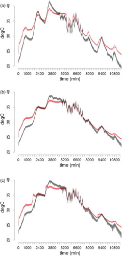
Table 4. Correlation between residuals and ROLBS heating sequences.

Parameter	Living room	Bedroom 1	Bathroom
ROLBS in living room	0.38	0.41	0.42
ROLBS in bedroom 1	0.38	0.41	0.42
ROLBS in bathroom	0.37	0.42	0.51

Figure 7 shows a comparison between prior and posterior probability density distributions, while Table 5 contains the posterior estimates and 95% confidence intervals for the MIF. In particular, the posterior distributions have been generated by sampling with replacement the simulation input vectors using as sampling weights . Even if the prior and posterior variation ranges are substantially the same there are shifts between prior and posterior estimates. The three ratios have estimates very close to their initial values, especially and , while assumes a value slightly higher. Similar considerations can be drawn for the inflow ventilation rate. Its posterior value, although slightly lower, is substantially in agreement with the one inferred from the data. More significant variations between prior and posterior estimates can be observed for crack parameters and pressure coefficients, especially for the latter. Crack lengths assume values about lower than the initial model considered. Pressure coefficients move sensibly from their initial values: increases by , decreases by 89% and increases by 28%.

Figure 7. Comparison between prior (red crosses: quartiles, red dots: averages, blue dots: initial values) and posterior (boxplot) parameter distributions, for MIF. The samples have been normalized between 0 and 1 (in colour online).

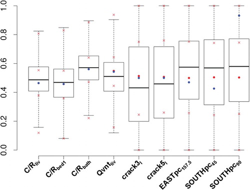
Table 5. Posterior estimates and 95% confidence intervals.

Parameter	Units	Posterior estimate	95% CI
	–	0.72	0.53	0.90
	–	0.71	0.50	0.90
	–	0.71	0.52	0.90
		59.4	54	61.2
	m	1.91	0.85	3.12
	m	1.93	0.87	3.14
	–	−0.20	−0.84	0.32
	–	−0.04	−0.56	0.40
	–	−0.36	−0.97	0.16

One possible cause of significant posterior variance for crack lengths and pressure coefficients can be over-parametrization of the model. This aspect has been analysed by applying the Sobol method to the calculated weights (Table 6). The variance of the weighting function is mostly due to and LIF. This is unexpected since the results from FF and FP were showing that coefficients were responsible by themselves for 42% of the model variance. Additive and linear effects account for the 75% of , so that the remaining 25% can be attributed to higher order effects mainly due to and LIF.

Table 6. First-order () and total effects () from the Sobol method relative to .

Parameter
	0.06	0.08
	0.20	0.39
	0.00	0.00
	0.08	0.12
	0.04	0.07
LIF	0.37	0.49

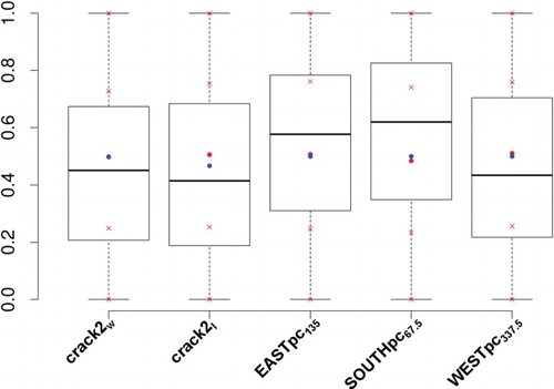
These results indicate that among the LIF there are parameters important for model calibration and validation. Such variables can be identified by comparing their prior and posterior distributions in the same way as was done for the MIF. LIF factors showing significant differences are likely to contribute in a relevant manner to a better match with the measurements. Such comparison is shown in Figure 8 where the variables having the larger differences between their prior and posterior averages are highlighted. These parameters are , , , and

Figure 8. Comparison between prior (red crosses: quartiles, red dots: averages, blue dots: initial values) and posterior (boxplot) parameter distributions for LIF. The samples have been normalized between 0 and 1 (in colour online).

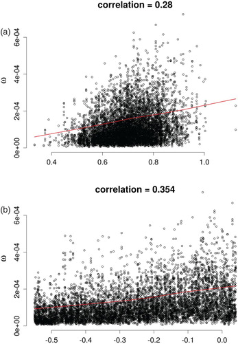
It can also be useful to analyse scatter plots of against the posterior parameter samples and calculate the correlation between them. In this way, it is possible to see how the goodness of the fit changes over the range of variation of each parameter, and to break down groups of factors in order to assess them individually. The latter aspect is particularly helpful in understanding the significantly higher sensitivity that model calibration shows with respect to the pressure coefficients compared to the convective/radiative ratios, which is not in agreement with the results from FP and FF. In particular, this analysis showed that all the pressure coefficients in have relatively significant correlations with the calculated values of the weighting function and comparable with the correlation of , whereas and are only weakly correlated with . Furthermore, the value of the weighting function did not show significant changes over the range of ; therefore, varying this factor does not improve the match with the target data. The scatter plots for the parameters showing higher correlation with are in Figure 9.

Figure 9. trend along parameter posterior variation ranges.

Further investigation could neglect the and focus on the remaining identified factors important for model calibration, namely: , , , , , , , , , and , especially on crack parameters and pressure coefficients. In particular, since the posterior estimates for the coefficients and are quite close to their prior values, these experimental data can be considered accurate. The gained information can be used to reduce prior uncertainties, for example, by replacing the uniform prior distributions of parameters showing significant shifts from their initial values with normal probability density distributions or by setting up prior density distributions favouring parameter values corresponding to higher according to the graphs in Figure 9. However, the latter approach should be used with caution because model over-parameterization can result in more than one set of parameter values giving similar agreement with the measured data. This means that once an input vector is found to give good agreement between model outputs and measurements, moving the parameters as indicated in Figure 9 is likely to produce a similar fit.

7. Conclusions

This paper has demonstrated a multi-step procedure to perform SA on building energy models employing qualitative (Morris method) and quantitative (Sobol method) techniques through their application to a case study. In particular, the explained methodology is particularly apt as a preparatory phase to model calibration and was applied in three phases: FS, FP and FF, and FM. During the first two steps the most influential model parameters were identified and the model variance neglected by considering only these parameters was assessed. The FM stage demonstrated how the output from GSA can be used to gain information aiding subsequent calibration or validation studies by indicating sources of model inadequacy and the model input governing the goodness of fit with the target measured data.

Although the presence of inadequacies in the model may influence the results, it was possible to identify the parameters most responsible for producing good matches with the target data, that is, the pressure coefficients. Thus future investigation should reduce model inadequacy and focus on , , , , , , , , , and , in order to create a model more representative of the real experiment. In particular, ratios between convective and radiative heat gains from the injected ROLBS pulses appear to be particularly important and, although their values should be close to the given specification, in future experiments it may be useful to measure these variables on site. Uncertainties in wind-induced pressure coefficients deserve a more rigorous treatment by accounting for their correlations. On-site measurements as well as wind tunnel experiments could be helpful, although the results from the latter case will be affected by all the limitations of a scaled laboratory experiment.

The comparison between the outcomes of the two sensitivity techniques employed highlight that the LIF are not negligible since they are responsible for relevant fractions of the model and weighting function variances. This is particularly important if SA is preparatory to calibration or validation. In these kinds of studies, it is necessary to single out a few relevant variables. Thus it is important to measure the portion of model variance considered by working only with the retained factors, since MIF certainly have the largest first-order effects. However, the portion of model output variance attributable to them may still be only a relatively small fraction of the total and the LIF, while having negligible first-order effects, may have a combined influence decisive in defining model behaviour. Although caution is needed in drawing general conclusion from particular case studies, it is believed that these considerations may be extended to most BES and thus it is advised, when the additional computational load can be sustained, to employ quantitative techniques to support results from qualitative methods. Furthermore, by extending the analysis with FM, it has been possible to identify further variables (Figure 8) that have significant contributions in improving similarity with target measurement but which were not highlighted by the result from FS, FP and FF.

This last consideration also raises questions about the adequate degree of model detail to adopt especially when model parameters have to be inferred from field observations. Since it is not possible to work considering all the model degrees of freedom, it is believed that high detail should be supported by high-quality information, thus reducing at the outset a great part of parameter uncertainty, and to focus on as few variables as possible. When such high-quality information is not available it would be more convenient to reduce the degrees of freedom of the model from the beginning, by assuming appropriate simplifications during the modelling phase.

Concerning the proposed methodology, novel methods have been introduced for undertaking UA of multidimensional inputs and for considering multidimensional model outputs in the calculation of sensitivity indexes. Multidimensional inputs are rarely considered in sensitivity studies involving BES. Usually, uncertainties are simply represented with a constant offset from a reference vector. This is unrealistic since changing monitoring conditions are likely to produce random errors of different magnitudes. In this work bootstrap and smoothing with roughness penalty techniques have been employed to infer from the large amount of available data plausible multidimensional distributions representing such uncertainties. In this way, it has been possible to investigate how the random variabilities of the observed processes change over time according to the varying monitoring conditions. It is hard to assess the correctness of uncertainty quantification. However, it is believed that such an approach is more sensible and rigorous than the common practice, leading to more realistic estimates of the uncertainties for multidimensional model inputs. To check this, FS was also performed considering constant uncertainties for multidimensional variables. A constant variance equal to the average of the estimated variances using the bootstrap technique was assumed for these parameters and the results are presented in Figure 10. Comparing this with Figure 5, the same parameters still have the most influence, but the relative order of importance has changed, so that is the dominant parameter when constant uncertainty is assumed. Thus particularly when a substantial amount of information is available, it is advisable to employ advanced statistical techniques like those used in order to perform UA.

Figure 10. FS results by considering constant uncertainties for multidimensional variables.

The information about the sensitivity of a certain model output to the inputs should be concise and at the same time be comprehensive. When the output in question is vectorial, the achievement of these two objectives is not easy. Common practice involves calculating sensitivity indexes for each time step of the simulation or the utilization of functional-like integrals or distance measures from reference values in order to reduce the simulation vectors to scalars. While the former approach produces redundant and difficult to summarize information, the latter neglects the dynamic trends of the vectorial output. Here PCA has been used to complement the Morris and Sobol methods to effectively deal with vectorial outputs and return concise and easy to interpret information in the form of a few significant sensitivity indexes that represent the model response. In particular, a new expansion of the Morris method has been proposed in order to treat vectorial model outputs. PCA was used to project the model outputs in a convenient reference space and a new sensitivity index, M, was defined. Results carried out with the new approach were substantially in agreement with those from the Sobol method.

In more practical case studies, it is necessary to consider multiple performance indicators since design problems are often multi-objective. The proposed methodology can easily be extended in that sense by clearly defining a hierarchy among the different indicators. For example, a weighting function of the sensitivity indexes calculated for the different performance metrics can serve this purpose. This will be explored in future work.

It is believed that the methodology employed in this study forms a rigorous basis for undertaking SAs and in reducing the degrees of freedom of BES models in a more informative way, which is superior to the common practice based on qualitative screening, especially if employed as a preparatory stage to calibration or validation. In particular, it should become good practice to quantify the amount of variance attributable to the retained inputs in order to adequately justify model simplifications. As shown, LIF parameters govern about 30% of the model variability and about 50% of the variability of weighting function, and a subsequent calibration or validation study should extend the MIF parameters with the variables identified by FM. This latter step of the methodology is particularly effective in complementing the result from GSA and justifies the additional computational load required in quantifying parameter effects. The effectiveness of the method has been demonstrated in a particular sub-model but a comprehensive analysis should consider the overall BES model.

Acknowledgements

The authors acknowledge support from the Engineering and Physical Sciences Research Council (Ref: EP/K01532X/1).

Disclosure statement

No potential conflict of interest was reported by the authors.

Funding

Results were obtained using the EPSRC funded ARCHIE-WeSt High Performance Computer (www.archie-west.ac.uk): EPRSC grant no. EP/K000586/1.

References

- Aude, P., L. Tabary, and P. Depecker. 2000. “Sensitivity Analysis and Validation of Buildings Thermal Models Using Adjoint-Code Method.” Energy and Buildings 31 (3): 267–283. http://dx.doi.org/10.1016/S0378-7788(99)00033-X. doi: 10.1016/S0378-7788(99)00033-X
- Beven, K., and A. Binley. 1992. “The Future of Distributed Models: Model Calibration and Uncertainty Prediction.” Hydrological Processes 6 (3): 279–298. http://dx.doi.org/10.1002/hyp.3360060305. doi: 10.1002/hyp.3360060305
- Beven, K., J. Freer, B. B Hankin, and K. Schultz. 2000. “The Use of Generalised Likelihood Measures for Uncertainty Estimation in High Order Models of Environmental Systems.” In Nonlinear and Nonstationary Signal Processing, edited by, W. J. Fitzgerald, R. L. Smith, A. T. Walden and P. C. Young. Cambridge University Press.
- Booth, A.T., and R. Choudhary. 2013. “Decision Making under Uncertainty in the Retrofit Analysis of the UK Housing Stock: Implications for the Green Deal.” Energy and Buildings 64: 292–308. http://dx.doi.org/10.1016/j.enbuild.2013.05.014. doi: 10.1016/j.enbuild.2013.05.014
- Bucking, S., R. Zmeureanu, and A. Athienitis. 2013. “A Methodology for Identifying the Influence of Design Variations on Building Energy Performance.” Journal of Building Performance Simulation 7 (6): 411–426. http://dx.doi.org/10.1080/19401493.2013.863383. doi: 10.1080/19401493.2013.863383
- Campbell, K., M. D. McKay, and B. J. Williams. 2006. “Sensitivity Analysis When Model Outputs Are Functions.” Reliability Engineering & System Safety 91 (10–11): 1468–1472. http://dx.doi.org/10.1016/j.ress.2005.11.049. doi: 10.1016/j.ress.2005.11.049
- Campolongo, F., and R. Braddock. 1999. “The Use of Graph Theory in the Sensitivity Analysis of the Model Output: A Second Order Screening Method.” Reliability Engineering & System Safety 64 (1): 1–12. http://www.sciencedirect.com/science/article/pii/S0951832098000088. doi: 10.1016/S0951-8320(98)00008-8
- Campolongo, F., J. Cariboni, and A. Saltelli. 2007. “An Effective Screening Design for Sensitivity Analysis of Large Models.” Environmental Modelling & Software 22 (10): 1509–1518. http://linkinghub.elsevier.com/retrieve/pii/S1364815206002805. doi: 10.1016/j.envsoft.2006.10.004
- Cipriano, J., G. Mor, D. Chemisana, D. Prez, G. Gamboa, and X. Cipriano. 2015. “Evaluation of a Multi-stage Guided Search Approach for the Calibration of Building Energy Simulation Models.” Energy and Buildings 87: 370–385. http://www.sciencedirect.com/science/article/pii/S0378778814009013. doi: 10.1016/j.enbuild.2014.08.052
- Clarke, J. 2001. Energy Simulation in Building Design. Oxford: Butterworth-Heinemann.
- Corrado, V., and H. E. Mechri. 2009. “Uncertainty and Sensitivity Analysis for Building Energy Rating.” Journal of Building Physics 33 (2): 125–156. http://jen.sagepub.com/cgi/doi/10.1177/1744259109104884. doi: 10.1177/1744259109104884
- Costola, D., B. Blocken, and J. L. M. Hensen. 2009. “Overview of Pressure Coefficient Data in Building Energy Simulation and Airflow Network Programs.” Building and Environment 44 (10): 2027–2036. http://dx.doi.org/10.1016/j.buildenv.2009.02.006. doi: 10.1016/j.buildenv.2009.02.006
- Craven, P., and G. Wahba. 1978. “Smoothing Noisy Data with Spline Functions.” Numerische Mathematik 31 (4): 377–403. http://dx.doi.org/10.1007/BF01404567. doi: 10.1007/BF01404567
- van Dijk, H. A. L., and F. M. Tellez. 1995. Measurement and Data Analysis Procedures, Final Report of the JOULE II COMPASS Project (JOU2-CT92-0216). Technical Report.
- Efron, B., and R. J. Tibshirani. 1993. An Introduction to the Bootstrap. New York: Chapman & Hall.
- Eisenhower, B., Z. ONeill, V. A. Fonoberov, and I. Mezic. 2012. “Uncertainty and Sensitivity Decomposition of Building Energy Models.” Journal of Building Performance Simulation 5 (3): 171–184. http://dx.doi.org/10.1080/19401493.2010.549964. doi: 10.1080/19401493.2010.549964
- Sanchez, D. G., B. Lacarrière, M. Musy, and B. Bourges. 2014. “Application of Sensitivity Analysis in Building Energy Simulations: Combining First- and Second-Order Elementary Effects Methods.” Energy and Buildings 68: 741–750. doi: 10.1016/j.enbuild.2012.08.048
- Hensen., J. L. M. 1991. “On the Thermal Interaction of Building Structure and Heating and Ventilating System.” Ph.D. thesis. Technische Universiteit Eindhoven.
- Heo, Y., G. Augenbroe, and R. Choudhary. 2013. “Quantitative Risk Management for Energy Retrofit Projects.” Journal of Building Performance Simulation 6 (4): 257–268. doi: 10.1080/19401493.2012.706388
- Heo, Y., R. Choudhary, and G. A. Augenbroe. 2012. “Calibration of Building Energy Models for Retrofit Analysis under Uncertainty.” Energy and Buildings 47: 550–560. doi: 10.1016/j.enbuild.2011.12.029
- Hopfe, C. J., and J. L. M. Hensen. 2011. “Uncertainty Analysis in Building Performance Simulation for Design Support.” Energy and Buildings 43 (10): 2798–2805. http://dx.doi.org/10.1016/j.enbuild.2011.06.034. doi: 10.1016/j.enbuild.2011.06.034
- Hutchinson, M. F., and F. R. de Hoog. 1985. “Smoothing Noisy Data with Spline Functions.” Numerische Mathematik 47 (1): 99–106. http://dx.doi.org/10.1007/BF01389878. doi: 10.1007/BF01389878
- IEA EBC Annex 58. 2011–2015. “Reliable Building Energy Performance Characterisation Based on Full Scale Dynamic Measurements.” IEA EBC Annex 58. http://www.ecbcs.org/annexes/annex58.htm.
- Johnstone, I. M., and B. W. Silverman. 1997. “Wavelet Threshold Estimators for Data with Correlated Noise.” Journal of the Royal Statistical Society. Series B (Methodological) 59 (2): 319–351. http://www.jstor.org/stable/2346049. doi: 10.1111/1467-9868.00071
- Jolliffe, I. T. (2002). Principal Component Analysis, Springer Series in Statistics. New York: Springer.
- Kim, Y. J., K. C. Kim, C. S. Park, and I. H. Kim. 2014. “Deterministic vs. Stochastic Calibration of Energy Simulation Model for an Existing Building.” ASim 2014, IBPSA Asia Conference, Nasoga, Japan, November.
- Lamboni, M., H. Monod, and D. Makowski. 2011. “Multivariate Sensitivity Analysis to Measure Global Contribution of Input Factors in Dynamic Models.” Reliability Engineering & System Safety 96 (4): 450–459. http://dx.doi.org/10.1016/j.ress.2010.12.002. doi: 10.1016/j.ress.2010.12.002
- Macdonald, I., and P. Strachan. 2001. “Practical Application of Uncertainty Analysis.” Energy and Buildings 33 (3): 219–227. http://dx.doi.org/10.1016/S0378-7788(00)00085-2. doi: 10.1016/S0378-7788(00)00085-2
- MacFarlan, M. A., and F. A. Graybill. 1963. Introduction to the Theory of Statistics. 2nd ed. New York: McGraw-Hill.
- Morris, M. D. 1991. “Factorial Sampling Plans for Preliminary Computational Experiments.” Technometrics 33 (2): 161–174. http://dx.doi.org/10.2307/1269043. doi: 10.1080/00401706.1991.10484804
- Ramsay, J. O., G. Hooker, and S. Graves. 2009. Functional Data Analysis with R and MATLAB. 1st ed. Springer.
- Ramsay, J. O., and B. W. Silverman. 2005. Functional Data Analysis. 2nd ed. New York: Springer.
- Ratto, M. 2001. “Sensitivity Analysis in Model Calibration: GSA-GLUE Approach.” Computer Physics Communications 136 (3): 212–224. http://dx.doi.org/10.1016/s0010-4655(01)00159-x. doi: 10.1016/S0010-4655(01)00159-X
- Reddy, T. A., I. Maor, and C. Panjapornpon. 2007a. “Calibrating Detailed Building Energy Simulation Programs with Measured Data – Part II: Application to Three Case Study Office Buildings (RP-1051).” HVAC & R Research 13 (2): 221–241. doi: 10.1080/10789669.2007.10390952
- Reddy, T. A., I. Maor, and C. Panjapornpon. 2007b. “Calibrating Detailed Building Energy Simulation Programs with Measured Data – Part I: General Methodology (RP-1051).” HVAC & R Research 13 (2): 243–265. doi: 10.1080/10789669.2007.10390953
- Rysanek, A. M., and R. Choudhary. 2013. “Optimum Building Energy Retrofits under Technical and Economic Uncertainty.” Energy and Buildings 57: 324–337. http://dx.doi.org/10.1016/j.enbuild.2012.10.027. doi: 10.1016/j.enbuild.2012.10.027
- Saltelli, A. 2002. “Making Best Use of Model Evaluations to Compute Sensitivity Indices.” Computer Physics Communications 145 (2): 280–297. http://dx.doi.org/10.1016/s0010-4655(02)00280-1. doi: 10.1016/S0010-4655(02)00280-1
- Saltelli, A., P. Annoni, I. Azzini, F. Campolongo, M. Ratto, and S. Tarantola. 2010. “Variance Based Sensitivity Analysis of Model Output. Design and Estimator for the Total Sensitivity Index.” Computer Physics Communications 181 (2): 259–270. http://www.sciencedirect.com/science/article/pii/S0010465509003087. doi: 10.1016/j.cpc.2009.09.018
- Saltelli, A., S. Tarantola, F. Campolongo, and M. Ratto. 2002. Sensitivity Analysis in Practice: A Guide to Assessing Scientific Models. Wiley-Blackwell. http://dx.doi.org/10.1002/0470870958.
- Sobol, I. M. 2001. “Global Sensitivity Indices for Nonlinear Mathematical Models and their Monte Carlo Estimates.” Mathematics and Computers in Simulation 55 (1–3): 271–280. http://dx.doi.org/10.1016/S0378-4754(00)00270-6. doi: 10.1016/S0378-4754(00)00270-6
- Spitz, C., L. Mora, E. Wurtz, and A. Jay. 2012. “Practical Application of Uncertainty Analysis and Sensitivity Analysis on an Experimental House.” Energy and Buildings 55: 459–470. http://dx.doi.org/10.1016/j.enbuild.2012.08.013. doi: 10.1016/j.enbuild.2012.08.013
- Strachan, P., F. Monari, M. Kersken, and I. Heusler. 2015a. “IEA Annex 58: Full-scale Empirical Validation of Detailed Thermal Simulation Programs.” 6th international building physics conference, IBPC, Torino, Italy, June.
- Strachan, Paul, Katalin Svehla, Ingo Heusler, and Matthias Kersken. 2015b. “Whole Model Empirical Validation on a Full-Scale Building.” Journal of Building Performance Simulation 1–20. http://dx.doi.org/10.1080/19401493.2015.1064480. doi: 10.1080/19401493.2015.1064480
- Sun, J., and T. A. Reddy. 2006. “Calibration of Building Energy Simulation Programs Using the Analytic Optimization Approach (RP-1051).” HVAC&R Research 12 (1): 177–196. doi: 10.1080/10789669.2006.10391173
- Tian, Wei. 2013. “A Review of Sensitivity Analysis Methods in Building Energy Analysis.” Renewable and Sustainable Energy Reviews 20: 411–419. http://dx.doi.org/10.1016/j.rser.2012.12.014. doi: 10.1016/j.rser.2012.12.014