Occupant behaviour modelling in domestic buildings: the case of household electrical appliances

Abstract

This paper presents a new approach to bottom-up stochastic occupant behaviour modelling for predicting the use of household electrical appliances in domestic buildings. Three metrics relating to appliance occupant behaviours are defined: the number of switch-on events per day, the switch-on times and the duration of each appliance usage. The metrics were calculated for 1,076 appliances in 225 households from the UK Government’s Household Electricity Survey carried out in 2010–2011. The analysis shows that occupant behaviour varies substantially between households, across appliance types and over time. The new modelling approach improves on previous approaches by using a three-step process where the three-appliance occupant-behaviour metrics are simulated respectively using stochastic processes to capture daily variations in appliance occupant behaviour. It uses probability and cumulative density functions based on individual households and appliances which are shown to have advantages for modelling the variations in appliance occupant behaviours.

Keywords:

• appliance behaviour
• occupant behaviour
• household electrical appliances
• stochastic modelling
• data-driven modelling
• bottom-up modelling

1. Introduction

Occupant behaviour in buildings can be defined as both the occupant presence and the occupant actions that may influence the building environmental conditions and the building energy consumption (Yan and Hong 2014). These include the occupants’ operation of windows, air conditioning systems and heating systems (such as window opening, timer settings and choice of thermostat set-points) that affect hygrothermal conditions, indoor air quality, light, noise and temperature (Guerra Santin, Itard, and Visscher 2009; Hoes et al. 2009; Schweiker et al. 2012). It also includes the use of services within the building, such as hot water, cooking and electrical appliances, which consume energy and generate internal heat gains (Isaksson and Karlsson 2006; Yamaguchi, Fujimoto, and Shimoda 2011).

Occupant behaviour is an increasingly important area in building performance simulation and is widely recognized as a major uncertainty factor in building performance (Yan et al. 2015). Studies which model the occupants’ interaction with buildings and control systems have included lighting controls (Reinhart et al. 2006), shading devices (Haldi and Robinson 2010) and ventilation (Yun et al. 2008). Other studies have focused on occupancy presence, fundamental for occupancy research as most occupant behaviour patterns are influenced by occupancy (Roetzel et al. 2010; D’Oca and Hong 2014; Zhao et al. 2014; Feng et al. 2015). Characterising the stochastic nature of occupant behaviour has proved to be non-trivial and previous researchers have identified several constraints to progress including the lack of a common modelling approach, the lack of a rigorous model validation framework, the lack of experimental designs and the lack of suitable monitoring data with which to develop models (Yan and Hong 2014; Yan et al. 2015).

The use of electrical appliances is important for understanding occupant behaviour in domestic buildings (Swan and Ugursal 2009; Grandjean, Adnot, and Binet 2012). Household electrical appliances include all those appliances typically found in homes such as ‘wet’ appliances (washing machines, tumble dryers, dishwashers), ‘cold’ appliances (fridges, freezers), televisions, cooking appliances, electric showers and many more. Using electrical appliances impacts on the timing and magnitude of a household’s overall electricity consumption and, more importantly for building thermal simulation studies, on the timings and magnitude of internal heat gains within the building. The occupant behaviours of interest include: the time of day when occupants switch on the appliances, the frequency of appliance use, the length of time for which the appliance is switched on, the choice of power mode or cycle programme and the potential for interaction between the use of difference appliance types (for example, a tumble dryer may be switched on following the use of a washing machine). Occupant behaviour models of household electrical appliance use have been used in many applications, including the planning the integration of local energy systems and emerging technologies (Yao and Steemers 2005; Widén and Karlsson 2010) and the better prediction of time variations of power demand and peak demand to analyse the impact of energy efficiency schemes or demand response on the network load flows (Paatero and Lund 2006; Yamaguchi, Fujimoto, and Shimoda 2011). In addition, predicting the internal heat gains from appliances in zero carbon buildings is becoming increasingly important as studies have shown that they have a significant effect on energy consumption and overheating in passive buildings (Hoes et al. 2009).

Researchers have developed a number of stochastic appliance use models to integrate with simulation tools in order to include the randomness linked to the variation in occupant behaviour between households and the variation in time of each behaviour. Typically, these models are based on one-day diaries, from Time of Use (TOU) surveys, reporting households’ daily activities of 5000–10,000 households (Tanimoto, Hagishima, and Sagara 2008; Richardson et al. 2010; Widén, Molin, and Ellegård 2012; Wilké et al. 2013). There are also long-term observational studies where appliances were monitored for extended periods using electrical power sensors (Page 2007). The studies that used TOU data obtained the switch-on times and duration of appliance use from user diaries which are then converted to appliance power demands with fixed power demand profiles. The occupancy behaviour patterns associated with different types of households and days are analysed to develop the model. In this approach, the switch on times cannot be identified precisely as users write down their daily activities each 10 or 15 minutes. Another limitation is that one-day diary-based TOU datasets fail to capture the difference in behaviour for an extended period of time and difference in durations/choice of programme between usages. Other studies analysed measured data to obtain the switch-on times, duration and the power demand profiles. The limitation of these long-term studies is that, due to the high cost of monitoring, the sample size is relatively small (2–10 homes) and thus cannot be considered representative for a population or able to capture behavioural diversity among different groups. As a consequence of the challenges of modelling occupant behaviour, the occupants’ use of household electrical appliances is often modelled as fixed static schedules in building simulation tools such as DOE-2, BLAST and EnergyPlus (Abushakra and Claidge 2001; Hoes et al. 2009). However, such procedures can lead to overestimated peak values, as defining standard behaviour for types of households fails to consider the random variability of the occupant behaviour (Tanimoto and Hagishima 2010).

This paper develops new insights into appliance behaviour modelling for household electrical appliance use. The term ‘appliance behaviour’ is defined here as a combination of occupant behaviour and the operating characteristics of the appliance itself. In this work, three appliance behaviour metrics are proposed to describe the behaviour of household electrical appliance use: (i) the number of switch-on events that occur over a specified time period (e.g. a day or a month); (ii) the time of day when each switch-on event occurs; and (iii) the duration of appliance use (the length of time that the appliance is switched on for). In some cases, an appliance behaviour is directly driven by the occupant behaviour (e.g. switching on a television); in other cases, appliance behaviour is determined solely by the appliance (e.g. a fridge cycling on and off when the occupants are not at home) and in some cases, a combination of both occupant behaviour and appliance characteristics determines the appliance behaviour (e.g. the duration of a washing machine cycle is determined both the user’s choice of programme cycle and the make and model of the machine itself). The distinction between occupant behaviour and appliance characteristics is discussed further in Section 3.1.

This work studies the development and application of different modelling techniques using one of the most comprehensive datasets of household appliance usage recorded to date: the UK Government’s ‘Household Electricity Survey’ (HES) (DECC 2014a). The HES took place in 2011 and, for periods of either one month or one year, recorded the electricity consumption of 5860 household electrical appliances in 251 homes. The HES dataset is first analysed to identify and quantify the three-appliance behaviour metrics for 225 homes in the sample which were monitored for a one-month period. The analysis focuses on the main appliance types found in homes and studies 16 household appliance types in the 225 homes (1076 appliances in total). Occupant behaviour models are developed (based on a probability density function (pdf) approach) and used to run stochastic simulations of the occupant behaviour within the HES homes. Two approaches to modelling the appliance behaviour metrics are tested in this paper. Approach 1 takes a simple approach often used in appliance behaviour modelling in literature whereas Approach 2 takes a different approach designed to improve the accuracy of modelling in terms of the daily number of switch-on events. Results from the simulations are analysed and compared to evaluate the strengths and limitations of the proposed models and provide insights into the future development of occupant behaviour modelling techniques based on monitored data. The paper concludes with a discussion of the future research directions for appliance occupant behaviour modelling methodologies (including statistical analysis, probabilistic modelling and validation approaches) and of the design of future monitoring studies to fully capture household appliance usage (including monitoring strategies and sample sizes).

2. Household electricity survey dataset

2.1. Background

In 2011, the UK Government carried out a major survey of the use of household electrical appliances in homes. The Household Electricity Survey 2011 (HES 2011) recorded the electric power demand of 251 UK homes and 5860 individual electrical appliances within those homes. The complete dataset has been made publically available by the Department of Energy and Climate Change (the details on accessing the publicly available dataset are provided at the end of this paper). The dataset is one of the most comprehensive recorded to date, and has resulted in several reports detailing the usage of appliances in homes. All households were owner-occupied and the survey households were selected on the basis of the life-stage of the occupants, including single pensioners & non-pensioners, multiple pensioner, families and multiple persons with no children (DECC 2014a).

Table 1 gives a summary of the data that were collected during the HES survey. The appliances were numbered, according to their type from 1 to 250. The electrical power of most of the individual appliances (cold, wet and small appliances) was measured using serial wattmeters developed by Enertech which were directly plugged into the wall sockets and the household appliance to be monitored was connected to the trailing socket of the wattmeter. Appliances such as water heating and cooking appliances were monitored directly from the consumer unit of the house using the Multivoies™ system which was installed inside the consumer unit (DECC 2014a).

Table 1. Summary of the variables that were monitored/collected in the Household Electricity Use Survey.

Variable	Description
Power demand	The electrical power demand of 5,680 appliances in 251 homes with a mix of 2- and 10-minute resolution recording interval
	225 homes were monitored at 2-minute resolution for time periods of around a month
	26 homes were monitored at 10-minute resolution for time periods of around a year
Appliance characteristics	Brand manufacturer – model of the appliance
	Year of the product bought with their energy efficient ratings
Diaries	Diary data collected for households’ use of certain appliances. Most households completed diaries for two weeks
Demographics and household characteristics	Household types, household age, working status
	UKHES code
	Answers to the environmental attitude questionnaires
Temperature	The internal and external temperatures of the house were monitored using thermometers
Details of house dimension and construction	Dwelling types
	Floor area and window area
	Glazing type Insulation thickness

The resulting dataset contains the power demand of the individual appliances recorded at a mix of 2-minute and 10-minute resolutions. In addition, an appliance survey recorded the age, brand and other details of the appliances. Participants were also asked to keep detailed diaries for two weeks of how they used certain appliances such as washing machines (e.g. the wash temperature, choice of programme, fullness of the machine) and hobs (e.g. hob settings: low, medium, high). Further data collected in the HES were not used in the analysis presented here. This included attitude questionnaires, internal and external temperature measurements and detailed information about the house characteristics such as the dimensions and construction materials.

2.2. Data selection, cleaning and processing

Figure 1 shows the monitoring periods of the 225 homes selected from the HES dataset for analysis in this work. A subset of the full dataset of 251 homes was chosen as different measurement intervals were used in the survey (2-minute and 10-minute intervals) and this work considers only the 225 homes which had their appliance power measurements recorded at 2-minute intervals. This shorter time interval provides the greatest level of detail for identifying the occupant behaviours and means the subsequent analysis and modelling methods provided in this paper were based on the same measurement interval for all homes. In Figure 1, the monitoring periods for the 225 homes are shown in order of start date, with the horizontal line for each home denoting the start and end of the monitoring period when appliance power measurements were taken. All monitoring took place between May 2010 and June 2011 on a rolling basis, with different homes monitored at different time periods between these dates. This was done so that the monitoring equipment could be re-used for different homes during the survey. The homes were monitored for between 20 and 45 days, with an average monitoring period of 27.7 days.

Figure 1. The monitored periods (start date to end date) of the 225 homes in the HES dataset studied in this work. All the homes here have appliance power measurements recorded at 2 minute intervals.

Figure 2 shows the frequency distribution of the 16 appliance types in the 225 homes. In total, 1076 appliances were analysed. These 16 appliance types were chosen due to their high ownership rates and because they have a significant impact on buildings’ electricity demand, representing, on average, 75% of the annual electricity consumption in a UK home (DECC 2014a, 2014b). The 16 appliance types also represent different modes of occupant interaction and different modes of appliance operation, and hence require different modelling approaches. For wet appliances, occupants are actively involved in loading them before switching them on but there is no interaction with the appliance while the cycle is running. For cold appliances, the user does not need to switch it on and off after the initial set up and they are in use continuously. For cooking appliances and electric showers, the user directly chooses the time when the appliance is switched on and the length of time it is used for.

Figure 2. Number of appliances analysed for this study monitored in the HES (2011) (TV1 is the first mainly watched television, TV2 is the second most frequently used television and TV3 is the third most frequently used television).

Figure 2 shows that the most common appliance type in the sample was washing machines (n = 176), followed by fridge-freezers (n = 129) and electrical cookers (n = 105) which consist of a hob, oven and grill. The least common appliance types were electric grills (n = 5) and electric hobs (n = 9). Although hobs and grills are found in the majority in UK homes, in most cases, they are operated by gas rather than electricity (DECC 2014a).

Data cleaning was carried out on the 2-minute appliance power measurements prior to analysis. Visual inspection of time series plots was used to identify incorrect readings. About 0.006% of the power measurements were identified as incorrect readings and these were removed from the dataset. Where there was a significant part of the day missing, the whole day was deleted so as not to distort statistics based on daily usage. Where a small number of consecutive readings (up to 4 minutes) were missing, the missing data points were manually inserted by using linear interpolation between the adjacent values. About 0.002% of the data were estimated in this manner. Given that all the data cleaning modifications involved only a very small percentage of the overall data readings collected, it is expected that impact on the analysis and the results would be minimal.

3. Appliance behaviour metrics

3.1. Choice of appliance behaviour metrics

A review of the literature identified a number of occupant behaviours for household appliance usage including switch-on times, usage durations, choice of power mode for the appliance operation and behaviour towards stand-by (Capasso et al. 1994; Paatero and Lund 2006; Page 2007; Richardson et al. 2010; Widén et al. 2011; Yamaguchi, Fujimoto, and Shimoda 2011; Wilké et al. 2013).

Table 2 summarizes the appliance behaviour metrics chosen for this study based on the literature review and includes the metric definitions, to which appliance type they are applied and the influencing factors of occupant behaviour and appliance characteristics. There are three appliance behaviour metrics identified for this study: (1) number of switch-on events is the count of switch-on events that occur over a specified time period; (2) switch-on time of day is the times when the switch-on events occur; and (3) duration is the length of time for which the appliance is used. Here a switch-on event is defined as the start of the use of an appliance and is considered as a time-dependent quantity. Duration is defined as the period between the switch-on and either switch-off or stand-by event. Standby use occurs when an appliance is not in use but is still consuming power (Cogan et al. 2006). Consumer electronic equipment such as televisions and set-top boxes have standby mode in which the occupant can leave appliances on stand-by or switch them completely off (Firth et al. 2008). Appliance behaviour is defined at a household level (rather than an individual level), as it is only possible from the sensor measurements to track when appliances are switched on, not by whom, making it impossible to determine an individual occupant’s activities. For wet appliances, occupants are actively involved in loading and starting the appliance (the switch-on times) but do not directly choose the duration or switch-off times. Although there is no interaction with the user while running, as the power demand and duration of the cycle are highly dependent on the washing temperature and the amount of water needed, occupant behaviour is a significant factor through the choice of the washing machine programme. Televisions, cooking appliances and showers are actively switched on or off by the occupants. The duration of these appliances is directly related to the activities of the occupants. Cold appliances are in use continuously and the user has no direct interaction with the switch-on or switch-off times; however, the duration is affected by occupant’s door opening or storing food inside.

Table 2. Appliance behaviour metrics.

Appliance behaviour metric^a	As applies to:	Definition	Occupant behaviour influencing factors	Appliance characteristics influencing factors
Metric 1: Number of switch-on events	Wet appliances, cooking appliances, TVs, electric showers	The number of times in a specific time period that the appliance is switched on	Occupancy patterns and occupant use of appliances	None
	Cold appliances	The number of times in a specific time period that the compressor switches on	The occupant setting of the internal thermostat, number of times the door is opened, amount of contents (food) in the appliance	Appliance’s own cooling mechanism for temperature control
Metric 2: Switch-on time of day	Wet appliances, cooking appliances, TVs, electric showers	The time of day when the appliance is switched on by the user	As above	None
	Cold appliances	The time of day when the compressor switches on	As per ‘switch-on number’ above	As above
Metric 3: Duration	Wet appliances	The length of time which the chosen appliance cycle runs	Choice of cycle, amount of clothes/dishes placed in device	Impact of make/model of appliance on cycle duration, cold water feed temperature
	Cooking appliances, TVs, electric showers	The length of time until the user switches off the appliance.	Occupancy patterns and occupant use of appliances	None
	Cold appliances	The length of time which the compressor runs for	As per ‘switch-on times’ above	As per ‘switch-on times’ above plus impact of make/model of appliance on compressor cycling

^aAppliance behaviour is used as a combination of occupant behaviour and appliance characteristics.

3.2. Identifying appliance behaviour metrics in the monitored data

The three-appliance behaviour metrics in Section 3.1 were inferred from the 225 HES households using the monitored 2-minutely power demand measurements. Microsoft Access 2013 and Matlab were used to identify the metrics and analyse the data. Figure 3 illustrates the identification method for the switch-on and switch-off times from the power demand measurements for three appliance types: a washing machine cycle with the high peak at the start and an increase at the end of the cycle while spinning; a television with constant power demand levels and the cycling operation of a fridge freezer.

Figure 3. Identifying the switch-on times (e.g. start of the cycle/activity), switch-off times (e.g. end of the cycle/activity) of washing machines, televisions and fridge freezer.

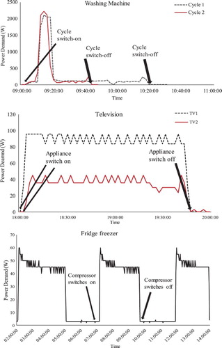
Switch-on events are identified when the power mode of the appliance changes from either off-mode (zero power demand) or stand-by mode (a low power demand) to on-mode. Through testing and visual inspection, the assumption was made that a switch-on event occurs when the appliance power demand changes from 3 W or lower to 6 W or higher. The monitoring equipment records power levels at 3 W intervals (DECC 2014a) and a reading of less than 3 W is taken as a reasonable assumption that an appliance is on standby mode or switched off. Switch-off events are identified in the opposite manner, when appliance power demand changes from 6 W or higher (on-mode) to 3 W or lower (off- or standby-mode). In the case of wet appliances, there were occasions of low power demands occurring mid-cycle which could be incorrectly identified as ‘switch-off events’; therefore, each use was manually inspected to ensure the correct switch-off times. Once the switch-on and switch-off events have been identified from the measured data, the three-appliance behaviour metrics are calculated for each appliance in the dataset.

4. The Household Appliance Usage Model

4.1. Overview

In this work, a stochastic model of the occupant behaviours of household appliance use is developed. The Household Appliance Usage Model (HAUM) is implemented as a MATLAB script. The HAUM simulates the occupants’ use of appliances within multiple homes over a chosen time period. The model works as follows:

• The buildings to be modelled and the appliances within each building are specified. For example, Household 1 with washing machine, dishwasher, cooker, etc., and Household 2 with washing machine, tumble dryer, grill, etc. In this work, 225 households with 176 washing machines, 18 washing-drying machines, etc., are specified which are identical to HES dataset as presented in Figure 1.

• A time period for the simulations is chosen. For example, 27 days for Household 1, 28 days for Household 2, etc.

• For each appliance, the model calculates the three-appliance behaviour metrics as follows:

  1. The number of switch-on events that occur for each day in the monitoring period

  2. The time of day when each of these switch-on events occur

  3. The duration of each occurrence of an appliance use following a switch-on event.

The HAUM uses pdfs and cumulative density functions (cdfs) to implement a stochastic modelling process. As a result, the model generates different final results each time it is run and thus running the model multiple time can give information on the distributions of each of the appliance behaviour metrics.

4.2. Modelling the appliance behaviour metrics

Figure 4 shows a schematic of the general modelling approach for calculating the appliance behaviour metrics within the HAUM. Three steps are shown in the figure. Step 1 shows a cdf which is constructed from the HES measurements (based on the results of calculating Metric 1 in Table 2) and is used to estimate the number of switch-on events which occur in a single day. The cdf can be calculated either as a cdf for each household with a particular appliance type (i.e. 176 cdfs representing each household with washing machines in the HES dataset) or it can be the cdf based on an average household (i.e. one cdf based on averaging 176 households with washing machines in the HES dataset). In Figure 4, an example is given for a cdf of number of switch-on events of a washing machine. Step 2 shows a pdf which is constructed from the HES measurements (Metric 2) and is used to estimate the time of day when a switch-on event occurs. Again this can be calculated either for an individual household or as an average for all households with a particular appliance type. In Figure 4, an example is given for pdf of switch-on times of washing machine. Each time step of a day is associated with a value between 0 and 1 corresponding to the probability of switching that appliance on at that time of day. For each time step the switch-on probability would be the sum of measured ‘switches on’ observed divided by the total number of days. Step 3 shows another cdf which is constructed from the HES measurements (Metric 3) and is used to estimate the duration of an appliance use. This can be calculated either as an average of all appliances or for an individual appliance.

Figure 4. Schematic of modelling the appliance behaviour metrics in the HAUM model.

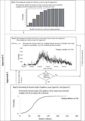
Two approaches to modelling the appliance behaviour metrics are tested in this paper. Approach 1 takes a simple approach often used in appliance behaviour modelling where the metrics are calculated using only Step 2 and Step 3. In Step 2, switch-on events are determined by ‘stepping through’ the day in 2-minutely time steps. For the first time step, a uniform random number is generated and the appliance is switched on if the generated value is smaller than or equal to the probability given by the pdf at that time step. If a switch-on event does not occur, then the process steps to the next 2-minute time step and the test for a switch-on event is repeated. If a switch-on event does occurs, then the duration of the appliance use is calculated using Step 3. A second uniform random number is generated and is used to calculate the duration by reading the duration in the cdf of Step 3 which corresponds to cumulative probability given by the random number. Inverse transform sampling is used to derive the duration of the appliance run from the developed cdfs in Step 3. In the inverse transform algorithm, uniform random deviates are sampled (i.e. random numbers between 0 and 1) and each random number is compared against the table of cdfs in Step 3. The first outcome for which the random deviate is smaller than (or is equal to) the associated cumulative probability corresponds to the sampled outcome. Once the appliance run has completed, Step 2 continues at the next time step following the end of the appliance run. Approach 2 takes a different approach designed to improve the modelling of the number of switch-on events (i.e. Metric 1) and uses Steps 1, 2 and 3 in its calculations. Step 1 is used to calculate the number of switch-on events which occur in each day. Inverse transform sampling is used to derive the number of switch-on events from the developed cdfs in Step 1. Once this is completed, Step 2 is used to calculate the time of day when each of the switch-on events occur; the ‘stepping through’ the pdf is run until the model gives the number of switch-on times determined by the cdf. Step 3 is used to estimate the durations in a similar manner to Approach 1.

5. Description of the HAUM variants used in this work

Table 3 shows the different variations of the HAUM which are used to generate the results in this paper. Two approaches are used, Approach 1 (Steps 2 and 3 in Figure 4) and Approach 2 (Steps 1, 2 and 3 in Figure 4). For each approach, three variants are tested based on the method of constructing the pdf for Step 2 and cdfs for Steps 1 and 3. Model variants starting with ‘AvgHs’ use the average household cdfs and pdfs for the calculations, whereas ‘IndHs’ denotes the use of an individual household cdf and pdf. The individual household cdf and pdf are assigned to the building at the start of the modelling session and remains constant through the simulation. Model variants ending with ‘AvgApp’ use an average appliance cdf to calculate durations and with ‘IndApp’ use individual appliance cdfs. The average (Avg) indicates the pdfs and cdfs were developed as a single pdf or cdf representing an average of all households or appliances, whereas individual (Ind) was developed for each household/appliance, resulting in several pdfs and cdfs (176 washing machine duration cdfs or 105 cooker switch-on pdfs). These model variants were developed in order to test the effect of averaging the data on representing the diversity in occupant behaviour.

Table 3. HAU model variants for two main approaches described with their methods.

		Calculation method for:
Approach type	Variant	Metric 1: Number of switch-on events	Metric 2: Switch-on time of day	Metric 3: Duration
Approach 1	AvgHs_AvgApp	Calculated using Step 2		Calculated using Step 3
		pdf based on an average household		cdf based on an average appliance
	AvgHs_IndApp	Calculated using Step 2 pdf based on an average household		Calculated using Step 3 cdf based on an individual appliance
	AvgHs_IndApp	Calculated using Step 2		Calculated using Step 3
		pdf based on an individual household		cdf based on an average appliance
Approach 2	AvgHs_AvgApp	Calculated using Step 1	Calculated using Step 2	Calculated using Step 3
		cdf based on an average household	pdf based on an average household	cdf based on an average appliance
	AvgHs_IndApp	Calculated using Step 1	Calculated using Step 2	Calculated using Step 3
	AvgHs_IndApp	cdf based on an average household	pdf based on an individual household	cdf based on an individual appliance
	IndHs_AvgApp	Calculated using Step 1	Calculated using Step 2	Calculated using Step 3
	AvgHs_IndApp	cdf based on an average household	pdf based on an individual household	cdf based on an individual appliance

The model is developed for 16 appliance types. One-way ANOVA test was conducted to compare the effect of household type, occupant number and day types on the mean of average daily number of switch-on events, switch-on times and duration. For several appliances, ANOVA is not performed as it violates one of the assumptions of ANOVA homogeneity of variances. Some of the appliances have too small sample sizes. For the rest of the appliances, the ANOVA test results show that there is no significant effect of these characteristics on the average daily number of switch-on events. Therefore, there is no sub-population for household types, and no occupant number or day types are considered. Two hundred and twenty-five households have generated exactly the same with monitoring period in Figure 2 by applying the HAUM procedure (e.g. 176 households with washing machines for 27 days; 84 households with tumble dryer for 28 days, etc.). Each variant is run 100 times to generate the results in Section 6.2. The simulation results are shown by taking the average values of 100 simulation runs. The ability of the HAUM to recreate the patterns observed in the monitored dataset is compared. Therefore, the monitored data are not divided into training and test sets in order to prevent the bias when comparing the approaches.

6. Results

6.1. Identifying and quantifying the appliance behaviour metrics in the HES dataset

6.1.1. Metric 1: Number of switch-on events

For each appliance in the HES dataset, the number of switch-on events (Metric 1) per day is calculated using the approach given in Section 3.2. Table 4 shows the summary statistics for the results of Metric 1 for the 225 homes in the HES dataset. For appliance categories, cold appliances have the highest average daily number of switch-on events, a mean of 28.5 switch-on times per day based on the 332 cold appliances in the dataset. Wet appliances have the lowest average daily number of switch-on events with a mean of 0.75. Chest freezers are the appliance types that have the highest average daily number of switch-on events with a mean of 42.6 switch-on times per day based on the 34 chest freezers in the dataset. The results highlight the variation in average daily number of switch-on events for all appliance types. For example, the results show that one chest freezer has an average of 109.7 switch-on events per day throughout its monitoring period (the highest observed in the dataset for televisions) and another had an average of 5.5 (the lowest observed). Similarly, one TV 1 has an average of 5.8 switch-on events per day throughout its monitoring period (the highest observed in the dataset for chest freezers) and another had an average of 0.04 (the lowest observed). Grills have the lowest number of daily switch-on times, a mean of 0.24 switch-on times per day based on the five grills in the dataset. The results show that the larger sample size, the smaller the confidence interval is. For example, washing machines (n = 176) has a mean of 0.78 switch-on times per day with ± 0.08 (95% confidence interval), whereas the washing-drying machines (n = 18) has a mean of 1.03 switch-on times per day with ± 0.46 (95% confidence interval). This indicates the importance of high sample size for estimating the switch-on statistics.

Table 4. Statistics for average daily number of switch-on events for each appliance type as recorded in the 225 homes in the HES dataset.

Appliances			Average daily number of switch-on events for each appliance type over the monitoring period^a
Appliance category	Appliance types	n	Mean^b	95% C.I^c of the mean	Minimum	Maximum	Median
Wet appliances	Washing machine	176	0.78	±0.08	0.04	3.5	0.6
	Washing-drying machine	18	1.03	±0.46	0.10	3.8	0.8
	Tumble dryer	84	0.71	±0.13	0.04	3.4	0.6
	Dishwasher	86	0.65	±0.07	0.10	3.8	0.6
	All	364	0.75	±0.06	0.04	3.8	0.6
Cooking appliances	Cooker	105	2.09	±0.39	0.04	9.8	1.5
	Oven	44	0.98	±0.33	0.04	5.6	1.3
	Hob	9	1.35	±0.44	0.50	2.5	0.3
	Grill	5	0.24	±0.10	0.07	0.4	0.7
	All	163	1.74	±0.30	0.04	9.8	1.1
Televisions	TV1	81	2.20	±0.24	0.04	5.8	1.9
	TV2	41	1.56	±0.35	0.04	5.0	1.7
	TV3	20	0.94	±0.45	0.04	3.4	0.5
	All	142	1.84	±0.20	0.04	5.8	1.8
Electric shower		73	1.02	±0.16	0.04	1.5	1.0
Cold appliances	Fridge	89	22.2	±3.50	2.80	85.4	17.6
	Fridge freezer	129	27.7	±3.30	2.90	125.3	24.0
	Chest freezer	34	42.6	±9.80	5.50	109.7	36.0
	Upright freezer	81	29.4	±3.50	4.40	95.9	25.9
	All	332	28.5	±2.13	2.80	125.3	36.5

^aAverage daily number of switch-on events is calculated as the average (mean) of the number of switch-on events for each day over the monitoring period. For example, if an appliance is monitored for 30 days, then the average daily number of switch-on events is the mean of 30 values, where the 30 values are the number of switch-on events that occur on each of the 30 days.

^bThis ‘mean’ refers to the mean of the average daily number of switch-on events for each appliance type. For example, in the case of washing machines this is calculated as the mean of 176 values, where each value is the average daily number of switch-on events for one washing machine. The other statistics in this table are calculated in a similar manner.

^cThis refers to the 95% confidence interval of the mean.

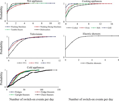
The cdfs of number of switch-on events per day for the 16 appliance types are shown in Figure 5. These were used to determine the switch-on events in Step 1 of Approach 2 (Section 4.2). The results show the variation in daily number of switch-on events observed for all appliance types in the HES dataset with some days recording no use of appliance (0 switch-on events) and other days recording many switch-on events. For example, grills were not used at all for 80% of the days observed (least used) whereas cold appliances had at least one number of switch-on events per day The cold appliances have the highest number of switch-on events and one chest freezers had 144 switch-events in a single day. This is caused by the constant cycling of the chest freezers as the compressor switches on and off throughout the day.

Figure 5 Cumulative distribution of duration length per usage of appliance types of the appliance category (wet appliances, cooking appliances, televisions, electric showers and cold appliances).

6.1.2. Metric 2: Switch-on times of a day

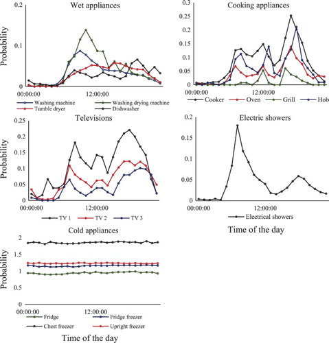
Figure 6 shows the frequency of mean hourly switch on times varying over daily profiles for the 16 appliance types. These profiles are calculated using the definition given at Section 4.2 and shown in here for hourly time slots in order to demonstrate the overall trend of the profiles. However, for the modelling, two-minutely probabilities of switch-on times were used. The results highlight the differences that occur in switch-on times across appliance categories and appliance types and show that different appliances are used at different times of the day. Cooking appliances are switched on around morning, noon and evening times which are presumably meal times. Peak time occurs in the evening for dishwashers after the evening meal, whereas the peak time for washing machines is observed in the morning. Cold appliances are switched on repeatedly throughout the day. Televisions are switched on starting from the early morning and peak times occur both in the morning and in the evening.

Figure 6. Average hourly number of switch-on events (y-axis) vs. time of day (x-axis) for each appliance type as recorded in the 225 homes in the HEUS dataset.

6.1.3. Metric 3: Duration (run time of appliances)

For each appliance in the HES dataset, duration of appliance use (Metric 3) per usage was calculated using the approach given in Section 3.2. Table 5 shows the summary statistics for Metric 3 for the 225 homes in the HES dataset. ‘Television 1’ had the longest duration per usage, a mean of 160.2 minutes based on the 81 ‘Television 1’ appliances in the dataset. The next longest are ‘Television 3’ (129.8 minutes) and ‘Television 2’ (119.7). Electric showers have the shortest duration per usage, a mean of 9.44 minutes based on the 73 electric showers in the dataset. After TVs, wet appliances are the appliance category with the second highest duration of appliance use, a mean of 75.8 minutes per usage in total based on the 364 wet appliances in the dataset. The results show that one electric shower has an average of 25.5 minutes of duration per usage throughout its monitoring period (the highest observed in the dataset for electric showers) and another had an average of 2.0 (the lowest observed).

Table 5. Statistics for average duration length per usage monitoring period (minutes) and duration length per usage (minutes) for each appliance over the monitoring period.

Appliances			Average duration length per usage for each appliance over the monitoring period (minutes)
Category	Types	n	Mean	95% CI of the mean (95%)	Minimum	Maximum	Median
Wet appliances	Washing machine	176	75.7	±3.4	27.7	172.4	72.6
	Washing-drying machine	18	86.8	±28.0	53.0	211.6	73.0
	Tumble dryer	84	70.4	±12.8	21.0	165.2	65.0
	Dishwasher	86	79.2	±13.4	28.1	136.5	80.5
	All	364	75.8	±2.70	21.0	211.6	73.8
Cooking appliances	Cooker	105	40.7	±8.00	6.4	128.5	34.4
	Oven	44	47.0	±24.0	14.0	134.0	44.5
	Hob	9	37.5	±37.1	13.5	102.2	29.1
	Grill	5	11.9	±5.0	9.2	13.4	12.3
	All	163	39.6	±3.97	6.4	134.0	36.0
Televisions	TV1	81	160.2	±35.0	7.9	654.7	100.0
	TV2	41	119.7	±23.3	4.0	444.8	82.6
	TV3	21	129.8	±29.6	38.3	465.8	123.8
	All	143	134.4	±18.8	4.0	654.7	98.7
Electric showers		73	9.44	±0.95	2.0	25.5	8.7
Cold appliances	Fridge	88	36.6	±34.0	3.6	744.7	18.4
	Fridge freezer	129	38.4	±38.0	8.0	473.7	23.4
	Chest freezer	34	29.3	±28.9	5.5	206.1	14.7
	Upright freezer	81	27.8	±26.8	8.7	171.5	22.7
	All	334	36.6	±6.4	3.6	744.7	22.0

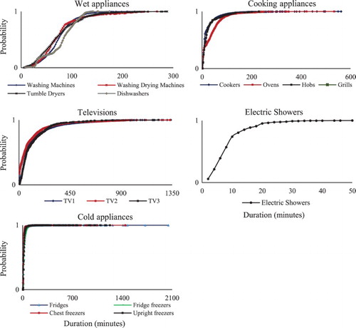
The cumulative distribution functions of the duration per usage for the 16 appliance types are shown in Figure 7. The graphs show that there is a great variation in the duration lengths of individual appliance usages in the HES dataset. Electric showers have low duration lengths, ranging between 2 and 50 minutes. One ‘Television 1’ was switched on for 22.5 hours in a single day (the highest observed in the dataset for televisions). The variation in duration is high for cold appliances and the compressors appear to be on for a long time, in one case, for over 34 hours. Durations per usage of wet appliances are less than 300 minutes with 80% of the durations less than 100 minutes. The duration length of washing machines varied from 10 to 244 minutes.

Figure 7. Cumulative distribution of duration length per usage for 16 appliance types.

6.2. Simulation results

6.2.1. Comparison of the number of switch-on events

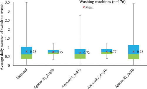
First, the results of the simulations for washing machine appliances are presented. Simulations are run for four model variants: Approach1_AvgHs, Approach1_IndHs, Approach2_AvgHs and Approach2_IndHs) as set out in Section 5. Here the average appliance pdf is used to calculate appliance durations as this section is focusing on the Approach1/Approach2 and AvgHs/IndHs comparisons. Each model variant is simulated 100 times and Figure 8 shows the distribution of the 100 simulation results for each of the model variants. It is clear that, on average, Approach1 underestimates the number of switch-on events per day compared to the measured data (0.78 switch-on events per day). Approach1 predicts, on average, 0.73 switch-on events per day for an average household pdf and 0.70 for an individual household pdf. Approach2 predicts the number of switch-on events close to the measured data result, with both the average and individual household pdf results as 0.78. This is an important result as Approach1 is the approach taken by many past studies and the reasons why Approach1 is under-predicting is discussed in Section 7.2. As expected, using individual household pdfs or cdfs rather than average household results in greater variation in the simulation runs. This increased variation occurs because, for each of the 100 simulation runs, the same cdf is used for the AvgHs results whereas many different possible combinations of cdfs are used for the IndHs results.

Figure 8 Boxplots of the mean of average daily number of switch-on events of washing machines resulting from 100 simulation runs. Approach 1 uses a single-day pdf (Step 2) and Approach 2 uses a cfd (Step 1) to estimate the number of switch-on events per day. AvgHS is an ‘average household’ and IndHs is an ‘individual household’.

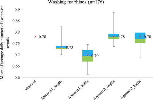
Table 6 shows that the findings seen in Figure 8 for washing machines are observed for all appliance types in the dataset. In Table 7, the measured, Approach1_AvgHs, Appraoch1_IndHs, Approach2_AvgHs and Approach2_IndHs results are shown for the mean average daily number of switch-on events, based on 100 simulation runs for each appliance type. The percentage difference of the mean value of simulation from the measured dataset is indicated in parenthesis. As can be seen from Table 7, mean is underestimated by Approach 1 regardless of the HAUM variant. However, IndHs predicted the average daily number of switch-on events even less than AvgHs in Approach 1 (up to −16%) for all appliances. Approach 2 predicted the average daily number of switch-on events correctly for all appliances regardless of the model variant.

Table 6. Statistics of the average daily number of switch-on events for 16 appliances of averaged from 100 simulation runs of Approach 1 and Approach 2 with model variants AvgHs_AvgApp and IndHs_AvgApp and measured value.

			Mean of average daily number of switch-on events for each appliance type
				Approach 1		Approach 2
Appliance category	Appliance types	n	Measured	AvgHs	IndHs	AvgHs	IndHs
Wet appliances	Washing machine	176	0.78	0.73 (−6%)	0.70 (−11%)	0.78 (0%)	0.78 (0%)
	Washing-drying machine	18	1.03	0.96 (−8%)	0.89 (−15%)	1.03 (0%)	1.03 (0%)
	Tumble dryer	84	0.71	0.67 (−5%)	0.64 (−9%)	0.71 (0%)	0.71 (0%)
	Dishwasher	86	0.65	0.62 (−5%)	0.59 (−9%)	0.65 (0%)	0.65 (0%)
	All	364	0.75	0.71 (−5%)	0.68 (−10%)	0.75 (0%)	0.75 (0%)
Cooking appliances	Cooker	105	2.09	2.03 (−5%)	1.83 (−9%)	2.09 (0%)	2.09 (0%)
	Oven	44	0.98	0.95 (−5%)	0.87 (−9%)	0.98 (0%)	0.98 (0%)
	Hob	9	1.35	1.28 (−5%)	1.26 (−7%)	1.35 (0%)	1.35 (0%)
	Grill	5	0.24	0.24 (−4%)	0.23 (−1%)	0.24 (0%)	0.24 (0%)
	All	163	1.74	1.65 (−5%)	1.62 (−8%)	1.74 (0%)	1.74 (0%)
Televisions	TV1	81	2.20	2.07 (−6%)	1.99 (−9%)	2.20 (0%)	2.20 (0%)
	TV2	41	1.56	1.34 (−14%)	1.23 (−21%)	1.56 (0%)	1.56 (0%)
	TV3	21	0.94	0.87 (−7%)	0.81 (−14%)	0.94 (0%)	0.94 (0%)
	All	143	1.84	1.64 (−11%)	1.51 (−18%)	1.84 (0%)	1.84 (0%)
Electric shower		73	1.02	1.00 (−2%)	0.95 (−7%)	1.02 (0%)	1.02 (0%)
Cold appliances	Fridge	88	22.2	19.02 (−4%)	17.74 (−20%)	22.2 (0%)	22.2 (0%)
	Fridge freezer	129	27.7	23.30 (−16%)	21.81 (−21%)	27.7 (0%)	27.7 (0%)
	Chest freezer	34	42.6	36.11 (−15%)	33.01 (−23%)	42.6 (0%)	42.6 (0%)
	Upright freezer	81	29.4	25.18 (−14%)	23.02 (−22%)	29.4 (0%)	29.4 (0%)
	All	334	28.5	24.23 (−15%)	22.23 (−22%)	28.5 (0%)	28.5 (0%)

Table 7. Comparison of the mean of the duration length (minutes) of appliance usage for 16 appliances of the 100 simulations of model variants AvgHs_AvgApp and IndHs_AvgApp.

			Mean of average duration length per usage for each appliance type
				Approach 1		Approach 2
Appliance category	Appliance types	n	Measured	AvgApp	IndApp	AvgApp	IndApp
Wet appliances	Washing machine	176	75.7	76.7 (1%)	76.4 (0%)	75.6 (0%)	75.73 (0%)
	Washing-drying machine	18	86.8	86.9 (0%)	85.5 (−1%)	86.7 (0%)	86.83 (0%)
	Tumble dryer	84	70.4	71.8 (2%)	70.2 (0%)	70.3 (0%)	70.2 (0%)
	Dishwasher	86	79.2	81.1 (2%)	81.0 (2%)	79.1 (0%)	79.23 (0%)
	All	364	75.8	77.3 (0%)	75.3 (0%)	75.8 (0%)	75.8 (0%)
Cooking appliances	Cooker	105	40.7	39.5 (−3%)	40.3 (1%)	40.68 (0%)	40.59 (0%)
	Oven	44	47.0	46.1 (2%)	46.5 (0%)	46.9 (0%)	46.81 (0%)
	Hob	9	37.5	36.8 (−2%)	37.4 (0%)	37.5 (0%)	37.39 (0%)
	Grill	5	11.9	11.6 (0%)	12.0 (1%)	11.9 (0%)	11.79 (0%)
	All	163	39.6	39.2 (−1%)	39.3 (0%)	39.6 (0%)	39.3 (0%)
Televisions	TV1	81	160.2	161.9 (1%)	161.3 (1%)	160.3 (0%)	160.18 (0%)
	TV2	41	119.7	120.1 (0%)	120.0 (0%)	119.8 (0%)	119.68 (0%)
	TV3	21	129.8	130.8 (1%)	129.2 (0%)	129.9 (0%)	129.78 (0%)
	All	143	134.4	134.6 (1%)	134.4 (0%)	134.4 (0%)	134.5 (0%)
Electric shower		73	9.4	9.4 (0%)	9.4 (0%)	9.3 (−1%)	9.4 (0%)
Cold appliances	Fridge	88	36.6	36.6 (0%)	36.6 (0%)	36.6 (0%)	36.6 (0%)
	Fridge freezer	129	38.4	38.7 (0%)	38.4 (0%)	38.7 (0%)	38.4 (0%)
	Chest freezer	34	29.3	29.7 (0%)	29.3 (0%)	29.7 (0%)	29.3 (0%)
	Upright freezer	81	27.8	27.7 (0%)	27.8 (0%)	27.7 (0%)	27.8 (0%)
	All	334	36.6	36.8 (0%)	36.5 (0%)	36.6 (0%)	36.6 (0%)

It is also important to test that the simulation process predicts a reasonable variation in the switch-on events of the appliances across households. Figure 9 shows the distribution (boxplots) of the values of average daily number of switch-on events of washing machines resulting from one simulation run (176 washing machines simulated once) with the measured values. The HAU variants’ ability to capture the variability of the average daily number of switch-on events is tested depending on how the switch-on pdfs are developed (AvgHs vs. IndHs). Results show that IndHs_AvgApp is better at capturing the variation of daily average number of switch-on events as opposed to AvgHs_AvgApp. The interquartile range (the difference between the 25th quantile and 75th quantile) is calculated for each HAU model variant to indicate the variability around the median; the interquartile range is reduced from 0.64 to 0.25 by 61% for AvgHs_AvgApp whereas for IndHs_AvgApp it is increased from 0.64 to 0.75 by 18%. The range of mean of average daily number of switch-on times (difference between maximum and the minimum values) is reduced from 3.48 to 0.86 (by 75%) and from to 3.48 to 3.42 (by 2%) for AvgHs_AvgApp and IndHs_AvgApp, respectively.

Figure 9. Boxplots of the average daily number of switch-on events of washing machines resulting from one simulation compared with the measured average daily number of switch-on events (176 washing machines).

6.2.2. Comparison of switch-on times profiles

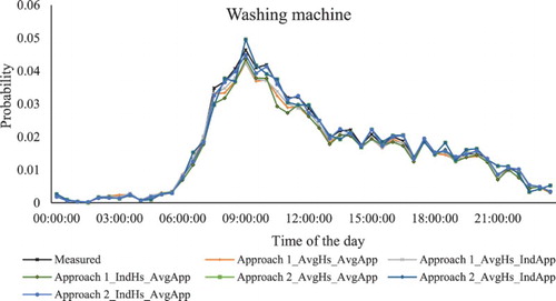
Half hourly (30 minutes) probabilities of switching on for the 100 simulated values of HAU model variants are compared with measurements, for washing machines, in Figure 9. All model variants of the two main approaches of the HAU model do comparatively well in predicting the half hourly probability switch-on times over the day. However, as Approach 1 predicts a lower mean of the number of switch-on events (Table 7), there is a gap between the lines even though the shape of the daily profile (the time of the peak values, etc.) is predicted well (Figure 10).

Figure 10. Comparison of the half-hourly (30 minutes) probability of switching on of measured and 100 simulated households of washing machines.

6.2.3. Comparison of duration distributions

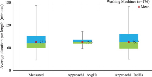
The results of the simulations for mean value of the average duration length per usage for each appliance type are presented in Table 7. Simulations were run for four model variants: Approach1_AvgHs, Approach1_IndHs, Approach2_AvgHs and Approach2_IndHs (as defined in Section 5). Each model variant is simulated 100 times. As expected, since both approaches use the same method (using step 3) to predict the duration for each usage, there was not a difference in the values of average duration length per usage for each appliance over the monitoring period between Approach 1 and Approach 2 regardless of the model variant. Both modelling approaches predicted the average duration length per usage correctly.

It is also important to test that the simulation process predicts a reasonable variation in the duration length per usage of the appliances across households. Figure 11 shows the distribution (boxplots) of the values of duration length for each usage of washing machines resulting from one simulation run (176 washing machines simulated once) of AvgHs_AvgApp and AvgHs_IndApp of Approach 2 with the measured values. Results show that AvgHs_IndApp is better at capturing the variation of daily average number of switch-on events as opposed to AvgHs_AvgApp. The interquartile range (the difference between the 25^th quantile and 75^th quantile) is calculated for each HAU model variant to indicate the variability around the median; the interquartile range is reduced from 30.8 to 9.6 by 69% for AvgHs_AvgApp whereas for AvgHs_IndApp it is increased from 30.8 to 35.7 by 16%. The range of mean of average daily number of switch-on times (difference between maximum and the minimum value) is reduced from 144.7 to 42.1 (by 75%) and from to 144.7 to 139.2 (by 4%) for AvgHs_AvgApp and AvgHs_IndApp, respectively.

Figure 11. Boxplots of the average duration length per usage of washing machines resulting from one simulation compared with the measured average duration length (176 washing machines).

7. Discussion

7.1. Occupant behaviour monitoring and data collection methodologies

This study has contributed to an improved understanding of how to model the occupant behaviour of household appliance use in UK homes. The results obtained are however limited by the relatively short monitoring period and small sample size. For instance, the homes were monitored for between 20 and 45 days, with an average monitoring period of 27.7 days, after which the equipment was moved to another household. This was done to minimize the monitoring equipment costs of the survey. As a result, different households with different appliances were monitored in different seasons throughout the monitoring period. This makes it difficult to discern if the variations in the appliance occupant behaviour is due to household characteristics, seasonal changes or other factors. As smart and connected homes make monitoring easier and less costly, future surveys could have greater sample sizes and monitor homes in parallel, and for longer time periods. Such longitudinal studies will allow the complex interaction of factors which lead to different behaviours in different household types at different times of year to be better understood.

Attempts were made to differentiate the occupant behaviours based on the number of people living in the home and the household type (i.e. family vs. single person, working household vs. pensioner), controlling for other characteristics. However, the HES dataset proved to be too small to perform meaningful statistical comparisons in this case. Splitting the sample into subgroups may also degrade the model’s predictive performance due to data scarcity. To give examples of the small subgroups: there were only five grills observed in the dataset, only five households with four occupants and only three households with five occupants. A much larger future study would be beneficial to improve the representativeness of the survey and to validate the findings of the existing study.

Furthermore, the HES study recorded the power demands of the appliances rather than the actions of individual occupants, and it was necessary to infer the occupant behaviour from these measurements. Occupant behaviour had to be defined at the household level rather than at the individual level as it was only possible to track when appliances are switched on, not by whom. Appliance usage patterns by an individual may be inter-correlated and it is not clear from the current analysis if it is possible to generalize this to other appliance correlations as it is not known the order of appliance use by an individual occupant.

7.2. Appliance behaviour modelling and simulation methodologies

Occupant behaviour modelling of household appliance use is still a relatively new field of research and there is more work needed to improve our knowledge of the suitability of the numerous modelling approaches currently available. A strength of this study, as opposed to previous studies which have relied on diary-based ‘time of use’ datasets, is the use of monitored electrical power demands of individual appliances to develop the high-resolution stochastic model. The strength of the HAUM is that it considers multiple stochastic factors within the households: appliance switch-on time probabilities and usage durations developed for individual homes. For example, only inter-household variation (variation among different household groups) could be considered for past models that have been developed using TOU datasets based on one-day diaries (Tanimoto, Hagishima, and Sagara 2008; Richardson et al. 2010; Widén, Molin, and Ellegård 2012; Wilké et al. 2013).

These models averaged the one-day profiles for different sub-population to integrate the variation among households. The results of this paper show that averaging profiles (AvgHs. and AvgApp.) for a population underestimates the variation. This was shown in the box plots in Figures 9 and 11 that averaging the data (AvgHs and AvgApp) similar to Wilké et al. (2013) and Richardson et al. (2010) underestimates the diversity. As a result, the corresponding uncertainty of building performance simulation predictions may be greatly underestimated. This limits one of the major benefits of stochastic occupant behaviour modelling. Moreover, not addressed in this paper, but worthy of future research, occupant behaviour diversity may be advantageous with regards to instantaneous electricity demand since certain systems must be sized to meet the maximum expected simultaneous load or may underestimate the problem of grid instability (Baetens et al. 2010).

The switch-on times of appliances are predicted based on relative time-of-day use potential. This study found that the method which predicted the time when a switch-on event occurs using pdfs (Approach 1 and Approach 2) gave good results in the case of switch-on times over one day, in agreement with studies in literature which performed similar validation (Page 2007; Wilké et al. 2013). The HAUM has proven itself capable of simulating the switch-on times over a day. However, the Approach 1 method of assigning switch-on times based on switch-on pdfs and followed by assigning durations from cdfs is problematic because the average daily number of switch on times is under-predicted (Table 7). This result may arise because of the process of stepping through the time steps in time order and effectively jumping over a number of time steps when a switch-on event occurs and a duration is assigned, reducing the number of times that the pdf is used to test for a switch-on event. This effect is more pronounced in model variant IndHs as the probabilities are more ‘peaky’ and occur at similar times of the day (due to habits of the households), causing the reduction at the mean values up to 12% (Table 7). However, Approach 2 appears to solve this problem and predicts similar numbers of switch-on event compared to the measured data. The simulation results shown in Table 7 and Figures 9 and 11 support the argument that models developed on individual home profiles (IndHs and IndApp) capture the variation (both switch-on probabilities and appliance usage duration) much better than averaged profiles (AvgHs and AvgInd) regardless of whether Approach 1 or Approach 2 is used. This is partly explained by the fact that when a single ‘average’ cdf is created from the dataset, durations are selected mostly around the median thereby hindering the variation in durations for individual usages; whereas for AvgHs_IndApp, the per-appliance cdfs are more diverse resulting in a wider range of values.

For cold appliances, off-sequence durations (when the compressor is not on) have not been discussed in this study. Although Approach 2 predicts the number of times when the compressor switches on, it has no constraint for the off-durations; therefore, the sequences might be quite uneven. A future approach might be to determine an on-sequence profile from cdfs of on-durations and, once the on-sequence ends, the duration of the off-sequence could be deduced from an equivalent off-sequence duration profile.

8. Conclusions

This paper introduces a high-resolution stochastic HAUM based on electrical power demand measurements gathered from 225 homes in the UK as part of the UK Government’s HES. Sixteen appliance types were selected from the dataset for analysis and modelling. The appliances were modelled by defining probabilities for the number of switch-on events, the switch-on time and the duration of appliance usage.

The conclusions arising from this study are:

• -The HES dataset shows that there is a significant variation between households in the number of appliance switch-on events (Table 4). For example, cold appliances are switch-on between an average of 2.8 times per day in one household and an average of 125.3 times in another household.

• -There is also significant variation in number of switch-on events across days (Figure 5). Daily appliance use ranges from zero between 8 times per day for electric showers and one between 150 times per day for cold appliances.

• -There is a further variation in the switch-on times of appliances across different days and households for all 16 appliance types (Figure 6). Cooking appliances are switched on around morning, noon and evening times (presumably meal times). Peak time occurs in the evening for dishwashers after the evening meal, whereas the peak time for washing machines is observed in the morning. Cold appliances are switched on repeatedly throughout the day.

• -The length of time that appliances are used is also highly variable (Table 5) and average household appliance durations vary significantly. For example, in the case of electric showers duration lengths vary from an average of 2 minutes for one household to an average of 25.5 minutes for another household. Individual appliance use durations also vary (Figure 7). For electric showers, the duration ranges from 2 minutes up to 50 minutes. This is the effect of the occupants’ preference for using the appliances for different durations and of those appliances, such as wet appliances, which have different durations due to choice of programmes.

• -The modelling approach (Approach 2) that first assigns the daily number of switch-on events, and then determines the time of the switch-on events by ‘stepping through’ the pdf and durations from cdfs, predicts the average daily number of switch-on events well (less than 0.1% difference) (Table 6). Approach 1 (similar to previous studies) does not first assign the daily number of events and simply determines the number of switch-on events and switch-on times by ‘stepping through’ the pdf and durations from cdfs. Approach 1 was shown to significantly underestimate the average daily number of switch-on events.

• -The model variants that use individual household switch-on pdfs and individual appliance duration cdfs simulated variation in average daily number of switch-on times and durations better than those model variants developed based on averaged households and averaged appliances (Figures 9 and 11).

Modelling the use of appliances is a challenging task, given the diversity of appliances available and the variability in occupant behaviour from one household to another household. Averaging the data for developing the metrics is shown to suppress the diversity of the predicted occupant behaviour within the individual households. This limitation is often ignored by modellers that use TOU surveys, based on diaries recorded in a single day, to develop their models. However, the results here show that variation within the individual households is an important factor and the choice of modelling approach can play a significant role in predicting the occupant behaviour of appliance usage. In future work, the current study will be extended to include a comparison of electricity demand profiles of households to investigate the effect of demand side management on the overall household electricity profiles.

Acknowledgements

Household Electricity Survey data acquisition was coordinated by the Department of Energy and Climate Change of United Kingdom. These data can be downloaded by sending an e-mail to [email protected].

Additional information

Funding

This research was made possible by Engineering and Physical Sciences Research Council (EPSRC) support for the London-Loughborough Centre for Doctoral Research in Energy Demand [grant number EP/H009612/1].

References

- Abushakra, B., and D. E. Claidge. 2001. “Accounting for the Occupancy Variable in Inverse Building Energy Baselining Models.” Paper presented at the International Conference for Enhanced Building Operation (ICEBO), Austin, TX, July.
- Baetens, R., R. De Coninck, L. Helsen, and D. Saelens. 2010. “The Impact of Load Profile on the Grid-interaction of Building Integrated Photovoltaic (BIPV) Systems in Low-energy Dwellings.” Journal of Green Building 5 (4): 137–147. doi: 10.3992/jgb.5.4.137
- Capasso, A., W. Grattier, R. Lamedica, and A. Prudenzi. 1994. “A Bottom-up Approach to Residential Load Modelling.” IEEE Transactions on Power Systems 9 (2): 957–964. doi: 10.1109/59.317650
- Cogan, D., M. Camilleri, N. Isaacs, and L. French. 2006. “National Database of Household Appliances – Understanding Baseload and Standby Power Use.” Paper presented at the Energy Efficiency in Domestic Appliances and Lighting (EEDAL) Conference, London, June.
- DECC. 2014a. “Household Electricity Survey.” Department of Energy and Climate Change. Report available from: https://www.gov.uk/government/publications/household-electricity-survey--2
- DECC. 2014b. “Energy Follow-up Survey (EFUS): 2011.” Department of Energy and Climate Change. Report available from: https://www.gov.uk/government/statistics/energy-follow-up-survey-efus-2011
- D’Oca, S., and T. Hong. 2014. “A Data-mining Approach to Discover Patterns of Window Opening and Closing Behavior in Office.” Building and Environment 82: 726–739. doi: 10.1016/j.buildenv.2014.10.021
- Feng, X., D. Yan, and T. Hong. 2015. “Simulation of Occupancy in Buildings.” Energy and Buildings 87: 348–359. doi: 10.1016/j.enbuild.2014.11.067
- Firth, S. K., K. Lomas, A. Wright, and R. Wall. 2008. “Identifying Trends in the Use of Domestic Appliances from Household Electricity Consumption Measurements.” Energy and Buildings 40 (5): 926–936. doi: 10.1016/j.enbuild.2007.07.005
- Grandjean, A., J. Adnot, and G. Binet. 2012. “A Review and an Analysis of the Residential Electric Load Curve Models.” Renewable and Sustainable Energy Reviews 16 (9): 6539–6565. doi: 10.1016/j.rser.2012.08.013
- Guerra Santin, O., L. Itard, and H. Visscher. 2009. “The Effect of Occupancy and Building Characteristics on Energy Use for Space and Water Heating in Dutch Residential Stock.” Energy and Buildings 41 (11): 1223–1232. doi: 10.1016/j.enbuild.2009.07.002
- Haldi, F., and D. Robinson. 2010. “Adaptive Actions on Shading Devices in Response to Local Visual Stimuli.” Journal of Building Performance Simulation 3 (2): 135–153. doi: 10.1080/19401490903580759
- Hoes, P., J. L. M. Hensen, M. G. L. C. Loomans, B. de Vries, and D. Bourgeois. 2009. “User Behavior in Whole Building Simulation.” Energy and Buildings 41 (3): 295–302. doi: 10.1016/j.enbuild.2008.09.008
- Isaksson, C., and F. Karlsson. 2006. “Indoor Climate in Low-energy Houses – An Interdisciplinary Investigation.” Building and Environment 41 (12): 1678–1690. doi: 10.1016/j.buildenv.2005.06.022
- Paatero, J. V., and P. D. Lund. 2006. “A Model for Generating Household Electricity Load Profiles.” International Journal of Energy Research 30 (5): 273–290. doi: 10.1002/er.1136
- Page, Jessen. 2007. “Simulating Occupant Presence and Behaviour in Buildings.” PhD diss., École Polytechnique de Fédérale Lausanne.
- Reinhart, C. F., J. Mardaljevic, and Z. Rogers. 2006. “Dynamic Daylight Performance Metrics for Sustainable Building Design.” Leukos 3 (1): 1–25.
- Richardson, I., M. Thomson, D. Infield, and C. Clifford. 2010. “Domestic Electricity Use: A High-resolution Energy Demand Model.” Energy and Buildings 42 (10): 1878–1887. doi: 10.1016/j.enbuild.2010.05.023
- Roetzel, A., A. Tsangrassoulis, U. Dietricha, and S. Busching. 2010. “A Review of Occupant Control on Natural Ventilation.” Renewable and Sustainable Energy Reviews 14 (3): 1001–1013. doi: 10.1016/j.rser.2009.11.005
- Schweiker, M., F. Haldi, M. Shukuya, and D. Robinson. 2012. “Verification of Stochastic Models of Window Opening Behaviour for Residential Buildings.” Journal of Building Performance Simulation 5 (1): 55–74. doi: 10.1080/19401493.2011.567422
- Swan, L. G., and V. I. Ugursal. 2009. “Modeling of End-use energy Consumption in the Residential Sector: A Review of Modelling Techniques.” Renewable and Sustainable Energy Reviews 13 (8): 1819–1835. doi: 10.1016/j.rser.2008.09.033
- Tanimoto, J., and A. Hagishima. 2010. “Total Utility Demand Prediction System for Dwellings Based on Stochastic Processes of Actual Inhabitants.” Journal of Building Performance Simulation 3 (2): 155–167. doi: 10.1080/19401490903580767
- Tanimoto, J., A. Hagishima, and H. Sagara. 2008. “A Methodology for Peak Energy Requirement Considering Actual Variation of Occupants’ Behavior Schedules.” Building and Environment 43: 610–619. doi: 10.1016/j.buildenv.2006.06.034
- Widén, J., and B. Karlsson. 2010. “End-user Value of On-site Domestic Photovoltaic Generation with Different Metering Options in Sweden.” Paper presented at the 8th EuroSun conference of ISES Europe, Graz, October 28–November 1.
- Widén, J., A. Molin, and K. Ellegård. 2011. “Models of Domestic Occupancy, Activities and Energy Use Based on Time-use Data: Deterministic and Stochastic Approaches with Application to Various Building-related Simulations.” Journal of Building Performance Simulation 5 (1): 27–44.
- Widén, J., A. Molin, and K. Ellegård. 2012. “Models of Domestic Occupancy, Activities and Energy Use Based on Time-use Data: Deterministic and Stochastic Approaches with Application to Various Building-related Simulations.” Journal of Building Performance Simulation 5 (1): 27–44. doi: 10.1080/19401493.2010.532569
- Wilké, U., F. Haldi, J. L. Scartezzini, and D. Robinson. 2013. “A Bottom-up Stochastic Model to Predict Building Occupants’ Time-dependent Activities.” Building and Environment 60: 254–264. doi: 10.1016/j.buildenv.2012.10.021
- Yamaguchi, Y., T. Fujimoto, and Y. Shimoda. 2011. “Occupant Behavior Model for Households to Estimate High-temporal Resolution Residential Electricity Demand Profile.” Paper presented at the 12th Conference of International Building Performance Simulation Association, Sydney, November 14–16.
- Yan, D., and T. Hong. 2014. “Definition and Simulation of Occupant Behavior in Buildings.” International Energy Agency EBC Annex 66 Text, 1–14. http://www.iea-ebc.org/fileadmin/user_upload/docs/Facts/EBC_Annex_66_Factsheet.pdf
- Yan, D., W. O’Brien, T. Hong, X. Feng, H. B. Gunay, F. Tahmasebi, and A. Mahdavi. 2015. “Occupant Behavior Modeling for Building Performance Simulation: Current State and Future Challenges.” Energy and Buildings 107: 264–278. doi: 10.1016/j.enbuild.2015.08.032
- Yao, R., and K. Steemers. 2005. “A Method of Formulating Energy Load Profile for Domestic Buildings in the UK.” Energy and Buildings 37 (6): 663–671. doi: 10.1016/j.enbuild.2004.09.007
- Yun, G. Y., K. Steemers, and N. Baker. 2008. “Natural Ventilation in Practice: Linking Facade Design, Thermal Performance, Occupant Perception and Control.” Building Research & Information 36 (6): 608–624. doi: 10.1080/09613210802417241
- Zhao, J., B. Lasternas, K. P. Lam, R. Yun, and V. Loftness. 2014. “Occupant Behavior and Schedule Modeling for Building Energy Simulation Through Office Appliance Power Consumption Data Mining.” Energy and Buildings 82: 341–355. doi: 10.1016/j.enbuild.2014.07.033