Influence of error terms in Bayesian calibration of energy system models

Abstract

Calibration represents a crucial step in the modelling process to obtain accurate simulation results and quantify uncertainties. We scrutinize the statistical Kennedy & O’Hagan framework, which quantifies different sources of uncertainty in the calibration process, including both model inputs and errors in the model. In specific, we evaluate the influence of error terms on the posterior predictions of calibrated model inputs. We do so by using a simulation model of a heat pump in cooling mode. While posterior values of many parameters concur with the expectations, some parameters appear not to be inferable. This is particularly true for parameters associated with model discrepancy, for which prior knowledge is typically scarce. We reveal the importance of assessing the identifiability of parameters by exploring the dependency of posteriors on the assigned prior knowledge. Analyses with random datasets show that results are overall consistent, which confirms the applicability and reliability of the framework.

Keywords:

• Bayesian inference
• model calibration
• building energy model
• energy system model
• uncertainty quantification
• inverse problems

Introduction

Recent developments and trends in the simulation of energy performance of buildings and energy supply systems have led to increasingly complex, dynamic and highly detailed numerical models, which contain several hundred parameters that are uncertain to a certain degree. To ensure accuracy and precision of modelling results, model calibration has become a crucial, yet challenging step in the modelling process with a wide variety of methods available (Reddy et al. 2006; Coakley, Raftery, and Keane 2014). While the importance of accounting for uncertainty in this process has been recognized, most calibration methodologies applied in the context of building and energy system models only take into account uncertainty in model input parameters, measured data and the calibrated model predictions (Neto and Fiorelli 2008; Manfren, Aste, and Moshksar 2013; Gestwick and Love 2014; Mustafaraj et al. 2014; Yang and Becerik-Gerber 2015; Mihai and Zmeureanu 2016; Sun et al. 2016). At the same time, literature shows that the model itself is a potential source of uncertainty and error (also known as model discrepancy, inadequacy or bias), as every model represents a simplification of the real physical process. This simplification causes a difference between measured values and model outcomes, even if measurements are exact and all model parameters are perfectly known. This discrepancy is neglected in many traditional calibration approaches and often causes over-fitting of calibration parameters (Li, Augenbroe, and Brown 2016). Also, additional uncertainty arises from the applied numerical codes and algorithms, e.g. due to discretization with respect to time and/or space (Roy and Oberkampf 2011).

Numerous methods are available to deal with and propagate these uncertainties in building energy models by means of uncertainty analysis (Hopfe and Hensen 2011; Silva and Ghisi 2014; Faggianelli, Mora, and Merheb 2017) and to investigate the effect of uncertain parameters on model outcomes by sensitivity analysis (Tian 2013; Menberg, Heo, and Choudhary 2016). While most studies use classic statistical methods, Bayesian methods offer a different perspective on uncertainty by interpreting probability as a reasonable expectation representing a state of knowledge and allow to update this knowledge by combining prior beliefs with measured data (Gelman et al. 2014). Kennedy and O’Hagan (2001) developed a Bayesian calibration framework (KOH framework) that is unique in its composition of the following features and the related advantages:

1. Consideration of all sources of uncertainty, such as uncertain parameters, model bias, random error and numerical error, allows holistic uncertainty assessment.

2. Use of Bayesian inference to obtain updated posterior distributions based on measured data and prior expert knowledge, which enables learning about the true parameter values.

3. Aiming at reducing uncertainty in all input parameters, instead of simply minimizing the discrepancy between field measurements and simulation outputs, which counteracts the effect of over-fitting (Muehleisen and Bergerson 2016).

4. Inference based on a small amount of measured field data (Omlin and Reichert 1999), which can be an advantage as sub-metered energy system or building data is often not abundant.

To our best knowledge, no other framework exists, which allows Bayesian inference of uncertain parameters under consideration of the mentioned error terms. Bayesian calibration approaches have been widely applied for model calibration in other fields, such as engineering, medicine and hydrology (Kavetski, Kuczera, and Franks 2006a; Kavetski, Kuczera, and Franks 2006b; Arendt, Apley, and Chen 2012; Bayarri et al. 2012; Wang, Chen, and Tsui 2012; Collis et al. 2017), many of which are based on the KOH framework. However, applications to building or energy system models are still nascent (Fabrizio and Monetti 2015; Lim and Zhai 2017).

Previous studies showed that the KOH framework can be used for successful calibration of building energy models under various levels of uncertainties in model inputs, which met the validation requirements specified in the ASHRAE Guideline 14 (ASHRAE 2002; Heo, Choudhary, and Augenbroe 2012; Heo et al. 2014; Li, Augenbroe, and Brown 2016). Booth, Choudhary, and Spiegelhalter (2013) used the Bayesian framework to calibrate micro-level reduced order energy models with macro-level data to infer uncertain parameters in the housing stock models. In a recent study, Chong et al. (2017) used information theory to develop a strategy for selecting optimized sets of subsampled temperature data for Bayesian calibration of complex, transient energy system models in TRNSYS and EnergyPlus. A key feature of these studies is that they used Gaussian Process (GP) models to emulate building energy models, and thereby speed up the calibration process. Recently, Li et al. (“Calibration of Dynamic,”’2015) proposed the use of multiple linear regression models as more computationally efficient emulators of building energy models in the Bayesian calibration framework. Furthermore, recent studies have also highlighted the importance of two issues pertaining to the reliability of the calibration process: (a) model discrepancy, in the form of a model bias function, is important in order to prevent over-fitting of calibration parameters (Li, Augenbroe, and Brown 2016) and (b) the model calibration process is highly susceptible to the type of measurement data used for calibration (Li et al., “A Generic Approach,” 2015).

While the capability of the KOH framework to infer robust results for the uncertain input parameters has already been assessed (Heo et al. 2014), the hyper-parameters relating to the model bias function and the random error terms associated with measurement data and numerical modelling have so far not been examined, even though they are of significant importance for model prediction when an emulator is used (Williams and Rasmussen 2006). Most studies regard these uncertain terms in the KOH framework as a mean to avoid over-fitting of the model input parameters, but rarely investigate them regarding their influence on the calibration process. Yet, the model bias and error terms contain information that is potentially valuable for learning about the structure of the simulation model and the overall quality of the calibration process.

Previous studies applying similar Bayesian calibration frameworks to computer models have also shown that the model bias can suffer from a lack of identifiability (Arendt, Apley, and Chen 2012; Brynjarsdóttir and O'Hagan 2014). The problem of identifiability in the modelling process deals with the question of whether or not there is a unique solution for the unknown model parameters (Cobelli and DiStefano 1980). In the context of the KOH calibration process, the lack of identifiability in the model bias function often occurs in the form of posterior distributions that simply mirror the corresponding prior information, and/or do not reflect the characteristics of the true physical discrepancy in the computer model (Arendt, Apley, and Chen 2012; Brynjarsdóttir and O'Hagan 2014). In addition, the application of the KOH framework in the context of building simulation has so far been mostly limited to monthly aggregated energy data (Heo, Choudhary, and Augenbroe 2012; Li et al., “Calibration of Dynamic,” 2015; Tian et al. 2016), while BEM outputs often represent point data, such as temperature values. The use of a set of point measurements for calibration, instead of aggregated data, requires additional examination of the potential effect of outliers and larger random noise on the robustness of the obtained calibration results. In Bayesian analysis, results are commonly viewed as robust when the posterior distributions or predictions are not sensitive to the prior assumptions or data inputs (Berger et al. 1994; Lopes and Tobias 2011). Thus, the issues that have not been assessed in relation to Bayesian calibration include the following points:

• Robustness of hyper-parameters of the GP emulator;

• Potential of the hyper-parameters associated with error terms to provide useful information about the model;

• Effect of using a small number of point measurements on the results.

To address these research gaps, we apply Bayesian calibration with the KOH framework to a single, yet often used component of an energy supply system model, namely the heat pump, using fluid temperatures as model input data. Previous studies have calibrated models of heat pumps (Fisher et al. 2006; Cacabelos et al. 2015; Niemelä et al. 2016), but not with full consideration of uncertainties.

Through this calibration, our main objective is to test the ability of the KOH framework to correctly account for random noise and model discrepancy with several different data sets. Each dataset is manually subsampled from an extensive set of real data to reflect different characteristics. In addition, we reveal and discuss the interactions and dependencies in the whole set of calibration results, i.e. predictions from the calibrated model, inferred model parameter values and the joint posterior of all (hyper-) parameters. We do so by investigating how these results depend on the selected (or indeed available) model input and output data and prior knowledge. In order to assess the overall consistency of the inferred posterior information with regard to the data used, we also compare the calibration results from the manually subsampled data sets to those of a large set of 200 calibration runs with randomly sampled data from the extensive data set.

Methodology

Bayes theorem

Bayesian inference can be applied to obtain posterior probability distributions for unknown model parameters, while accounting for uncertainty in parameters, measured data and the model. This approach is based on Bayes’ paradigm (Equation (1)), which relates the probability p of an event (or a specific parameter value, θ) given evidence (or data, y), p(θ|y), to the probability of the event, p(θ), and the likelihood p(y|θ) (Gelman et al. 2014): (1) The relation in Equation (1) can be used to combine prior belief about an event and evidence about this event, i.e. measured data, to update said belief and to quantify it in the form of posterior probabilistic distributions.

Bayesian calibration with the Kennedy O’Hagan framework

Kennedy and O’Hagan (2001) formulated a comprehensive mathematical framework (KOH framework), which uses Bayesian inference for model calibration relating field observations, y_f, to computer simulation outputs, y_c, over a range of contour state values, x, as shown in Equation (2): (2) Here ζ is the true physical process that cannot be observed; ϵ represents the random measurement errors relating to the field observations; δ(x) is the structured discrepancy between the model and the true process, and ϵ_n is the random numerical error term originating from the simulation model. As most physical models are computationally very demanding, it is more convenient to use an emulator, η(x, θ), depending on a set of calibration parameters θ, instead of the original model. In accordance with previous studies (Kennedy and O'Hagan 2001; Heo, Choudhary, and Augenbroe 2012), we use GPs to emulate the simulation outcome η(x, θ) and the model discrepancy function δ(x).

GP models are a generalization of nonlinear multivariate regression models and quantify the relation between individual parameters and the model outcome by a mean and a covariance function. The GP models in this study are assigned a zero mean function, while the covariance functions for the emulator, Σ_η, and the model discrepancy, Σ_b, are specified according to Equations (3) and (4), respectively (Higdon et al. 2004): (3) (4) This formulation introduces several unknown hyper-parameters to the calibration and inference process: the precision hyper-parameters λ_η and λ_b, and two sets of correlation hyper-parameters β_η and β_b. The precision hyper-parameters (λ_η and λ_b), which are also known as amplitude or signal variance, determine the magnitude of the covariance function, and thus the variation in the output explained by the corresponding component (model emulator, model bias, etc.). The hyper-parameters β_η and β_b specify the dependence or correlation strength in each of the dimensions of x and θ, and determine the smoothness of the emulator and model bias function in dimension of (x, θ) and x, respectively. A smooth function will reflect a consistent trend, similar to a linear relation, which is what we expect for the heat pump model. A less smooth function will correspond to a more complex relation, which might also capture part of the random variation in the outputs. Thus, a proper inference of β_η and β_b is crucial for a robust assessment of the different errors terms in the KOH framework. The dimension of β_η is equal to the sum of the number of state variables p, and unknown model parameters q. The dimension of β_b is equal to the number of state variables p.

The random error terms for the measurement and numerical error, ϵ and ϵ_n, are included as unstructured error terms (Equation (2)) meaning they are independent of x and θ. They are represented by the covariances, Σ_ϵ and Σ_ϵn, respectively, which are specified by additional precision hyper-parameters, λ_ϵ and λ_ϵn. The covariance function of the combined data set Z used for calibration, which contains both field observations and computer model outputs, is then specified as follows: (5) All hyper-parameters are uncertain elements in the calibration process and are assigned prior probability distributions following suggestions made in previous studies (Table 1) (Higdon et al. 2004; Guillas et al. 2009; Heo, Choudhary, and Augenbroe 2012). The prior distributions for the unknown model parameters θ are specified below as normal distributions in conjunction with the model description.

Table 1. List of uncertain parameters in the calibration framework and selected prior probability distributions.

Parameter	Parameter description	Prior probability distribution
θ	Model (calibration) parameters	Normal (μ, σ)
λη	Precision parameter for model emulator	Gamma (10, 10)
λb	Precision parameter for model bias	Gamma (10, 0.3)
λe	Precision parameter for measurement error	Gamma (10, 0.03)
λen	Precision parameter for numerical error	Gamma (10, 0.001)
βη	Correlation strength parameter for model emulator	Beta (1, 0.5)
βb	Correlation strength parameter for model bias	Beta (1, 0.4)

Prior to calibration, we standardize all field and computer simulation responses with regard to their mean and standard deviation, so the mean function of the GP models can be assumed to be zero and the model parameter space for θ is [0, 1]. Accordingly, the variability in the emulator is expected to be close to 1, hence the prior Gamma (10, 10) for λ_η. The chosen shape and scale values for the Gamma distributions follow the assumption that the model discrepancy accounts for more variability in the observation than the measurement error, while the numerical error is the smallest error term. For the correlation hyper-parameters, β_η and β_b, we follow the re-parameterization suggested by Guillas et al. (2009) using ρ_k = exp(−β_k/4) and define Beta prior distributions for ρ_k, which puts most of the prior mass near values of 1, expecting smooth functions with strong correlations across x and θ for β_η, and x for β_b.

To obtain an approximation of the posterior probability distributions of all the unknown parameters, repeated model evaluations with iterative sample draws for θ and x are required (based on Equation (5)) We use Hamiltonian Monte Carlo (Duane et al. 1987; Neal 2011; Betancourt 2016) to draw from the joint posterior distribution, as recent studies demonstrated its superiority in terms of convergence speed over the often used random walk Markov Chain Monte Carlo for applications with BEM (Chong and Lam 2017; Menberg, Heo, and Choudhary 2017). We implement the Bayesian calibration framework using the STAN software (mc-stan.org), which employs a locally adaptive HMC with a no-U-turn sampler that further enhances the performance of HMC (Hoffman and Gelman 2014). We run HMC with 1000 samples (500 for burn-in/adaptation) and four independent chains for each calibration exercise and apply the criterion, which compares the inner and inter-chain variance of the posterior samples, to assess the convergence of the results (Gelman and Rubin 1992).

The calibration process then updates the range of likely values for the calibration parameters and hyper-parameters, referred to as posterior distributions. One important thing to note is that the posteriors of the hyper-parameters should be interpreted in relation to the standardized model outcomes as they do not reflect the absolute magnitude of the error terms. These posterior distributions are used to make posterior predictive simulations of the model outcome over new values of x.

Calibration parameters of the energy supply model

For this study, we use the heat pump component of a ground source heat pump system of a building at Cambridge University as a case study (Figure 1). The building contains a workshop on the ground floor and the Architecture Design Studio on the first floor, for which cooling is supplied via a radiant ceiling. We choose the building simulation software TRNSYS, which facilitates the modelling of the ground source heat pump system and its individual system components in detail under a series of user-specific input parameters. Modelling the whole energy supply system revealed that the heat pump component is the most important component for the system performance and its parameters have a significant impact on the cooling supply temperature. Thus, we focus on modelling the heat pump component in our analysis, which represents an often used component in energy building modelling and allows us to perform a large number of evaluations under a whole range of different conditions.

Figure 1. Photos showing the Architecture Studio building (left) and the energy supply system cabinet with the heat pump on the bottom and the buffer tank on the top.

The dynamics of the building in use under certain environmental conditions are reflected in the return flow temperature from the Studio room, which represent the load inlet flow to the heat pump model (Figure 2). While in TRNSYS constant component characteristics are referred to as parameters, and time-varying characteristics that link to other components as inputs/outputs, we here follow the conventional notation in modelling and calibration. In accordance with the equations of the KOH framework, we refer to the quantity of interest as model output (y), to contour state variables as inputs (x), and to all types of unknown system characteristics as parameters, of which those chosen for calibration are denoted as θ (Figure 2). We perform a sensitivity analysis on the heat pump model applying Morris method to identify the most influential unknown model parameters using the load side outlet temperature of the heat pump as quantity of interest (Morris 1991; Menberg, Heo, and Choudhary 2016). Of the 12 uncertain parameters in the heat pump model, we focus on the four most influential parameters (θ): load side fluid specific heat [kJ kg⁻¹ K⁻¹] (θ₁), rated cooling capacity of the heat pump [kJ h⁻¹ or W] (θ₂), source side flow rate in the heat pump [kg h⁻¹] (θ₃) and load side flow rate in the heat pump [kg h⁻¹] (θ₄) (Figure 2), which together explain most of the variance in the model output caused by the uncertain parameters.

Figure 2. Schematic of the heat pump model in cooling mode with the corresponding input and output parameters. Uncertain parameters selected as calibration parameters are in italic.

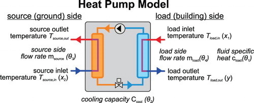
The values of other important parameters for the performance of the water-to-water heat pump can be inferred from the manual of the specific heat pump used in the system and are assumed to be known. The design load flow rate for this specific heat pump type is given as 0.45 m³ h⁻¹, the design source flow rate as 1.2 m³ h⁻¹, and the operational temperature range for cooling is given as 8–20°C for the load side and 5–25°C for the source side, respectively.

All four uncertain parameters are assigned a normal prior distribution, which is a common choice for an informative or weakly informative prior, depending on the chosen variance. Based on the technical specification for the investigated system, we define an expected range and mean value for the four parameters. For the specific heat of the cooling fluid, θ₁, we set the prior mean value to 4.25 kJ kg⁻¹ K⁻¹, which is slightly higher than the anticipated value of water (4.18 kJ kg⁻¹ K⁻¹) so that we expect a shift in the posterior distribution towards the lower value. The prior mean of the rated cooling capacity, θ₂, is set to a slightly lower value (19,100 kJ h⁻¹) than in the heat pump specifications (19,600 kJ h⁻¹), with an expectation of a posterior shift towards higher values. For both parameters, the variance is set to reflect a variability within ±10% of the mean. Regarding the source and load side flow rates, θ₃ and θ₄, we are more uncertain about the true values, so we assume a range of ±20% around the respective mean values of 1800 and 890 kg h⁻¹ for the prior distribution with no precise expectation about the posterior distributions.

Field and computer data used for calibration

The load and source side inlet temperatures of the heat pump represent important boundary conditions for the heat transfer process occurring in the heat pump (Figure 2) and need to be specified as inputs to the TRNSYS model. Accordingly, they are selected as contour state variables x for the calibration process, and different combinations of the two are applied to explore their effect on the calibration results. We will henceforth refer to different combinations of contour states as calibration scenarios.

Measured data for the inlet and outlet temperatures of the heat pump of the Architecture Studio are available as 15 min interval data for a period of two years. From the vast number of measurements available, we select different data sets to examine the influence of outliers and data trends on the calibration results. The selected data only refer to periods when the system operates at full load capacity, and measurements from the first and last two hours of each operation period are disregarded. We select subsets of hourly data instead of using time-series data, which ignores time correlation of the measured data; the effects of time-dependency are expected to be very small in our case, as system components typically have a very low thermal mass.

Each calibration run requires a set of computer simulation results and associated field data. For calibration exercises in this study, we use 10 measurements of the load side outlet temperature y_f at corresponding inlet temperatures x_f (Figure 2). For the computer simulation outputs y_c, the heat pump model is evaluated at the same temperature conditions x_c (= x_f), where field data are available. At each point of x_c, 40 simulation outputs are obtained with varying values for the four unknown model parameters θ using 40 Latin Hypercube samples that cover the above-predefined parameter space.

The field data points and computer outputs used for calibration are displayed in Figure 3 against the two contour state variables. Figure 3 indicates that the supplied temperature to the room – the load outlet temperature – in all data sets lies between 10°C and 18°C, implying that the cool water supply meets the system's design values. The source outlet temperatures (heat rejected to the ground) for data A and B (not shown in Figure 3) are between 30–41°C and 20–32°C, respectively, and thus between 4K and 7K higher than the source inlet. These extremely high values indicate that the system exceeds its design capacity by a large amount.

Figure 3. Measured field data and simulated computer data for the three data sets A, B and C showing the different temperature ranges and trends of each data set across the two dimension of load (upper plots) and source inlet temperature (lower plots).

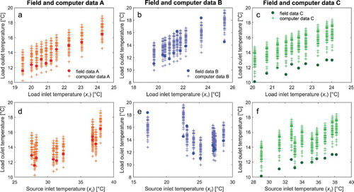
The data sets A, B and C show different trends. Data set A contains field data with an almost linear trend across the operational regime between 19°C and 25°C of load inlet temperature (heat extracted from a room) albeit with some gaps across 25–40°C of source inlet temperature. Data set B has significant noise, as well as gaps in the data across a roughly similar range of load inlet temperature, and a lower range of source inlet temperature (15–30°C), but with some significant outliers (Figure 3(b) and 3(e)). Accordingly, data set B relates to scenarios, where measured field data contain a significant random error. Data set C has fewer outliers from the general trend, but a rather pronounced offset between the field and computer data (Figure 3(c) and 3(f)). From a calibration point of view, data A and B represent cases in which the general trend in the measured data agrees well with the simulation outputs, but a different magnitude of random effects impacts the quality of measurements. Data set C shows a significant difference between field data and computer simulation results (Figure 3(c) and (f)). This relates to scenarios in which the model might not sufficiently represent the true physical behaviour, and we would expect the calibration framework to detect a significant model bias.

Results and discussion

Posterior predictive simulation results

With data sets A, B and C, we first evaluate the ability of the KOH framework to match the model predictions with observations over the range of x. To do so, we also examine the emulator outputs and model bias obtained from the calibration runs. Results from using x₂, the source side inlet temperature, as the only contour state to calibrate the model return posterior distributions identical to the priors (results not shown). Thus, this calibration setup does not enable any interference about the model parameters. This is most likely related to weak correlations between the load side outlet temperature (y, the supplied temperature to the room) and the source inlet temperature (x₂). Accordingly, we focus on two calibration scenarios: (1) scenario ‘1x’: using the load side inlet temperature as the only x and (2) scenario ‘2x’: using both load and source side inlet temperatures as x₁ and x₂ at the same time.

Emulator and model predictions

Figure 4 shows a series of results computed by the model calibrated with data sets A, B and C. In the case of data A, the emulator outputs η(x, θ) of the scenario ‘2x’ follow the observations better, with a slightly tighter range of uncertainty around the mean value (Figure 4(a)). However, the overall model outputs y(x) are similar under both calibration scenarios (Figure 4(b)). This implies that in the absence of information provided by the second contour state variable, the model bias is able to identify the slight discrepancy between the emulator outputs and the observations (Figure 4(c)). The small magnitude of the model bias in both calibration scenarios suggests that the heat pump model appropriately represents all important physical effects for the investigated load and source inlet temperature ranges.

Figure 4. Results for predictive simulations for the emulator (a, d, g), the whole model term (b, e, h) and the model bias function (c, f, i) for data sets A, B and C over the load inlet temperatures (x₁).

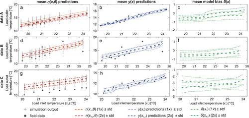
In the case of data set B with more significant outliers and data gaps, neither of the calibration scenarios are able to capture the observations well, and uncertainty around the mean is larger than for data A (Figure 4(d) and 4(e)). This behaviour is typical for GP models, especially when observations are sparse and randomly distributed over x (Williams and Rasmussen 2006). It should be noted that the addition of second contour variable causes an upward trend of predictions. Indeed, Figure 3(e) shows that the load outlet temperature increases between 25°C and 30°C of source inlet temperature. Thus, Figure 4(d) and 4(e) shows that the information provided by the source inlet temperature (x₂) helps to identify the correct trend in the emulator and model predictions in regions, where the first contour variable does not contain enough meaningful information. The magnitude of the model bias function for data B is small for both scenarios, yet it correctly shifts the y(x) predictions towards lower outlet temperatures (Figure 4(e)). This is particularly true for lower inlet temperatures in scenario ‘2x’.

For data C, which contains a significant discrepancy between field and computer data (Figure 3(c) and 3(f)), the emulator and model predictions from the two calibration scenarios are identical (Figure 4(g) and 4(h)). However, the predictions based on scenario ‘2x’ follows the data points more tightly and show a slightly curved prediction function, which is in contradiction with our knowledge about the heat transfer processes in the heat pump component. This effect may be caused by conflicting information from the two contour states.

Model bias predictions

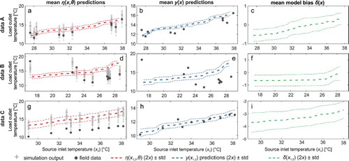
The inadequacy of the model to replicate the measured data C is correctly compensated in both calibration scenarios by the error terms included in Equation (2). However, an opposite trend is observed for the two calibration scenarios: While the model bias from scenario ‘1x’ simply subsumes all differences between emulator predictions and field data (Figure 4(g) and 4(h)), the model bias based on two contour states (scenario ‘2x’) better reflects the expectation of an increasing model bias function (Figure 4(i)). This increasing trend for scenario ‘2x’ is linked to a very similar upward trend in the model bias function over the source inlet temperature (x₂) (Figure 5(i)). Indeed, while the discrepancy between measured and modelled data is constantly increasing over x₁ (Figure 3(c)), the trend over x₂ is less clear and large discrepancies occur for low source inlet temperatures (Figure 3(f)).

Figure 5. Results for predictive simulations for the emulator (a, d, g), the whole model term (b, e, h) and the model bias function (c, f, i) for data sets A, B and C over the source inlet temperatures (x₂).

While all calibration scenarios are statistically valid representations of the model inadequacy of the heat pump model, differences arise from the information contained in different data sets and due to the quality of the data (i.e. gaps and outliers) and the choice of contour states (x₁, or x₁ and x₂). Furthermore, limited data without covering the sufficient range of x impede the ability to make meaningful posterior predictions outside the initial data range, as discussed in detail by Brynjarsdóttir and O'Hagan (2014). Based on similar findings, Li, Augenbroe, and Brown (2016) also suggested that the model bias function should primarily be treated as a way to prevent over-fitting. However, our results show that in case of a significant discrepancy between simulation outputs and field data, such as data C, the derived model bias function can indeed be used to obtain information about the type, magnitude, etc. of this discrepancy. In the next section, we discuss the main hyper-parameters that influence the calculation of the model bias function.

The model bias hyper-parameters

We examine the posteriors of the hyper-parameters relating to the model bias function because they represent important information about the shape and magnitude of model inadequacies that can help improve the physical model. Figure 6 shows the boxplots of the inverse of the prior and posterior distributions for the precision hyper-parameter λ_b (Figure 6(a) and 6(c)), which directly determines the magnitude of the model bias function. The precision λ_bshows no significant changes from the prior for the data sets A and B (Figure 6(a) and 6(c)), while for data set C the model bias increases by a large magnitude (Figure 6(a) and 6(c)), which is the reason for the large negative values in Figures 4 and 5(i).

Figure 6. Prior and posterior probability distributions shown as boxplots for the reciprocal of the precision hyper-parameter λ_b and the correlation hyper-parameters (β_b1 refers to x₁, i.e. load side flow rate, β_b2 refers to x₂, i.e. source side flow rate) of the model bias for the three investigated data sets A, B and C. The centre line represents the median of the posteriors, boxes cover the interquartile range and whiskers include approx. 99% of the obtained posterior samples. The dashed line indicates the magnitude of the prior median value. Please note the parameter values do not represent the absolute value of the error term, as they are inferred from the normalized model data.

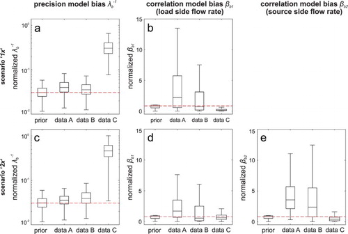
The correlation strength hyper-parameter β_b determines the smoothness of the model bias function in the different dimensions of x (Figure 6(b), 6(d) and 6(e)) with a lower value for β_b indicating a smoother model bias function. As shown, the significantly higher β_b2values for data A and B in Figure 6(e) reflect the more curved form of the model bias and y(x) predictions across the source inlet temperature (x₂) (Figure 5(c) and 5(f)).

Measurement and numerical error

As expected, data set B has higher values for measurement error λ_e (Figure 7(a) and 7(c)). Recall that data set B is the most ‘noisy’ one with many outliers. At the same time, the calibration with two contour states suggests slightly lower random errors (for all data sets), which indicates that with more information available the algorithm is better able to attribute uncertainty to different sources than just the unstructured random error.

Figure 7. Prior and posterior distribution for the reciprocal of the random error λ_e and numerical error λ_en for different data sets on logarithmic scales. The centre line represents the median of the posteriors, boxes cover the interquartile range and whiskers include approx. 99% of the obtained posterior samples. The dashed line indicates the magnitude of the prior median value. Please note the parameter values do not represent the absolute value of the error term, as they are inferred from the normalized model data.

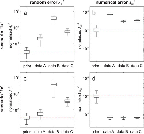
The posterior distributions of λ_en confirm the prior belief about a very small numerical error associated with the discretization of the numerical model and the algorithms used in the computer code. As we are using a set of measurements for the calibration, which does not reflect any specific points in time, the chosen time step of the transient model plays no significant role for the error in the model outcome.

The similarity of the posteriors for the different data set can be explained by the fact that the same code, discretization, algorithms and software are used in all calibration runs. Again, the use of a second contour state variable leads to a significant reduction of this unstructured error.

Inference about uncertain model parameters

This section evaluates the posterior distributions of the four uncertain model parameters. Figure 8 shows the inferred posterior distributions for the four model parameters that exhibit noticeable differences depending on the selected data sets and contour states. As expected, the posterior mode values of θ₁, the fluid specific heat, show a shift towards lower values for all data sets, with a more pronounced shift for data set A than for B and C. Regarding θ₂ and θ₄, the inferred posterior modes for data A also show a larger deviation from the prior into the expected direction of higher values than for data B and C. These observations are consistent for both combinations of x. The posteriors for θ₁ and θ₂ are almost equally improved from the prior for the two scenarios, indicating that more information to further update these posteriors is not provided by the added contour state. θ₃ exhibits posteriors identical to the prior distribution for all data sets under scenario ‘1x’, which indicates either confirmation of the prior knowledge or non-identifiability of this parameter. Indeed, additional calibration runs (results not shown) with different prior distributions for θ₃ always resulted in posteriors identical to the selected priors, which confirms that this parameter is unidentifiable due to a lack of information in the used calibration data.

Figure 8. Prior and posterior distributions as boxplots for the four calibration parameters θ for different data sets. The centre line represents the median of the posteriors, boxes cover the interquartile range and whiskers include approx. 99% of the obtained posterior samples. The dashed line indicates the magnitude of the prior mode value.

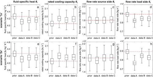
Adding source inlet temperatures as second contour state results in slightly different posteriors for θ₃ and θ₄ under all three data sets. Although the posterior of θ₃ is shifted from the prior for data A with two x, there is no clear knowledge at hand to assess the robustness of the inference about the flow rate on the source side (θ₃) of the heat pump. We also observe a certain variation in the posteriors of θ₄ in the scenario with ‘2x’ particularly for data A, which may indicate that there is a confounding between the source (θ₃) and load (θ₄) flow rate of the heat pump. This un-identifiability of the source flow rate and the confounding between the source and load flow rate may be caused by the structure of the underlying physical model. The heat exchanged across the heat pump is determined by the product of fluid temperature (input data), specific heat capacity and mass flow rates, which are uncertain for both load and source side and have very similar effects on the heat exchange.

A close inspection of the size of the prior and posterior interquartile ranges in Figure 8 reveals that there is only little reduction in posterior uncertainty for the four calibration parameters, while the posterior mode values are successfully updated according to our expectations. This effect was also observed by Freni and Mannina (2010) for posterior distributions of calibration parameters in a water quality model. Also, it must be noted that fixing the remaining unknown parameters at their estimated values may potentially affect the posterior values for the four calibrated parameters, although a study by Heo et al. (2014) showed that the effect of the settings of the other parameters on calibration results is very small.

Influence of model bias on calibration results

Recall that our posterior results for the precision of the model λ_bfor data sets A and B strongly follow the prior (Figure 6(a) and 6(c)). Even with different priors, the posteriors are the same (results not shown). This found non-identifiability of the model precision parameter, λ_b, not only leaves us with no updated knowledge about the potential true magnitude of the model bias function, but also poses a problem for the interpretation of the remaining posteriors. To investigate this further, we run the calibration setup for a set of different priors on λ_b: (GAM(10, 0.03); GAM(10, 0.1), GAM(10, 1), GAM(10, 2.5). These correspond to a magnitude of variation in y caused by the model bias of ∼0.3%, ∼1%, ∼10% and ∼25%, respectively, while preserving the original spread by keeping the shape parameter of the Gamma distribution at 10. Priors of all other (hyper-)parameters remain the same.

The effect of different priors on λ_b on other posteriors is investigated for all three data sets A, B and C under scenario ‘1x’ (Figure 9). The significant changes in the median values of the posteriors of  ₁, θ₂ and θ₄ for data A and B (Figure 9(a–c) and 9(f–h)) indicate that the posteriors distributions of the calibration parameters absorb part of the model bias effect due to the non-identifiable hyper-parameter. Thus, the lack of information about the magnitude of the model precision, λ_b, leads not only to less reliability in the inference of the uncertain model parameters, but also influences the inference of the shape and smoothness of the model bias, represented by β_b in Figure 9(d), 9(i) and 9(o).

Figure 9. Posterior distributions of θ₁, θ₂, θ₄, λ_e⁻¹ and β_b for data sets A, B and C under scenario ‘1x’ for different priors on λ_b (GAM(10, 0.03), GAM(10, 0.1), GAM(10, 0.3), GAM(10, 1), GAM(10, 2.5) corresponding to an amount of variation in y caused by the model bias of ∼0.3%, ∼1%, ∼3%, ∼10% and ∼25%. The base case (∼3%) is indicated in bold. Resulting posteriors for θ₃ are not shown as this parameter is unidentifiable as well, and does not show any changes.

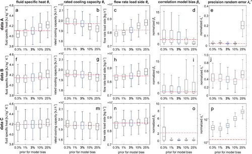
The changes in the corresponding inferred magnitude of the random measurement error, λ_e, for data A and B (Figure 9(e) and (j)) are mostly minor and show no clear trend with increasing prior values for the magnitude of the model bias. For a very high model error of ∼25% of the overall variation in the outcome, y_z, there is a significant change in the posterior of %_e, indicating a larger random error particularly for data set A (Figure 9(e)). As we know that this data set has a rather small measurement error, this observation suggests that there might be a confounding between the identification of the random error and the model bias, as the calibration algorithm partly compensates the suggested large model bias with a large measurement error, in conjunction with a smoother model bias function (Figure 9(d) and 9(e)).

Data C with the large model discrepancy exhibits minor variations in the posteriors for the calibration parameters (Figure 9(l), 9(m) and 9(n)). Even though the large model bias is inferred correctly, the joint posterior distribution from Bayesian inference represents a compromise between the data and the chosen prior distribution, and, consequently, a prior distribution with lower values for λ_b results in a slightly different posterior than a prior with higher λ_b values. The increase in the magnitude of the random error with larger model bias priors again hints at a potential confounding between these two error terms (Figure 9(p)). It appears that part of the suggested large model bias is absorbed by the random error instead, while the model bias only accounts for the strictly linear part of the discrepancy, as indicated by the low β_b values (Figure 9(o)).

These observations highlight the importance of selecting meaningful and representative priors for all hyper-parameters in order to achieve meaningful results from the parameter inference. However, one also has to note that the expectations of a model bias of 0.3 or 25% of the original variation are certainly extreme cases that are less likely to occur in most applications. In contrast to the parameters shown in Figure 9, we observe no significant dependency on λ_b for the hyper-parameters relating the model emulator terms, λ_η and β_η, and for the random numerical error term, λ_en (results not shown), which shows that there is no confounding between these parameters. Overall, the different priors for the model bias precision appear to have a larger impact on the posterior distribution of the random error term than on the calibration parameters in the heat pump model.

Calibration results from randomly sampled data sets

In order to test how the selection of 10 data points from the overall data set affects the calibration results, and how representative the results from the specifically designed data sets (A, B and C) are, we conduct an additional analysis with randomly sampled data sets from the original 4015 measurements available. Overall, 200 sets with 10 random data points each were created and processed according to the same procedure as for data A, B and C using the same prior distributions.

Of the 200 data sets only 152 show convergence after 1000 HMC runs under scenario ‘1x’, while 199 data sets exhibit very good convergence when both source and load side inlet temperature are used as contour states x (scenario ‘2x’). The improvement of convergence with more contour states shows that the additional information contained in the additional x can not only explain different outcomes of y for similar values of one of the x, but also help overcome data gaps in any one dimension of x.

The individual 199 posterior median values, indicated by circles in Figure 10, show that the most likely posterior values of the four calibration parameters cover a rather small range of values, which suggests overall good consistency with the results from the different random data sets (Figure 10(a)–10(d)). For the fluid specific heat (θ₁) and the rated cooling capacity (θ₂), the range of posterior mode values of the random data cover the posterior mode of data A, but slightly differ from the median of data B, which highlights the effect of the quality of this data set. The non-identifiability of the source side flow rate observed for data A, B and C is confirmed by the posterior results from the random data sets (Figure 10(c)). Thus, the non-identifiability is not caused by the way we selected data sets A, B and C and the information contained therein, but rather by a lack of information provided by the whole data set and/or by the structure of the model/emulator. Interestingly, there are a few random calibration runs, where the model bias precision shows a difference between prior and posterior median value (Figure 10(e)), which hints at a slightly improved identifiability compared to data A and B. This suggests that the inferred posterior of the precision of the model bias is very susceptible to the data points used for inference.

Figure 10. Prior distributions and combined histogram plots of all posterior samples from 199 converged calibration runs with 2000 samples each, inferred from the evaluation of the random data sets. The circles indicate the posterior median values of the individual 199 posterior sample sets, while the vertical solid and dashed lines indicate the posterior medians of data A and B, respectively. Note the logarithmic scale on the x-axes for the inverse of the model bias λ_b⁻¹, measurement error λ_e⁻¹ and numerical error λ_en⁻¹.

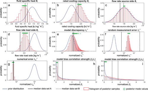
The posteriors of the measurement error, λ_e, from the random datasets exhibit posterior values between the medians of data A and B, which is related to the fact that data A and B were designed to have a particularly low and high measurement error, respectively. For model bias correlation strength parameters, the random data sets yield overall ranges of posterior distributions quite close to the prior, whereas data A and B yield a stronger correlation, in particular with the source side inlet temperature. This difference suggests that the inferred posteriors of the correlation strength parameters may also be susceptible to the data points used for inference.

Conclusions

We apply the Bayesian calibration framework developed by Kennedy and O’Hagan (2001) to the heat pump component of a space cooling system model using point measurements of inlet and outlet temperatures on both load and source sides. By scrutinizing the calibration results from three data sets with different characteristics under different sets of contour state variables and different priors, we assess the capability of the method to provide robust posterior predictions for all unknown parameters.

We found that the framework can reasonably compensate for model discrepancy and measurement error through structured and non-structured error terms under most investigated scenarios. Inference about calibration parameters is quite robust in the presence of large random or structured error terms, which highlights the particular suitability of this method when models do not exactly reflect reality and cases with sparse, noisy data. However, the non-identifiability of the source side flow rate highlights the importance of information contained in the data, and implies that a high sensitivity index is no guarantee for identifiability of a parameter during the calibration process. Thus, we recommend to assess the identifiability and robustness of calibration parameters, which can be easily done by testing different prior information and calibration scenarios.

Analysis of different calibration scenarios shows that adding more information to the Bayesian calibration exercise can have very diverse effects on the resulting model predictions and posterior distributions. Therefore, we emphasize choosing the contour state variables, such as environmental conditions, very carefully. Investigating the posterior information about individual parameters in combination with their priors and other available prior knowledge can be a helpful tool to find the right balance between improving the calibration results and causing unnecessary constraints.

In addition, we uncovered a potential confounding in the inference of the model bias in the heat pump model, which leads to a strong dependency of the joint posterior distribution on the prior information about this parameter. Thus, a more detailed statistical representation of the model bias should be considered for detailed, complex models – especially if the goal of the calibration process is to learn about the model structure and parameter values. In the complete absence of knowledge about these error terms and if the aim of calibration is minimizing the discrepancy between measurements and model outcomes, it might be worthwhile for future studies to compare the performance of the Kennedy & O’Hagan framework to other calibration approaches, such as optimization-based methods. For future studies in the field of Bayesian calibration, more effort should be undertaken to obtain better prior knowledge about the bias of any particular model instead of using standard priors from the literature.

Acknowledgements

Special thanks are given to Prof. Godfried Augenbroe and Qi Li (both School of Architecture, Georgia Institute of Technology, US) for the inspiring and insightful discussions on Bayesian inference and model calibration.

ORCID

Kathrin Menberg http://orcid.org/0000-0002-0517-7484

Additional information

Funding

This study was conducted as part of the ‘Bayesian Building Energy Management (B.bem)’ project funded by the Engineering and Physical Sciences Research Council of the United Kingdom (EPSRC reference: EP/L024454/1).

References

- Arendt, Paul D., Daniel W. Apley, and Wei Chen. 2012. “Quantification of Model Uncertainty: Calibration, Model Discrepancy, and Identifiability.” Journal of Mechanical Design 134 (10): 100908. doi: 10.1115/1.4007390
- ASHRAE. 2002. ASHRAE Guideline 14, Measurement of Energy and Demand Savings. Atlanta.
- Bayarri, Maria J., James O. Berger, Rui Paulo, Jerry Sacks, John A. Cafeo, James Cavendish, Chin-Hsu Lin, and Jian Tu. 2007. “A Framework for Validation of Computer Models.” Technometrics 49: 138–154. doi: 10.1198/004017007000000092
- Berger, James O., Elías Moreno, Luis Raul Pericchi, M. Jesús Bayarri, José M. Bernardo, Juan A. Cano, Julián De la Horra, et al. 1994. “An Overview of Robust Bayesian Analysis.” Test 3 (1): 5–124. doi: 10.1007/BF02562676
- Betancourt, Michael. 2016. “A Conceptual Introduction to Hamiltonian Monte Carlo.” 60.
- Booth, A. T., R. Choudhary, and D. J. Spiegelhalter. 2013. “A Hierarchical Bayesian Framework for Calibrating Micro-Level Models with Macro-Level Data.” Journal of Building Performance Simulation 6 (4): 293–318. doi: 10.1080/19401493.2012.723750
- Brynjarsdóttir, Jenný, and Anthony O'Hagan. 2014. “Learning about Physical Parameters: The Importance of Model Discrepancy.” Inverse Problems 30 (11): 114007. doi: 10.1088/0266-5611/30/11/114007
- Cacabelos, Antón, Pablo Eguía, José Luís Míguez, Enrique Granada, and Maria Elena Arce. 2015. “Calibrated Simulation of a Public Library HVAC System with a Ground-Source Heat Pump and a Radiant Floor Using TRNSYS and GenOpt.” Energy and Buildings 108: 114–126. doi: 10.1016/j.enbuild.2015.09.006
- Chong, Adrian, and Khee Poh Lam. 2017. “A Comparison of MCMC Algorithms for the Bayesian Calibration of Building Energy Models.” In Building Simulation 2017, 1–10. San Francisco: Conference Proceedings.
- Chong, Adrian, Khee Poh Lam, Matteo Pozzi, and Junjing Yang. 2017. “Bayesian Calibration of Building Energy Models with Large Datasets.” Energy and Buildings 154: 343–355. doi: 10.1016/j.enbuild.2017.08.069
- Coakley, Daniel, Paul Raftery, and Marcus Keane. 2014. “A Review of Methods to Match Building Energy Simulation Models to Measured Data.” Renewable and Sustainable Energy Reviews 37 (0): 123–141. doi: 10.1016/j.rser.2014.05.007
- Cobelli, Claudio, and Joseph J. DiStefano. 1980. “Parameter and Structural Identifiability Concepts and Ambiguities: A Critical Review and Analysis.” American Journal of Physiology-Regulatory, Integrative and Comparative Physiology 239 (1): R7–R24. doi: 10.1152/ajpregu.1980.239.1.R7
- Collis, Joe, Anthony J. Connor, Marcin Paczkowski, Pavitra Kannan, Joe Pitt-Francis, Helen M. Byrne, and Matthew E. Hubbard. 2017. “Bayesian Calibration, Validation and Uncertainty Quantification for Predictive Modelling of Tumour Growth: A Tutorial.” Bulletin of Mathematical Biology, 1–36. doi: 10.1007/s11538-017-0258-5.
- Duane, Simon, A. D. Kennedy, Brian J. Pendleton, and Duncan Roweth. 1987. “Hybrid Monte Carlo.” Physics Letters B 195 (2): 216–222. doi: 10.1016/0370-2693(87)91197-X
- Fabrizio, Enrico, and Valentina Monetti. 2015. “Methodologies and Advancements in the Calibration of Building Energy Models.” Energies 8 (4): 2548–2574. doi: 10.3390/en8042548
- Faggianelli, Ghjuvan Antone, Laurent Mora, and Rania Merheb. 2017. “Uncertainty Quantification for Energy Savings Performance Contracting: Application to an Office Building.” Energy and Buildings 152: 61–72. doi: 10.1016/j.enbuild.2017.07.022
- Fisher, Daniel E., Simon J. Rees, S. K. Padhmanabhan, and A. Murugappan. 2006. “Implementation and Validation of Ground-Source Heat Pump System Models in an Integrated Building and System Simulation Environment.” HVAC&R Research 12 (supp1): 693–710. doi: 10.1080/10789669.2006.10391201
- Freni, Gabriele, and Giorgio Mannina. 2010. “Bayesian Approach for Uncertainty Quantification in Water Quality Modelling: The Influence of Prior Distribution.” Journal of Hydrology 392 (1–2): 31–39. doi: 10.1016/j.jhydrol.2010.07.043
- Gelman, Andrew, John B. Carlin, Hal S. Stern, and Donald B. Rubin. 2014. Bayesian Data Analysis. Vol. 2. Boca Raton, FL: Chapman & Hall/CRC.
- Gelman, Andrew, and Donald B Rubin. 1992. “Inference from Iterative Simulation Using Multiple Sequences.” Statistical Science 7: 457–472. doi: 10.1214/ss/1177011136
- Gestwick, Michael J., and James A. Love. 2014. “Trial Application of ASHRAE 1051-RP: Calibration Method for Building Energy Simulation.” Journal of Building Performance Simulation 7 (5): 346–359. doi: 10.1080/19401493.2013.838698
- Guillas, S., J. Rougier, A. Maute, A. D. Richmond, and C. D. Linkletter. 2009. “Bayesian Calibration of the Thermosphere-Ionosphere Electrodynamics General Circulation Model (TIE-GCM).” Geoscientific Model Development 2 (2): 137–144. doi: 10.5194/gmd-2-137-2009
- Heo, Yeonsook, Ruchi Choudhary, and G. A. Augenbroe. 2012. “Calibration of Building Energy Models for Retrofit Analysis Under Uncertainty.” Energy and Buildings 47: 550–560. doi: 10.1016/j.enbuild.2011.12.029
- Heo, Yeonsook, Diane J. Graziano, Leah Guzowski, and Ralph T. Muehleisen. 2014. “Evaluation of Calibration Efficacy Under Different Levels of Uncertainty.” Journal of Building Performance Simulation, 1–10. doi:10.1080/19401493.2014.896947.
- Higdon, Dave, Marc Kennedy, James C. Cavendish, John A. Cafeo, and Robert D. Ryne. 2004. “Combining Field Data and Computer Simulations for Calibration and Prediction.” SIAM Journal on Scientific Computing 26 (2): 448–466. doi: 10.1137/S1064827503426693
- Hoffman, Matthew D., and Andrew Gelman. 2014. “The No-U-Turn Sampler: Adaptively Setting Path Lengths in Hamiltonian Monte Carlo.” Journal of Machine Learning Research 15 (1): 1593–1623.
- Hopfe, Christina J., and Jan L. M. Hensen. 2011. “Uncertainty Analysis in Building Performance Simulation for Design Support.” Energy and Buildings 43 (10): 2798–2805. doi: 10.1016/j.enbuild.2011.06.034
- Kavetski, Dmitri, George Kuczera, and Stewart W. Franks. 2006a. “Bayesian Analysis of Input Uncertainty in Hydrological Modeling: 2. Application.” Water Resources Research 42 (3): W03408. doi:doi: 10.1029/2005WR004376
- Kavetski, Dmitri, George Kuczera, and Stewart W. Franks. 2006b. “Bayesian Analysis of Input Uncertainty in Hydrological Modeling: 1. Theory.” Water Resources Research 42 (3): W03407. doi: 10.1029/2005WR004368.
- Kennedy, Marc C., and Anthony O’Hagan. 2001. “Bayesian Calibration of Computer Models.” Journal of the Royal Statistical Society: Series B (Statistical Methodology) 63 (3): 425–464. doi: 10.1111/1467-9868.00294
- Li, Qi, Godfried Augenbroe, and Jason Brown. 2016. “Assessment of Linear Emulators in Lightweight Bayesian Calibration of Dynamic Building Energy Models for Parameter Estimation and Performance Prediction.” Energy and Buildings 124: 194–202. doi: 10.1016/j.enbuild.2016.04.025
- Li, Qi, Li Gu, Godfried Augenbroe, C. F. Jeff Wu, and Jason Brown. 2015. “Calibration of Dynamic Building Energy Models with Multiple Responses using Bayesian Inference and Linear Regression Models.” Energy Procedia 78: 979–984. doi: 10.1016/j.egypro.2015.11.037
- Li, Qi, Li Gu, G. A. Augenbroe, Jeff Wu, and Jason Brown. 2015. “A Generic Approach to Calibrate Building Energy Models Under Uncertainty Using Bayesian Inference.” 14th conference of International Building Performance Simulation Association, Hyderabad, India.
- Lim, Hyunwoo, and Zhiqiang John Zhai. 2017. “Review on Stochastic Modeling Methods for Building Stock Energy Prediction.” Building Simulation 10 (5): 607–624. doi: 10.1007/s12273-017-0383-y
- Lopes, Hedibert F., and Justin L. Tobias. 2011. “Confronting Prior Convictions: On Issues of Prior Sensitivity and Likelihood Robustness in Bayesian Analysis.” Annual Review of Economics 3 (1): 107–131. doi: 10.1146/annurev-economics-111809-125134
- Manfren, Massimiliano, Niccolò Aste, and Reza Moshksar. 2013. “Calibration and Uncertainty Analysis for Computer Models – A Meta-Model based Approach for Integrated Building Energy Simulation.” Applied Energy 103 (0): 627–641. doi: 10.1016/j.apenergy.2012.10.031
- Menberg, Kathrin, Yeonsook Heo, and Ruchi Choudhary. 2016. “Sensitivity Analysis Methods for Building Energy Models: Comparing Computational Costs and Extractable Information.” Energy and Buildings 133: 433–445. doi: 10.1016/j.enbuild.2016.10.005
- Menberg, K., Y. Heo, and R. Choudhary. 2017. “Efficiency and Reliability of Bayesian Calibration of Energy Supply System Models.” In Building Simulation 2017, 1–10. San Fransisco: Conference Proceedings.
- Mihai, Andreea, and Radu Zmeureanu. 2017. “Bottom-up Evidence-based Calibration of the HVAC Air-side Loop of a Building Energy Model.” Journal of Building Performance Simulation 10: 105–123. doi: 10.1080/19401493.2016.1152302
- Morris, Max D. 1991. “Factorial Sampling Plans for Preliminary Computational Experiments.” Technometrics 33 (2): 161–174. doi: 10.1080/00401706.1991.10484804
- Muehleisen, R. T., and Joshua Bergerson. 2016. “Bayesian Calibration – What, Why and How.” International High Performance Buildings Conference. Purdue University.
- Mustafaraj, Giorgio, Dashamir Marini, Andrea Costa, and Marcus Keane. 2014. “Model Calibration for Building Energy Efficiency Simulation.” Applied Energy 130 (0): 72–85. doi: 10.1016/j.apenergy.2014.05.019
- Neal, Radford M. 2011. “MCMC Using Hamiltonian Dynamics.” Handbook of Markov Chain Monte Carlo 2: 113–162.
- Neto, Alberto Hernandez, and Flávio Augusto Sanzovo Fiorelli. 2008. “Comparison between Detailed Model Simulation and Artificial Neural Network for Forecasting Building Energy Consumption.” Energy and Buildings 40 (12): 2169–2176. doi: 10.1016/j.enbuild.2008.06.013
- Niemelä, Tuomo, Mika Vuolle, Risto Kosonen, Juha Jokisalo, Waltteri Salmi, and Markus Nisula. 2016. “Dynamic Simulation Methods of Heat Pump Systems as a Part of Dynamic Energy Simulation of Buildings.” Paper presented at the Proceedings of BSO2016: 3th Conference of International Building Performance Simulation Association England, Newcastle, England.
- Omlin, Martin, and Peter Reichert. 1999. “A Comparison of Techniques for the Estimation of Model Prediction Uncertainty.” Ecological Modelling 115 (1): 45–59. doi: 10.1016/S0304-3800(98)00174-4
- Reddy, T Agami, Itzhak Maor, S. Jian, and C. Panjapornporn. 2006. “Procedures for Reconciling Computer-Calculated Results with Measured Energy Data.” ASHRAE Research Project 1051-RP: 1–60.
- Roy, Christopher J., and William L. Oberkampf. 2011. “A Comprehensive Framework for Verification, Validation, and Uncertainty Quantification in Scientific Computing.” Computer Methods in Applied Mechanics and Engineering 200 (25–28): 2131–2144. doi:10.1016/j.cma.2011.03.016.
- Silva, Arthur Santos, and Enedir Ghisi. 2014. “Uncertainty Analysis of the Computer Model in Building Performance Simulation.” Energy and Buildings 76: 258–269. doi: 10.1016/j.enbuild.2014.02.070.
- Sun, Kaiyu, Tianzhen Hong, Sarah C. Taylor-Lange, and Mary Ann Piette. 2016. “A Pattern-Based Automated Approach to Building Energy Model Calibration.” Applied Energy 165: 214–224. doi: 10.1016/j.apenergy.2015.12.026.
- Tian, Wei. 2013. “A Review of Sensitivity Analysis Methods in Building Energy Analysis.” Renewable and Sustainable Energy Reviews 20 (0): 411–419. doi:10.1016/j.rser.2012.12.014.
- Tian, Wei, Song Yang, Zhanyong Li, Shen Wei, Wei Pan, and Yunliang Liu. 2016. “Identifying Informative Energy Data in Bayesian Calibration of Building Energy Models.” Energy and Buildings 119: 363–376. doi: 10.1016/j.enbuild.2016.03.042.
- Wang, Shuchun, Wei Chen, and Kwok-Leung Tsui. 2009. “Bayesian Validation of Computer Models.” Technometrics 51: 439–451. doi: 10.1198/TECH.2009.07011
- Williams, Christopher KI, and Carl Edward Rasmussen. 2006. “Gaussian Processes for Machine Learning.” The MIT Press 2 (3): 4.
- Yang, Zheng, and Burcin Becerik-Gerber. 2015. “A Model Calibration Framework for Simultaneous Multi-level Building Energy Simulation.” Applied Energy 149: 415–431. doi: 10.1016/j.apenergy.2015.03.048