Development of building thermal environment emulator to evaluate the performance of the HVAC system operation

Abstract

A “performance gap” arises when the actual value of building energy consumption during the operational phase deviates from the value predicted using simulation during the design phase. One cause of this performance gap is that operation is not ideal, as assumed in the simulation, and the control of the heating, ventilating, and air conditioning (HVAC) system is not optimized. These problems occur because the operator has not been trained sufficiently and/or the building automation system is not working as intended by the developer. Both problems are fundamentally caused by the fact that the quality of building operation cannot be quantitatively evaluated by comparison with other buildings because a building is a heterogenous, single-item product. To address the performance gap problem, we developed a method for quantitatively evaluating building operation using a precise simulation based on a thermal environment emulator. The emulator software was developed using the BACnet protocol as an interface to the real world and includes an occupant behavior model to enable the assessment of operation in terms of thermal comfort as well as energy performance. In this paper, we report on the program and network structure of the proposed emulator. In addition, we show the concrete results of changing the operational control, and we assess changes in energy performance and comfort from the perspective of Pareto efficiency.

Keywords:

• emulator
• HVAC
• optimization
• BACnet
• occupant behavior
• operation

1. Introduction

The household and services sectors, both of which relate to buildings, contribute about 40% of the world’s total final energy consumption (International Energy Agency 2008). Thus, from environmental and energy efficiency standpoints, promoting energy conservation in buildings is of great significance. In recent years, a new paradigm, the zero-energy building (ZEB), has been proposed and advanced in a number of countries (European Parliament 2010; DOE 2015; METI 2015).

Several simulation software packages have been developed to improve the energy performance of buildings through improved design and operation (Trčka and Hensen 2010). Verhelst et al. (2017) argue that such software should be applied throughout a building’s life cycle, particularly to address the “performance gap” that arises when the actual consumption during operation deviates from the energy consumption simulated during the design phase (Wilde 2014). Khoury, Alameddine, and Hollmuller (2017) cited two causes for such divergence: suboptimal operational stage control and suboptimal usage conditions. Mills et al. (2004) collected the commissioning results for 150 existing buildings and reported that analyzing the building operation could reduce energy consumption by an average of 18%.

Energy consumption during the operational phase is significantly affected by building use and the manner in which the heating, ventilating, and air conditioning (HVAC) system is operated. Therefore, even in buildings of similar applications and sizes, actual energy consumption varies widely (see survey data by Takaguchi et al. 2012). Thus, stabilizing the operation of the HVAC system controller can potentially result in lower, more stable energy use. For this purpose, the operational performance must be quantitatively evaluated. However, because buildings are very heterogeneous, fairly comparing their operational performance is difficult. Even when the energy consumption of a specific building is low, it will be unclear as to whether and to what degree this low consumption is the result of good operation, new equipment, or effective behavior on the part of the building users.

In this paper, we propose an emulator system that quantitatively evaluates building operation using a simulation model. We created a whole-building simulation model that can respond in real time to the actions of the operator or building automation system. As it is a simulated (i.e. virtual) building, any number of buildings can be created with exactly the same HVAC system, occupant behavior, outside air conditions; thus, the quality of operation in these buildings can be fairly compared. The “standard operation building model” and “operation improved building model” are executed in parallel in the same emulator system. By comparing the simulation results of both models, the operation can be evaluated from both aspects of energy performance and thermal comfort. When such an evaluation method is established, it is useful to the owner for selecting a building operation manager or a building automation system. Further, by improving technology as a result of competition, the performance gap problem will be reduced. We believe that a championship can be held using such an emulator system that fairly compares operational performance, and we have actually begun planning the World Championship in Cybernetic Building Optimization (WCCBO). In the WCCBO, several cyber buildings (emulator systems) will be uploaded to a server so that each participant can try to optimize buildings under the same conditions.

In this paper, we report on the architecture of the emulator system, the composition of its network, and the method it uses to evaluate energy use and occupant comfort.

2. Review of research related to emulator construction

An emulator is a simulation model that verifies the operation of equipment by creating a virtual structure (here, a building) that can operate in real time through bidirectional connection to its real-world counterpart. According to our working definition, an emulator can simulate and replace an element when multiple elements are combined to form a large system. For building optimization, we must consider a system consisting of the occupants, HVAC system, building structure, building managers, building automation system, etc. The emulator developed in this research simulate a building structure, an HVAC system, and an occupant. Because the emulator must be able to replace the object to be emulated, the most important function is its ability to communicate properly with the other elements. Therefore, in this case, the possibility of communication with the building manager or building automation system is important, and not the communication with the real building, which was replaced by the emulator. We use the term “emulator” based on these criteria.

The first digital emulators were designed in the 1960s for use in the aviation field as flight simulators for training pilots (Page 2000), and academic research on building equipment emulators began around the 1990s. An example of early efforts to simulate building equipment is Annex 17 of the IEA ECBCS (Lebrun and Wang 1993; IEA 1997), in which an emulator is proposed for the general purpose of verifying the operation of building energy management systems (BEMS). A six-country team (including the United States, the United Kingdom, France, the Netherlands, Finland, and Belgium) prototyped emulator using two dynamic simulators, TRNSYS and HVACSIM+, which were described in detail by Vaezi-Nejad et al. (1991).

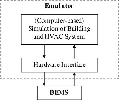
The basic configuration of the emulator for evaluating BEMS in Annex 17 is shown in Figure 1. The Annex lists several required specifications for the emulator, including 1) the capability to run a simulation in real time; 2) the ability to realistically model the dynamic behavior of the controls and actuators; and 3) an interface linking the real BEMS to the simulation model. The emulator is identified as being applicable to: 1) examining the control software and hardware; 2) assessing the control strategies and control algorithms; 3) fine-tuning the pre-set values; and 4) training operating personnel. The approach and methodology of the present study are closely related to the fourth purpose. As discussed in detail by Lazarova-Molnar et al. (2016), most past research on emulators involved fault detection diagnosis (FDD), which is treated in Annex 25 following Annex 17 (IEA 1999). However, very few studies have focused on the training or educational uses of emulators (Neuman 2011, 2012; Serra et al. 2017).

Figure 1. Building emulator used to evaluate a control system.

Kelly and May (1990) reported in detail an emulator-based method for testing BEMS, outlining the major BEMS functions and hardware and software configurations available at that time and describing the evaluation criteria, conditions, and results of BEMS testing. They noted that BEMS algorithms should be judged against three main criteria: (1) energy savings, (2) occupant comfort, and (3) BEMS error. Much of the literature on optimization in recent years has also argued for evaluation in terms of both energy use and comfort (Shaikh et al. 2014; Granderson et al. 2018; Prada, Gasparella, and Baggio 2018). Shaikh et al. (2014) reviewed 121 studies on building optimization and reported that 105 of these studies involved a dual evaluation of the energy performance and thermal comfort.

In the 1990s, the limits of computer performance hindered the development of emulators. For example, a report by Haves et al. (1991) on the emulator-based testing of an air-handler reset strategy and a reheat coil control valve cited three problems with the emulator available at that time, namely, a lack of pressure drops in the air distribution system model, the low level of detail in their dynamic coil models, and slow serial communication. Kärki and Lappalainen (1994) also pointed out problems with communication speed and proposed a new data-processing system in which TRNSYS inputs/outputs were connected to hardware to reduce the time delay. In the early days of research, only certain parts of the HVAC system were often modeled to overcome the limitations of computer performance. In Annex 17, only one zone and its accompanying sensors and equipment were subjected to modeling, and Zheng et al. (1999), Larech et al. (2002), and Watanabe et al. (2007) targeted similar ranges for modeling. However, computer performance has improved significantly since the turn of the century, and an entire building can now be emulated real time.

In addition to improved computer performance, significant progress since the 1990s in open communication protocols such as BACnet (ASHRAE 2016) has contributed considerably to the informationalization of buildings. Whereas the emulators developed in Annex 17 use a specific hardware interface to connect the virtual and real worlds, significant improvements in emulator versatility can be attained through the development of open protocols that can be implemented through software interfaces via BACnet. Bushby et al. (2001; 2010) developed an integrated emulator, the “Virtual Cybernetic Building Testbed” (VCBT), to simulate air conditioning and fire systems. The VCBT employs a hybrid system in which a conventional hardware interface and a software interface by BACnet are implemented.

The spread of model-based development in this industry is also deeply related to the development of emulators. This is a method for advancing the development of the control system by connecting with the physical simulation model as well as the real-world machine, and it enables simultaneously developing the hardware and control system in the product. In other words, the physical simulation model acts as an emulator. In Annex 60 (IEA 2017), an HVAC system emulator was developed using Modelica, an open-source software application that is the de facto standard in model-based development. In recent years, automatic conversion from building information modeling (BIM) data to Modelica has also been actively researched (Kim et al. 2015; Wimmer et al. 2015; Pinheiro et al. 2018).

Based on the research findings discussed above, the functions necessary for the emulator developed in this study are given as follows.

As the interface to the external world, a software interface via BACnet was adopted in place of a hardware interface. Traditionally, emulators in the field of building equipment have used hardware interfaces, which differs from this emulator, which completes everything using software. By implementing the entire emulator system on software, a system could be developed that can be copied and distributed simply and inexpensively and that enables simultaneously testing multiple operations. This also makes it easier to remotely test the system over the Internet. The program and network structure used in the software implementation are discussed in section 3.

The system evaluates performance in terms of not only energy performance but also thermal comfort. In many cases, there is a trade-off between energy savings and comfort, so they must be concurrently evaluated. To evaluate thermal comfort, the thermal environment of each occupant must be understood, and the entire zone of the building must be modeled as a simulation target. Meanwhile, to evaluate energy consumption, the entire HVAC system must be modeled, including the heat source. Thus, the modeling target comprises the building’s thermal load, the temperature and humidity in its respective zones, the HVAC system, including the air conditioners, and the heat sources, i.e. the complete thermal environment system of the building. In section 4, in addition to the method for evaluating energy and comfort, we report the results of the evaluation by changing several control methods.

3. Implementation of the BACnet communication function

3.1. Program structure of real-time communication

A conventional simulation of a heat load and HVAC system will typically first determine the schedule of operation and then compute their respective solutions, with no results returned until all of the calculations have been completed. However, because an emulator must respond in real time, it cannot employ this type of batch processing. Instead, the emulator must switch controls and obtain the current state of the model with the desired timing. To this end, a function can be implemented to perform BACnet communication via asynchronous processing. The emulator uses an object-oriented language to divide functions into two clear classes—one for calculating the physical HVAC equipment state and one for controlling the equipment.

A Unified Modeling Language (UML) class diagram of a cooling tower system is shown in Figure 2 as an example. In a conventional energy simulation program, control and physical calculations are generally included in the same class or sub-routine; in the proposed emulator, these functions are divided into a “CoolingTower” class that performs physical calculations and a “CoolingTowerController” class that performs control calculations. In the CoolingTower class, the cooling water outlet temperature and fan electric power are calculated based on the on/off state of the fan, the inlet temperature and flow rate of the cooling water, and the wet-bulb temperature of the outdoor air. Instead of using CoolingTower to change the on/off state of the fan or the flow rate of the cooling water depending on the temperature of the cooling water, CoolingTowerController is used to set the on/off status of the fan based on the set point temperature. However, the ideal temperature of the cooling water cannot be observed directly. Instead, the thermometer model results, which are time-delayed and of limited precision, must be used; this also applies to the electricity consumption of the fan. Because CoolingTowerController must be capable of performing communication with any timing, functions enabling operation are implemented as BACnet devices. Because such functions are commonly required for controllers other than the cooling tower, an “IBACnetDevice” interface is defined and implemented. IBACnetDevice has two functions: 1) managing the control value inside the emulator and 2) BACnet communication outside of the emulator at an arbitrary timing. IBACnetDevice receives measured variables (temperature, electricity, etc.) from the device to be controlled and sets manipulated variables (on/off state, motor rotation rate, etc.) at constant time intervals. This receiving and setting processing must be executable asynchronously through BACnet communication with the client; in the proposed emulator, asynchronous processing is achieved using the C# multi-thread function.

Figure 2. UML class diagram of a cooling tower system.

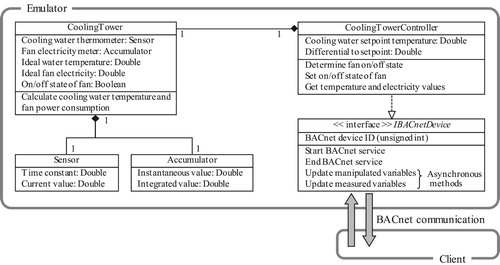
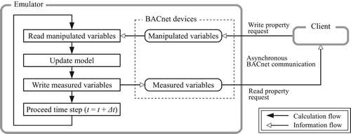
Figure 3 shows the computational flow and timing of information transmission, in which the BACnet devices of the emulator store manipulated and measured variables. The model is updated based on the manipulated variables, while the state (temperature, humidity, electricity, water consumption, etc.) of the model is measured using sensors. After the measured values have been written to the measured variables of the BACnet devices, the next time step is calculated. Because BACnet devices can perform asynchronous BACnet communication, clients connecting to the emulator can rewrite manipulated variables and read the values of measured variables with arbitrary timing.

Figure 3. Calculation flow and timing of information transmission.

As will be described later, the calculation time step of the simulation is 10 s. Therefore, when the BACnet communication is performed at shorter time intervals, the measured values from the emulator do not change. Because the communication interval between the current central Human Interface Module (HIM) and the local device is about one minute, there is no problem at this time interval in consideration of the HIM. However, the local Intelligent Controller (ICont) is likely to communicate and control in less than 10 s. Therefore, when testing such control, shorter calculation time intervals must be set.

3.2. Network configuration of remote communication

To remotely evaluate the operation, it is useful for the emulator system to be able to communicate using the BACnet/IP, which requires specification of the network addresses of the BACnet devices. Each network address is given as a four-octet IP address followed by a two-octet UDP port number. Normally, 47808 (“xBAC0” in hexadecimal) is used as the port number, which is identified by the IP address. However, when multiple BACnet devices are virtually coexistent within a single software package such as an emulator, assigning different IP addresses is difficult, in which case it is permissible to identify the BACnet device by making the port number unique (ASHRAE 2016). The IP addresses of the approximately 100 BACnet devices included in the proposed emulator are equivalent to those of the computer on which the emulator runs and are identified by the port number.

Because an IP router will generally block broadcast messages and the use of unauthorized ports, communication via the Internet requires modifying the normal BACnet. There are two major methods for implementing such a modification: using a BACnet/IP broadcast management device (BBMD) or using an Internet virtual private network (VPN).

A BBMD sends all received broadcast messages through the IP router to a partner BBMD. To use such devices in the emulator, however, a BBMD (either hardware or software) must be provided for each IP subnet, and the IP addresses of all of the BBMDs must be configured correctly. To enable this broadcast, the settings on the server (emulator) side must be updated each time the client changes. In addition, a port must be opened for communication with the BBMD.

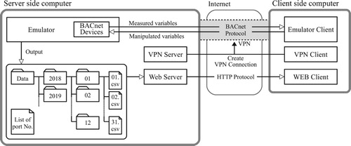
A VPN is a private network that is virtually established on a public network. Using a VPN, a server and client can communicate as if they were on the same local network. Although a port for a VPN must be opened, because this is a communication technology commonly used in a wide variety of fields, there will likely to be fewer barriers to doing so than for opening ports for BBMD communication. Based on this advantage, the proposed emulator system implements remote communication via VPN using the network configuration shown in Figure 4, in which a connection is established by installing VPN software to the server and client and is used to perform BACnet communication. The past operational data of the emulator and a list of BACnet device port numbers are downloadable from a Web server.

Figure 4. Network configuration of the emulator system.

4. Building operation evaluation criteria

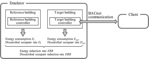
As described in section 2, many building optimization studies have evaluated both energy consumption performance and indoor comfort. The emulator developed in this study calculates two building models in parallel so that their respective performance results can be output in real time. This parallel computational structure is shown in Figure 5. The two models in the emulator are “Reference building” and “Target building.” As shown in Figure 2, each model is divided into a physical calculation and a control calculation component. Only the Target building controller can perform BACnet communication with the client, with the Reference building control retaining the default control values, which do not change. As will be described later, the model expresses elements that change stochastically such as occupant behavior and weather conditions. Because the emulator uses a pseudorandom number generator with a constant random seed, two models will produce exactly the same results if the control is not changed. Thus, any differences in energy consumption E [GJ/a] or occupant dissatisfaction rate D [-] between the two models must be induced by a change in control. By comparing the calculated results for E and D produced by the respective models, the energy reduction rate (ERR [-]) and dissatisfied occupant reduction rate (DRR [-]) can be calculated using Eq. 1 and 2, respectively: (1) $ERR=\frac{E_r-E_{opt}}{E_r},$(1) (2) $DRR=\frac{D_r-D_{opt}}{D_r}.$(2)

Figure 5. Computational flow of energy consumption and indoor comfort performance calculations.

When the emulator system is applied to optimize a specific real-world building, the calculation results of the simulation model (reference building) must match the real monitored data of the real building. The process of tuning the model’s parameters to reduce the mismatch is known as model calibration, and many studies have tackled this problem (O’Neill and Eisenhower 2013; Chaudhary et al. 2016; Qiu et al. 2018). Although model calibration is an important process for increasing the effectiveness of the simulation, this research mainly focused on developing a method for evaluating operation. As this emulator system is not always used in combination with real buildings, we do not deeply investigate the problem of model calibration of the reference building in this paper.

4.1. Evaluation of energy reduction

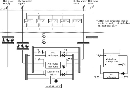
To test the emulator, a seven-story Tokyo tenant office building of a standard building type defined under Japan’s energy conservation law (the Act on Rationalizing Energy Use) was simulated. Figure 6 and Figure 7 show a reference floor plan and the heat source and air conditioning systems used in the building, respectively. The heat source machinery comprises air heat-source heat pump (AHP) with water heat storage tanks and direct-fired absorption chillers. Two air-handling units (AHUs), a perimeter and an interior unit, are installed in both the north and south rooms.

Figure 6. Reference floor plan.

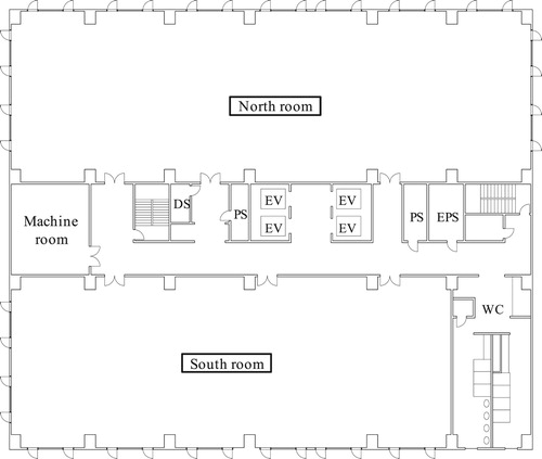
Figure 7. Heat source and air conditioning systems.

The emulator uses Eq. 3 to evaluate the building’s primary energy consumption E_prim [MJ] in terms of electricity C_e [kWh], gas consumption C_g [m³], and water use C_g [m³]: (3) $E_{prim}=R_e{C}_e+R_g{C}_g+R_w{C}_w,$(3) where R_e [MJ/kWh], R_g [MJ/m³], and R_w [MJ/m³] are the primary energy factors. Although these coefficients differ depending on the country or region, R_e = 9.76 MJ/kWh, R_g = 45 MJ/m³, R_w = 8.5 MJ/m³ are often used in Japan. The computational methods to model the energy consumption of equipment are generally similar to those used by conventional models. The HVAC model uses a thermal load calculation library (Togashi 2016) that has been verified by BESTEST (Judkoff and Neymark 1995; Togashi and Tanabe 2009) with static equipment models verified according to SHASE guidelines (SHASE 2016; Ono, Ito, and Yoshida 2017). Table 1 summarizes the calculation method and features of the component models included in this simulator. Many of these are well-known models described in the references in Table 1, but we have mainly added two calculations for use in the emulators: one is the model of the piping and ducting network, and the other is the model of the dynamic behavior of the equipment.

Table 1. Summary of the calculation method and features of the component models included in this simulator.

Component		Outline of the calculation method	Reference
HVAC system	Absorption chiller	Identify the operating point on the Dühring chart by calculating the thermal properties of the lithium bromide solution. The theoretical double-effect absorption refrigeration cycle is expressed to estimate the influence of changes in the temperature and flow rate of cooling and chilled water on efficiency. First-order lag is added to the static model (described later).	Togashi (2016)
	AHP	The model is based on the performance curve. The structure of the performance curve equation is derived from the equation of the theoretical coefficients of the heat pump cycle (COP = Tc / (Th-Tc)). The equation includes the outlet temperature of the hot and chilled water so that the influence of simultaneous fluctuations in the temperature and flow rate of water can be expressed. First-order lag is added to the static model (described later).	Togashi (2018b)
	Cooling tower	The model expresses sensible and latent heat transfer based on enthalpy potential as the driving force. The Number of Transfer Units (NTU) method is used to determine the effectiveness of the heat exchanger. First-order lag is added to the static model (described later).	Donald and Howard (1961)
	Pump and Fan	The characteristic of the pressure rise is approximated by a polynomial of the volumetric flow rate. The power consumption is calculated from the flow rate, pressure rise, and total efficiency (the product of inverter, motor, and pump efficiencies). The calculation method for piping and duct network flow will be described later in detail.	Togashi (2016)
	Cooling and heating coils	The heat transfer is calculated by switching the heat transfer coefficients for the regions of the dry coil and wet coil. The heat transfer coefficients are estimated based on the water and air flow speeds, which are provided by the manufacturer.	JABMEE (1992)
	Rotary heat regenerator	The NTU method is used to determine the effectiveness. The NTU value is estimated with Coppage’s formula.	Coppage(1953)Bahnke and Howard (1964)
	Plate fin heat exchanger	The NTU method is used. The effectiveness is calculated using the analytical solution of a counterflow-type heat exchanger.	Kays and London (1998)
	Water heat storage tank	The model is the temperature-stratified thermal storage tank model, which can simulate variable input conditions (changes in the flow rate temperature of the inlet water). The model is a dynamic model whose temperature distribution in the tank is expressed by the advection–diffusion equation. The parameters are estimated from the dimensionless number obtained experimentally.	Tsujimoto, Sagara, and Nakahara (1981)Kitano, Iwata, and Sagara (2005)
Component		Outline of the calculation method	Reference
	Damper and water valve	The resistance coefficient is calculated from three conditions: the relative position, weighting factor for the linear term of the flow resistance coefficient, and leakage parameter. An electronic actuator is installed, and the position is assumed to move proportionally to the time step.	Clark (1985)Haves (1994)
	Sensors	Sensors are modeled by a first-order differential equation with a single time constant. Based on the manufacturer’s technical data, the time constants were set as follows: water temperature, 50 s; room air (0.15 m/s) temperature, 270 s; room relative humidity, 45 s; duct air (2.0 m/s) temperature, 60 s; and CO2 concentration, 180 s. The time constant of the pressure sensor was regarded as 0 s.	Clark (1985)
	PI controller	The model is based on the velocity algorithm, which prevents integral windup.	SHASE (2001)
Thermal load	Wall heat transfer	Set mass points in each layer of the wall and solve one-dimensional unsteady heat conduction using the difference method. The heat flow on the wall surface is divided into radiation and convection.	–
	Window	Solar radiation is divided into direct radiation and diffuse radiation. Glazing properties (reflectance, absorptance, and transmittance) are calculated from the incidence angle function. Short-wave energy is allocated according to the wall and floor position and surface area ratio.	–
	Shading	The optical properties of parallel slats blind are calculated based on slat geometry and angle.	ISO (2003)
	Zone temperature	The zone temperature is simultaneously solved with the temperature of the walls using the difference method, reflecting heat flow by ventilation, heat flow by inter-zone ventilation, internal heat generation, and heat capacity of the zone. By using coefficients analytically obtained using an inverse matrix of the inside wall heat transfer, long-wave radiation between wall surfaces is also simultaneously solved.	Udagawa (1993; 1997)
	Occupant behavior	Described later in detail.	–
	Thermal comfort	Described later in detail.	–
Numerical calculation		Root finding of nonlinear function:Golden section (one-dimensional), Newton Raphson (multi-dimensional)Linear algebraic equations: lower–upper (LU) decompositionRandom number generation: Mersenne twister	Matsumoto and Nishimura (1998)

4.1.1. Modeling the piping and duct network flow

As Haves et al. (1991) pointed out, many simulations currently do not model the airflow network in detail to express the mutual influence of variable air volume (VAV) units. Instead, conventional energy simulation programs simply pass the sum of the required airflow rates of each VAV unit to the fan model. In such a model, it is not possible to track proportional–integral–derivative (PID)-controlled factors such as the opening degree of the VAV unit, the rotational speed control of the fan, the control of the two-way valve in the piping network, or the control of the rotational speed of the pump. To track these controls, the pressure of all of the nodes of the network must be accurately calculated. Zhu et al. (1994) and Niwa, Watanabe, and Nakahara (1995) tested a method for building optimization fault detection diagnosis (BOFD) in which a detailed airflow model is added to HVACSIM + . In this model, the relationship between the pressures in the respective nodes and the flow rates in the channels is expressed as a nonlinear equation. Because nonlinear simultaneous equations will not obtain solutions in all situations, the proposed emulator uses equivalent resistances to reduce the network variable prior to numerical calculation.

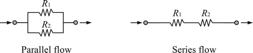
Assuming that the pressure loss in the flow path is proportional to the square of the volumetric flow rate, as shown in Eq. 4, the equivalent resistance of the parallel and series flows shown in Figure 8 can be calculated via Eq. 5 and Eq. 6, respectively. As this is an analytical solution, the accuracy of the flow rate and pressure calculation results does not decrease. By using this relationship, a complicated circuit network can be simplified. (4) $\mathrm{\Delta }P=R{Q}^2,$(4) (5) $R_{1+2}=R_1+R_2$(5) (6) $R_{1+2}=1/{\left(\sqrt{1/R_1}+\sqrt{1/R_2}\right)}^2$(6)

Figure 8. Parallel flow and series flow.

Figures 9 and 10 provide an illustrative example showing a duct diagram of the north room and the structure of the air conditioner unit, respectively. A circuit network expression of the air conditioner and ducting of the perimeter zone is shown in Figure 11. To avoid solving nonlinear simultaneous equations with respect to pressure at 14 nodes, the problem can be simplified using equivalent resistances. For instance, the equivalent resistance (R_18→19), as calculated in Eq. 7, can be used to represent the series resistance of the flow path of VAV-6. The equivalent resistance R_18→19 and the flow path of VAV-5 are arranged in parallel and can be reduced to the equivalent resistance R_16→19, as given by Eq. 8. In a similar manner, all of the equivalent resistances from VAV-1 to VAV-6 can be obtained. Figure 12 shows a simplification of Figure 11 using this equivalent resistance method, through which the number of unknown variables has been reduced from 14 to five, with a corresponding increase in the stability of numerical calculation. The same numerical calculation approach to reducing the number of variables using equivalent resistances is also applied to the piping network. (7) $R_{18\to 19}=R_{18}+R_{vav6}+R_{19},$(7) (8) $R_{16\to 19}=R_{16}+\frac{1}{{\left(\sqrt{1/R_{18\to 19}}+\sqrt{1/\left(R_{vav5}+R_{17}\right)}\right)}^2}.$(8)

Figure 9. North room duct diagram.

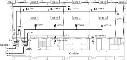
Figure 10. AHU structure.

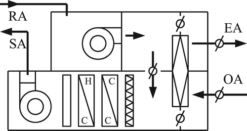
Figure 11. Circuit network of duct and AHU of north perimeter zone.

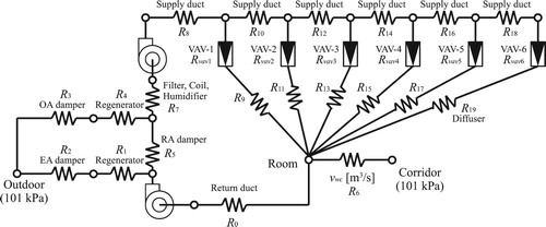
Figure 12. Simplified equivalent resistance circuit network of duct and AHU of north zone.

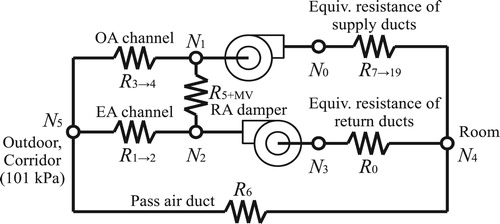
One method for solving the circuit is to make the pressure an unknown variable; another is to make the flow rate an unknown variable. In this model, the method for making the pressure unknown was used. Here, if the resistance coefficient R of Eq. 4 becomes zero, the flow rate Q diverges to infinity, so the numerical calculation fails. Therefore, we assumed that R is a number greater than zero. Even if the opening rate of the damper or the valve, which is treated a variable resistor, is 100%, as the resistance does not become zero, such assumption (0 < R) is consistent with the real HVAC system.

4.1.2. Calculating the dynamic behavior of the equipment

To investigate the timing of machine actuation and termination or the parameters of PID control, the heat capacity and time delay of the building equipment must be expressed. The proposed emulator expresses the first-order lag by adding a heat capacity parameter to the static model of each equipment component, as in Eq. 9. Solving this differential equation produces Eq. 10. 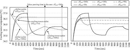(9) $C\frac{dT\left(t\right)}{dt}=m{c}_p\left(T_i-T\left(t\right)\right)+K\left(T_{amb}-T\left(t\right)\right),$(9) (10) $\begin{array}{rl}T\left(t\right)& =A+\left(T\left(0\right)-A\right)\exp \left(-Bt\right),\\ A& =\frac{m{c}_p{T}_i+K{T}_{amb}}{m{c}_p+K},\\ B& =\frac{m{c}_p+K}{C}.\end{array}$(10) where C [kJ/K] is the heat capacity of the equipment, m [kg/s] is the mass flow rate of water, c_p [kJ/(kg·K)] is the isobaric specific heat of water, T_i [K] is the inlet water temperature, T(t) [K] is the temperature of water in the equipment, T_amb [K] is the ambient temperature, and K [kW/K] is the heat loss coefficient. Although Eq. 9 can be adopted for use with multiple equipment components, and the resulting simultaneous ordinary differential equations can be solved, the calculation complexity is reduced by solving Eq. 9 as Eq. 10. The values of the variables obtained by solving Eq. 10 are common for all equipment components over the short time interval ΔT_pass [s]. However, this is a closed-form solution that assumes m and T_i to be constant; when the time interval for passing the value of variables is too large, the error increases. Therefore, the relationship between the passing time interval and the error magnitude was tested for the operation expected to have a very large error. This is the case when the chiller and the cooling tower are turned off, and only the cooling water pump remains in operation. Further, this is when the cooling water of 32 and 37 °C start to mix directly. Table 2 shows the values of the parameters for checking the magnitude of the error. These values are set based on the technical data from the manufacturer and the experience that it takes about 30 min to start up the absorption chiller system.

Table 2. Values of the parameters for checking the magnitude of the error.

Parameters	C	K	mcp	Tamb
Chiller	114,270 kJ/K	0.89 kW/K	160.5 kW/K	35 °C
Cooling tower	8,929 kJ/K	0.14 kW/K	(const.)	(const.)

Figure 13 shows the relation between the value passing time interval and cooling water temperature calculation results. The left side shows the transition of the outlet water temperatures of the chiller and cooling tower when ΔT_pass = 360 s and ΔT_pass = 1 s. This figure shows that when the time interval is large (360 s), as the temperature of the connected equipment is regarded as a constant, the calculation result becomes unstable when the temperature change is so large. The figure on the right is the change in the calculation result for decreasing passing time intervals of 360, 180, 90, 30, and 10 s. When the time interval is reduced, the calculation result becomes stable, and the solution converges. The average errors relative to the case in which the time interval was set to 1 s were 0.95, 0.53, 0.26, 0.08, and 0.02 °C, respectively. Therefore, in the simulation model of this study, the time interval was set to 10 s.

Figure 13. Relation between value passing time interval and cooling water temperature calculation results.

4.2. Evaluation of thermal comfort

In a real building, the thermal environment is non-uniform and non-steady. Because occupants move around such a space, their sense of comfort is dynamically determined. Furthermore, the sensation of comfort will differ depending on the occupant. Accordingly, the emulator must evaluate comfort using a stochastic behavior model of occupants with differing sensitivities that freely move around a non-uniform thermal environment.

4.2.1. Occupant behavior model

The latest research on the Occupant behavior model is reported in IEA Annex 66 (2018). In this report, not only a simple occupancy model but also the model of occupants’ interactions with building systems, such as opening/closing windows or thermostat adjustment, are also introduced. In particular, adjusting the thermostat may have a large influence on energy consumption. Since thermostat use data became available in the early 2010s, very few studies have modeled thermostat adjustments (Langevin, Wen, and Gurian 2015; Gunay et al. 2017). Therefore, in this emulator system, only the occupancy model is introduced. Although this emulator system simulates a central heat source system, in the case of a Variable Refrigerant Volume (VRV) system, which provides users with more authority to control the temperature, the thermostat adjustment model should be introduced.

The occupancy model in this emulator system expresses two stochastic occupant behaviors: 1) entering and leaving the building and 2) moving within the building.

The model of entering and leaving the building is based on the responses to a questionnaire survey of 1,000 office workers in Japan, the details of which can be found in Togashi (2017; 2018a). This model can simulate a very small number of occupants working overtime or overnight, making it possible to test the operation of the HVAC system at extremely low loads.

Because the thermal environment inside the building is not uniform, the locations of the occupants must be modeled. A Markov chain is a traditional approach to modeling such occupant movement (Dong et al. 2010; Andersen et al. 2014). In the Markov chain model used in this emulator system, the parameters can be initialized based on two easily obtainable pieces of information: “average meeting time with other occupants” and “average staying time at his/her seat.”

The proposed model assumes that occupants move only within their own offices. For an office with N zones, the probability (P_n,m) of remaining in the n^th zone at time m is expressed using the transition probability matrix [PP] in Eq. 11. Each occupant is assumed to behave as follows: Each spends a long time in the zone in which his/her seat is located (hereafter referred to as their “home zone” and expressed using the subscript hom). He/she only moves to another zone (hereafter referred to as an “away zone” and expressed using the subscript awy) to attend a meeting, and he/she spends only a limited time in that zone. (11) $\begin{array}{rl}\left[\begin{array}{c}{P}_{0,m}\\ ⋮\\ P_{n,m}\\ ⋮\\ P_{N,m}\end{array}\right]& =\left[\begin{array}{c}{P}_{0,m-1}\\ ⋮\\ P_{n,m-1}\\ ⋮\\ P_{N,m-1}\end{array}\right]\\ & \times \left[\begin{array}{ccccc}P{P}_{0,0}& \cdots & P{P}_{0,n}& \cdots & P{P}_{0,N}\\ ⋮& \cdots & ⋮& \cdots & ⋮\\ P{P}_{n,0}& \cdots & P{P}_{n,n}& \cdots & P{P}_{n,N}\\ ⋮& \cdots & ⋮& \cdots & ⋮\\ P{P}_{N,0}& \cdots & P{P}_{N,n}& \cdots & P{P}_{N,N}\end{array}\right],\end{array}$(11) Based on these assumptions, the parameters can be set in the following manner. We set PP_sty[-], (1-PP_sty), and t_stp [s] as the probability of remaining in a specific zone, the probability of moving to another zone, and the calculation time step, respectively. The expected length of stay in the first zone E(t_sty) [s] can then be calculated using Eq. 12. By substituting E(t_sty) in Eq. 12 for the average length of stay in the home zone, the probability of remaining in the home zone (PP_hom,hom [-]) during each time step can be calculated using Eq. 13. In a similar manner, the average length of stay in the away zone can be used to calculate the probability of remaining in that zone, PP_awy,awy [-]. Both probabilities are diagonal elements, PP_n,n, of the transition probability matrix. For example, if the average times that an occupant stays in the home and away zones are set to 30 and 5 min, respectively, and the calculation time step t_stp is set to 30 s, PP_hom,hom and PP_awy,awy in Eq. 14 become 0.985 and 0.909, respectively. Eq. 14 gives a transition probability matrix for the case with four zones (0, 1, 2, and 3), where the home zone is zone 2. The probabilities of moving from the home zone to the away zone are calculated by dividing the probability (1-PP_hom,hom) by the ratios of the areas of the away zones. For example, if the areas of zones 0, 1, 2, and 3 are 10, 20, 30, and 40 m², respectively, then the values of PP_hom,n of Eq. 14 are 0.002, 0.004, and 0.009, respectively. Because the probability of returning from an away zone to the home zone is expected to be higher than the probability of continuing to move to other away zones, the probability of returning from the away zone to the home zone is set as a constant, while the probability of moving to another away zone is set based on the floor area ratio. The value of PP_awy,hom is estimated based on the average ratio of staying time within the home zone, i.e. the value of PP_awy,hom is adjusted so that the value of P_hom of the steady-state distribution obtained from the transition probability matrix of Eq. 11 produces the average staying time ratio. For example, Eq. 14 and Eq. 15 are the results when an average staying ratio is 0.7. The value of PP_awy,hom becomes 0.035 in this case.

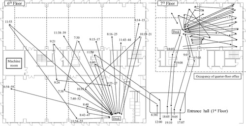
Figure 14 shows an example of occupant behavior obtained by combining the building entering and leaving model with the in-building movement model. In the figure, the movement of two occupants are tracked; the floor layout on the left shows the movements of an occupant of the sixth-floor office, while the right layout shows the movements of an occupant of a quarter-floor office on the seventh floor. Clearly, the two occupants move randomly in and out of their respective offices with different timings, and they also move randomly around their own seats. (12) $E\left(t_{sty}\right)=t_{stp}\frac{P{P}_{sty}}{1-P{P}_{sty}},$(12) (13) $P{P}_{sty}=\frac{E\left(t_{sty}\right)}{t_{stp}+E\left(t_{sty}\right)},$(13) (14) $\left[\begin{array}{c}{P}_{0,m}\\ P_{1,m}\\ P_{2,m}\\ P_{3,m}\end{array}\right]=\left[\begin{array}{c}{P}_{0,m-1}\\ P_{1,m-1}\\ P_{2,m-1}\\ P_{3,m-1}\end{array}\right]\left[\begin{array}{cccc}0.909& 0.019& 0.035& 0.037\\ 0.011& 0.909& 0.035& 0.045\\ 0.002& 0.004& 0.985& 0.009\\ 0.019& 0.037& 0.035& 0.909\end{array}\right].$(14) (15) $\left[\begin{array}{c}{P}_{0,\mathrm{\infty }}\\ P_{1,\mathrm{\infty }}\\ P_{2,\mathrm{\infty }}\\ P_{3,\mathrm{\infty }}\end{array}\right]=\left[\begin{array}{c}0.058\\ 0.102\\ 0.700\\ 0.140\end{array}\right],$(15)

Figure 14. Modeled occupant behavior.

4.2.2. Thermal sensation model

The proposed emulator applies the model developed by Takada, Matsumoto, and Matsushita (2013) to predict thermal sensation values (TSV) in a non-steady thermal environment. The regression relation used by Takada is given in Eq. 16, in which the average skin temperature T_sk [°C] and its time differential T_sk/dt [°C/s] are used as explanatory variables to evaluate the non-steady state TSV. To model individual thermal sensation, the normalized skin temperature T_sk,n, which is the difference between the actual skin temperature and the skin temperature in the thermally neutral state, T_sk,0, is used (Eq. 17). (16) $\begin{array}{rl}TSV& =a_1+a_2\left[\frac{1}{2}+\frac{\text{atan}\left(\frac{T_{sk,n}-a_3}{a_4}\right)}{\pi }\right]\\ & +a_5\left[\frac{1}{2}+\frac{\text{atan}\left(\frac{d{T}_{sk}/dt-a_6}{a_7}\right)}{\pi }\right],\end{array}$(16) (17) $T_{sk,n}\left(t\right)=T_{sk}\left(t\right)-T_{sk,0}.$(17)

The value of T_sk,n is stochastically determined from a normal distribution N(μ_sk,σ_sk²) with mean μ_sk and variance σ_sk² (Eq. 18). The predicted number of occupants who feel discomfort and complain about it is based on the TSV calculated in Eq. 16 but depends on highly subjective individual responses, coupled with the fact that some individuals will not complain, even if they experience discomfort, whereas others will complain under a slight divergence from the thermally neutral state. To account for these differences, it is assumed that the threshold of TSV for expressing dissatisfaction is stochastically determined according to the lognormal distribution LN(μ_th,σ_th²) (Eq. 19). Thus, when the TSV is lower than the threshold, dissatisfaction is considered to not occur (δ_ds= 0); when it exceeds the threshold value, dissatisfaction is expressed (δ_ds= 1). The emulator calculates the average skin temperature using a two-node model of a standard body. According to an actual survey of office buildings in Japan, conducted by Ukai and Nobe (2017a; 2017b), the clo (clothing insulation) value is in the range of approximately 0.5–1.0. Therefore, the occupant model can adjust its clo value within this range to improve the thermal sensation. (18) $T_{sk,0}=N\left({\mu }_{sk},{\sigma }_{sk}^2\right),$(18) (19) $t{h}_{tsv}=LN\left({\mu }_{th},{\sigma }_{th}^2\right)$(19) (20) ${\delta }_{ds}\left(TSV\right)=\left\{\begin{array}{ll}1& \left(|TSV|<t{h}_{tsv}\right)\\ 0& \left(t{h}_{tsv}\le |TSV|\right)\end{array}\right..$(20)

Using the above model, the individual TSV and expression of dissatisfaction by each occupant can be calculated. It is also desirable that these statistical properties can aggregate into a conventional thermal sensation model; thus, the parameters of the model are estimated so that the dissatisfaction rate calculated from a large number of occupant models matches that under the predicted percentage of dissatisfied (PPD) model by Fanger (1982). Specifically, these parameters were estimated by first calculating the results produced by the two-node model under various thermal environments and then calculating the steady-state skin temperature. Next, using Eq. 18 and Eq. 19 the thermal sensation diversity (normalized skin temperature (T_sk,n) and thresholds of dissatisfaction (th_tsv)) of 10,000 individuals were stochastically generated, and the percentage of dissatisfied occupants (PD) was calculated using Eq. 21. In addition, Eq. 22 was applied to obtain estimated parameters by applying a quasi-Newton method to minimize the error rate of PD with respect to Fanger’s PPD. The estimated parameters are shown in Table 3. (21) $PD=\frac{1}{N_{oc}}\sum _{n=1}^{N_{oc}}{\delta }_{ds,n},$(21) (22) $min\left\{\frac{|PD\left({\mu }_{sk},{\sigma }_{sk},{\mu }_{th},{\sigma }_{th}\right)-PPD|}{PPD}\right\}.$(22)

Table 3. Parameters of stochastic thermal sensation diversity model.

Parameter	μsk	σsk	μth	σth
Value	33.883	0.436	1.014	0.325

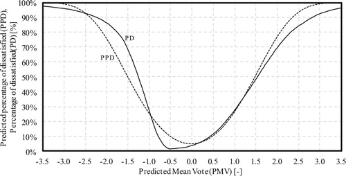
Figure 15 shows the probability densities and cumulative distribution functions of the stochastic thermal sensation diversity models constructed by applying the parameters listed in Table 3 to Eq. 18 and Eq. 19. The normalized average skin temperature falls primarily within the range 33.0–35.0°C, and the modal value of the threshold expressing dissatisfaction is approximately 0.8. The PD values obtained using these stochastic models under the thermal environment conditions, along with the corresponding PPD values, are shown in Figure 16 with the relation to the predicted mean vote (PMV). On the cold side, there is a slight error of up to 20%, where PMV takes a negative value. However, the trends in PD and PPD are consistent, with an average error of less than 5%.

Figure 15. Probability density and cumulative distribution functions of stochastic thermal sensation characteristic models.

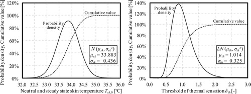
Figure 16. Relation between PMV and PPD, PD.

4.3. Simulation example

An example of a simulation using the model described in the previous section is shown. These are the operational results before the controllers are optimized.

4.3.1. Indoor thermal environment

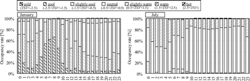
Figure 17 and Figure 18 show the monthly and hourly transition of the ratio of the thermal sensation experienced by occupants, respectively. TSV in Eq. 16 is converted into a seven-point thermal sensation scale. In the traditional simulation, a single PMV or SET* indicator is used to evaluate the average performance of the indoor thermal environment. However, in this emulator, because the thermal sensation experienced by each of the occupants is calculated, it can be evaluated as a distribution like this one. In addition, as a result of the ducting network calculations, different thermal environments are formed for each zone, and the occupants move around the zones thus exposing each occupant to different thermal environments, which enables calculating such a distribution.

Figure 17. Monthly transition of the ratio of the thermal sensation.

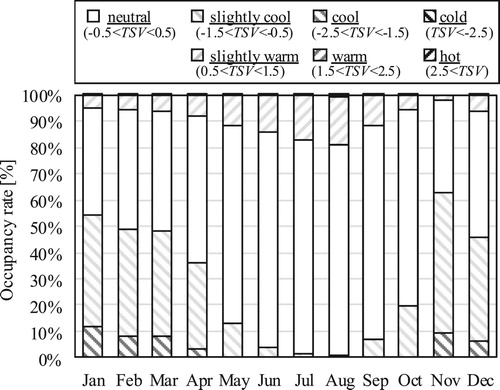
Figure 18. Hourly transition of the ratio of the thermal sensation (Winter and summer).

In this example, many occupants appear to feel cold on winter mornings. The radiation temperature in the morning is expected to be low because of the heat stored in the walls at night, so the startup time must be advanced.

Figure 19 shows an example of the distribution of indoor temperature and humidity. Only the data during the air conditioner operating time were extracted. The set point temperature is 25 °C in summer and 23 °C in winter. The on/off control for relative humidity is performed with 40 ± 10%. Unlike the traditional energy simulation, the temperature and humidity are not ideally kept at the set point but vary around the set point. This is because temperature/humidity sensors, valves, and dampers are modeled, and the quality of the feedback control is expressed.

Figure 19. Example of indoor temperature and humidity distribution.

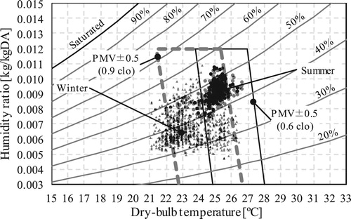
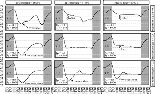
Figure 20 shows the transition of zone temperature when the PI parameters of the VAV unit are changed. The proportional gains K_P [-] are 0.1, 0.3, and 0.9, and the integration times T_I [s] are 1000, 4140, 8000 s. The air conditioner operates from 8:00–19:00. The set point temperature is 25 °C. The case in the middle (K_P = 0.3, T_I = 4140 s) is a case where the PI parameters are adjusted using the Chien–Hrones–Reswick (CHR) method (Chien, Hrones, and Reswick 1952). In this case, the temperature quickly reaches the set point after air conditioning starts. When the proportional gain is too large or the integral time is too small, overshoot occurs. On the contrary, when the proportional gain is too small or the integral time is too large, an offset remains.

Figure 20. Transition of the zone temperature when the PI parameters of the VAV unit are changed.

4.3.2. Heat source and HVAC system

Figure 21 shows the breakdown of primary energy consumption. Annual energy consumption is 403 MJ/(m²·yr), which is the general level of an office building in Tokyo, Japan. Figure 22 shows the heat production rate of heat sources. Because heat is supplied in the order of heat release from the water tank, direct-fired absorption chiller, AHP, the ratio of heat supply quantity also follows this order. To reduce the energy consumption of the absorption chiller, the operation order of the AHP should be raised, as its COP is much higher than that of the absorption chiller.

Figure 21. Breakdown of primary energy consumption.

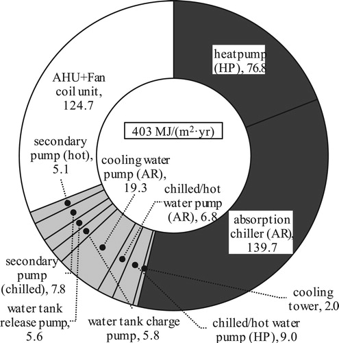
Figure 22. Heat production rate of heat sources.

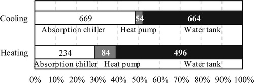
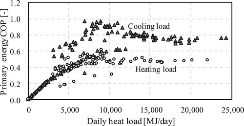
Figure 23 shows the monthly heat load and primary energy consumption. The cooling loads in April and November are extremely small, and the system COP is lowered owing to the low-partial-load operation. Figure 24 shows the relationship between the daily heat load and the primary energy COP. The COP reaches a maximum value when the daily cooling load is around 10,000 MJ/day because the outdoor air temperature is low on days when the cooling load is small, and the AHP can operate with high efficiency. However, when the heat load becomes smaller than this optimum and high efficiency point, efficiency decreases owing to the low-load operation. According to Figure 17, because many occupants feel cold in April and November, energy consumption can possibly be reduced if the low-load cooling operation is stopped, and the operation mode is changed to heating.

Figure 23. Monthly heat load and primary energy consumption.

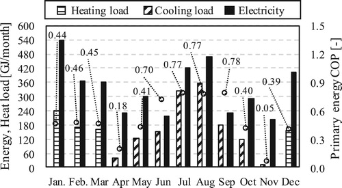
Figure 24. Daily heat load and primary energy COP.

4.4. Evaluation of energy reduction and thermal comfort

As shown in the preceding sections, differences relative to a reference building can be calculated in terms of energy consumption and comfort as ERR and DRR in Eq. 1 and Eq. 2, respectively. In this section, we consider a method for evaluating these two performance indicators as complementary relations.

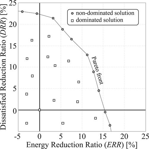
The problem of searching for an optimum point in the presence of multiple performance indicators is called the multi-objective optimization problem. According to Nguyen, Reiter, and Rigo (2014), approximately 40% of past building optimization studies applied multi-objective optimization (with the other 60% constituting single-objective studies). A typical approach to solving this problem is to apply the concept of Pareto efficiency. In general, reducing energy use and improving comfort are in a trade-off relationship in which improving one performance measure causes the other to deteriorate. This is illustrated in Figure 25, in which ERR and DRR are represented on the axes of a graph as competing performance measures. Although the combination of parameter values varies with the operation, the two are in a trade-off relationship, and a solution cannot be obtained in the upper-right quadrant, where both have high values. Thus, the possible solution combinations fall within a frontier extending from the upper left to the lower right. As the additional energy consumption required to raise comfort by one unit tends to gradually increase with the total energy consumption, the frontier is convex toward the upper right. This type of frontier is called a Pareto front, and the solutions on a curve of this type are called non-dominated solutions. A non-dominated solution is efficient because neither ERR nor DRR can be independently improved by moving away from it.

Figure 25. Application of Pareto efficiency to ERR and DRR analysis.

We changed the operation of this emulator system and tested how the evaluation value changes. Table 4 lists the changed operations, and the calculation results are shown in Figure 26.

Figure 26. Change in comfort and energy conservation by operation change.

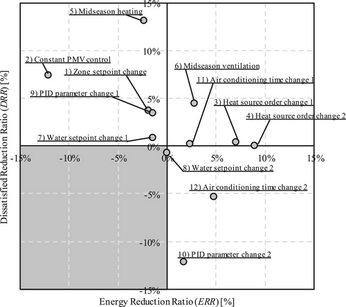
Table 4. List of changed operations.

Case	Description
1) Zone set point change	Change the set point temperature of the zone in the summer from 25.0 °C to 24.5 °C, and in the winter from 23.0 °C to 23.5 °C.
2) Constant PMV control	Using the measured dry-bulb temperature, relative humidity, and radiation temperature, calculate the set point temperature so that PMV becomes 0.
3) Heat source order change 1	Operate the AHP before the direct absorption chiller. Disable water heat storage tank.
4) Heat source order change 2	Operate the AHP sooner than the direct absorption chiller. Enable water heat storage tank.
5) Midseason heating	Change operation mode of AHU from cooling to heating in April and November.
6) Midseason ventilation	Change operation mode of AHU from cooling to ventilation in April and November.
7) Water set point change 1	Change the set point temperature of the supply water in the summer from 7.0 °C to 5.0 °C, and in the winter from 44.0 °C to 46.0 °C.
8) Water set point change 2	Change the set point temperature of the supply water in the summer from 7.0 °C to 9.0 °C, and in the winter from 44.0 °C to 42.0 °C.
9) PID parameter change 1	Change the proportional gain of the VAV PID parameter from 0.3–0.9.
10) PID parameter change 2	Change the proportional gain of the VAV PID parameter from 0.3–0.1.
11) Air conditioning time change 1	Change the operation mode of AHU after 19:00 from cooling/heating to ventilation.
12) Air conditioning time change 2	Change the operation mode of AHU after 18:00 from cooling/heating to ventilation.

Raising the temperature set point in winter and lowering it in summer will increase comfort but will also increase energy consumption (case 1). When PMV constant control is performed using the measured values of indoor air temperature and humidity and radiation temperature, comfort is further improved, but comfort improvement relative to the increase in energy consumption decreases (case 2). As pointed out in the previous section, raising the operating order of the AHP with a high COP reduces energy consumption (case 3). By increasing the rate of heat production of the AHP by using the heat storage tank, energy consumption is further reduced (case 4). Since these two cases have little influence on the indoor thermal environment, the DRR hardly changes. As shown in Figure 17, the default operation is slightly cold in April and November. If the operation during these seasons is changed from cooling to heating, energy consumption will increase, but comfort will be greatly improved (case 5). In the case of ventilation operation, although it improves comfort less than heating operation, energy consumption is also reduced (case 6). Changing the supply temperature of the chilled water and hot water has little effect on comfort and energy consumption (cases 7 and 8). When the proportional gain of the PI control of VAV is increased, comfort improves, and energy consumption increases (case 9). Although overshoot occurs, as shown in Figure 20, it may be rather cool and comfortable because the default set point temperature is high. When the proportional gain is set to 0.1, comfort is greatly reduced as the offset remains (case 10). In the default operation, heating and cooling are stopped at 22:00 at night, but if this time is changed to 19:00, energy consumption will decrease (case 11). In the evening, the radiation temperature from the wall is stable, and because there are few occupants, even with such a change in operation, the dissatisfied rate hardly increases. However, stopping cooling/heating one hour earlier at 18:00 will greatly increase the rate of dissatisfied occupants (case 12).

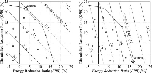
An evaluation function must be applied to select the optimal point from the set of non-dominated solutions. The simplest evaluation function is a linear combination of multiple performance indicators as given by Eq.23, in which w_ERR [0,1] is a weight factor for ERR.

An example of selecting a solution using this linear combination function is shown in Figure 27, in which the results for w_ERR = 0.5 and w_ERR = 0.8 are shown in the left and right panels, respectively. Depending on the weight factors used, different points are selected as solutions. The influence of the weighting factor is clearly significant, although the value is not always obvious. For example, research linking the quality of the indoor environment with economic value from the viewpoint of workplace productivity to enable a mutual comparison between energy and comfort is ongoing but not yet complete (Fisk and Rosenfeld 1997; Mendell et al. 2002; Nishihara, Wargocki, and Tanabe 2014). Bortoluzzi et al. (2018) reviewed the latest research results. (23) $w_{ERR}ERR+\left(1-w_{ERR}\right)DRR.$(23)

Figure 27. Examples of solutions selected using a linear combination function.

5. Discussion

In this study, a system for quantitatively evaluating building operation using an emulator was developed. Two key facets of the proposed emulator were described: 1) the communication architecture and 2) the methods used for calculating energy consumption and comfort.

The proposed emulator applies a simplified interface software architecture in which BACnet is used as the interface, thus simplifying copying and distribution and increasing the scope of application of the emulator. To this end, the function of asynchronous communication is important, and as this study showed, dividing the program into physical computation and communication control functions significantly simplifies it. Such a program structure can be easily implemented using an object-oriented language. Unlike conventional software in which these two functions are integrated, the proposed emulator must be capable of computing over a wide range of inputs. The proposed emulator also differs from conventional software in that eliminating irregular inputs in advance is difficult through filtering because the control signal can be rewritten from outside the emulator. For example, even if the operation of a refrigeration unit is suspended because of excessively high refrigerant pressure, computational processing should not be halted because of this error. As is true for real equipment, a model must be developed that outputs an error signal while continuing normal calculation.

To accurately assess the system controls, the detailed ducting and piping network must be modeled. Although the proposed emulator analytically reduces the number of unknown variables, performing the required calculations for each individual HVAC system is cumbersome, and it will therefore be necessary in the future to develop and implement an algorithm that automatically reduces the number of unknown variables that must be applied in complex networks models. Fortunately, the development of BIM in recent years has made it easier to obtain and apply digital piping and ducting route data. If such data could be automatically used in the calculation of a network model, the scenarios in which the emulator could be applied would increase significantly.

The proposed emulator models the movement and thermal sensation experienced by individual occupants. As information technology continues to develop, reflecting more individual diversity will become key to evaluating the operation of buildings. As measuring technology improves, an occupant’s position and physiological response can be more finely measured, enabling response to the wide variety of occupant demands. Studies have just begun on the use of machine learning to capture the individual diversity of occupants, and emulators can be used as testbeds to introduce these results into actual building management systems. The proposed emulator manages information on the position and thermal sensation that are not managed by the existing general real BEMS via BACnet communication.

Physically deriving an integrated evaluation index of energy performance and comfort is difficult. Further use of the emulator in actual situations should enable the generation of indicators that adopt a more practical approach based on experience. To evaluate building operation, the emulator can be applied in a number of ways. One example is using the system to certify operational performance, as an objective measure of the performance can provide useful information to an owner selecting an operation manager or building automation system. Market competition is also expected to lead to improvements in operation. Prior to completion of a large-scale real estate project, an emulator could potentially be developed and virtually operated to compare results and select an administrator. In addition, we plan to hold the WCCBO using the proposed emulator. In the WCCBO, several cyber buildings (emulator) will be uploaded to a server to compare their operation under identical conditions. Details of the competition and the source code for the emulator described in this paper can be downloaded from the following website: http://www.wccbo.org/index_en.php. This emulator is in the development stage, and its problems must be clarified by applying such competitions to improve them. We must also establish indicators that combine energy performance and comfort. The competition results will be reported in a follow-up paper.

Acknowledgements

This work was supported by JSPS KAKENHI Grant Numbers JP 16K18198 and JP 18K04462.

Additional information

Funding

This work was supported by JSPS KAKENHI Grant Numbers JP 16K18198 and JP 18K04462. Grants-in-Aid for Scientific Research (KAKENHI)

References

- American Society of Heating, Refrigerating and Air-Conditioning Engineers (ASHRAE). 2016. BACnet A Data Communication Protocol for Building Automation and Control Networks, Standard 135–2016.
- Andersen, P. D., A. Iversen, H. Madsen, and C. Rode. 2014. “Dynamic Modeling of Presence of Occupants Using Inhomogeneous Markov Chains.” Energy and Buildings 69: 213–223. doi:10.1016/j.enbuild.2013.10.001.
- Bahnke, G. D., and C. P. Howard. 1964. “The Effect of Longitudinal Heat Conduction on Periodic-Flow Heat Exchanger Performance.” Transactions of the American Society of Mechanical Engineers 86A: 105–117. doi:10.1115/1.3677551.
- Bortoluzzi, B., D. Carey, J. J. McArthur, and C. Menassa. 2018. “Measurements of Workplace Productivity in the Office Context: A Systematic Review and Current Industry Insights.” Journal of Corporate Real Estate 20 (4): 281–301. doi:10.1108/JCRE-10-2017-0033.
- Bushby, S. T., N. Castro, M. A. Galler, and C. Park. 2001. “Using the Virtual Cybernetic Building Testbed and FDD Test Shell for FDD Tool Development.” National Institute of Standard and Technology: NISTIR 6818.
- Bushby, S. T., N. M. Ferretti, M. A. Galler, and C. Park. 2010. “The Virtual Cybernetic Building Testbed – A Building Emulator.” ASHRAE Transactions 116 (1): 37–44.
- Chaudhary, G., J. New, J. Sanyal, P. Im, Z. O’Neill, and V. Garg. 2016. “Evaluation of ‘Autotune’ Calibration Against Manual Calibration of Building Energy Models.” Applied Energy 182: 115–134. doi:10.1016/j.apenergy.2016.08.073.
- Chien, K. L., J. A. Hrones, and J. B. Reswick. 1952. “On the Automatic Control of Generalized Passive Systems.” Transaction of the American Society of Mechanical Engineers 74 (2): 175–185. doi:naid/10003093715.
- Clark, D. R. 1985. “HVACSIM+ Building Systems and Equipment Simulation Program Reference Manual.” NBSIR, 84–2996.
- Coppage, J. E., and A. L. London. 1953. “The Periodic-Flow Regenerator—A Summary of Design Theory.” Transactions of the American Society of Mechanical Engineers 75: 779–787.
- DOE (Department of Energy). 2015. A Common Definition for Zero Energy Buildings. Washington, D.C.: U.S Department of Energy Office of Energy Efficiency and Renewable Energy. Accessed 1 December 2018. http://energy.gov/sites/prod/files/2015/09/f26/bto_common_definition_zero_energy_buildings_093015.pdf.
- Donald, R. B., and A. S. Howard. 1961. “A Comprehensive Approach to the Analysis of Cooling Tower Performance.” Journal of Heat Transfer 83 (3): 339–349. doi:10.1115/1.3682276.
- Dong, B., B. Andrews, K. P. Lam, M. Höynck, R. Zhang, Y. Chiou, and D. Benitez. 2010. “An Information Technology Enabled Sustainability Test-bed (ITEST) for Occupancy Detection Through an Environmental Sensing Network.” Energy and Buildings 42 (7): 1038–1046. doi:10.1016/j.enbuild.2010.01.016.
- European Parliament, Council of the European Union. 2010. Directive 2010/31/EU of the European parliament and of the council of 19 May 2010 on the energy performance of buildings, Article 9 Nearly zero-energy buildings, Official Journal of the European Union.
- Fanger, P. O. 1982. Thermal Comfort-Analysis and Applications in Environmental Engineering. Malabar, Florida: Robert E. Krieger Publishing Company.
- Fisk, W., and A. Rosenfeld. 1997. “Estimates of Improved Productivity Health From Better Indoor Environments.” Indoor Air 7 (3): 158–172. doi:10.1111/j.1600-0668.1997.t01-1-00002.x.
- Granderson, J., G. Lin, R. Singla, S. Fernandes, and S. Touzani. 2018. “Field Evaluation of Performance of HVAC Optimization System in Commercial Buildings.” Energy & Buildings 173: 577–586. doi:10.1016/j.enbuild.2018.05.048.
- Gunay, H. B., W. O’Brien, I. Beausoleil-Morrison, and J. Bursill. 2017. “Development and Implementation of a Thermostat Learning Algorithm.” Science and Technology for the Built Environment 24 (1): 43–56. doi:10.1080/23744731.2017.1328956.
- Haves, P. 1994. “Component-based modeling of VAV systems.” Proceedings of the Fourth International Conference on System Simulation in Buildings, Liège, Belgium: 31–56.
- Haves, P., A. L. Dexter, D. R. Jorgensen, K. V. Ling, and G. Geng. 1991. “Use of a Building Emulator to Evaluate Techniques for Improved Commissioning and Control of HVAC Systems.” ASHRAE Transactions 97 (1): 684–688.
- International Energy Agency (IEA). 1997. Energy Conservation in Buildings and Community Systems Programme (ECBCS). Summary of IEA Annexes 16 and 17, Annex 17 – Building Energy Management Systems (BEMS) – Evaluation and Emulation Techniques.
- International Energy Agency (IEA). 1999. Energy Conservation in Buildings and Community Systems Programme (ECBCS). Annex 25 –Real Time Simulation of HVAC Systems for Building Optimization, Fault Detection and Diagnostics.
- International Energy Agency (IEA). 2008. Worldwide Trends in Energy use and Efficiency. New Milford, Connecticut, USA: Turpin Distribution.
- International Energy Agency (IEA). 2017. Energy in Buildings and Communities Programme (ECB). IEA Annexes 60 Final Report – New Generation Computational Tools for Building & Community Energy Systems.
- International Energy Agency (IEA). 2018. Energy in Buildings and Communities Programme (ECB). IEA Annexes 66 Final Report – Definition and Simulation of Occupant Behavior in Buildings.
- International Organization for Standardization (ISO). 2003. “ISO 15099:2003 Thermal performance of windows, doors and shading devices – Detailed calculations.”.
- Japan Building Mechanical and Electrical Engineers Association (JABMEE). 1992. “HASP/ACSS/8502 Program Manual.”.
- Judkoff, R., and J. Neymark. 1995. “International Energy Agency Building Energy Simulation Test (BESTEST) and Diagnostic Method.” NREL/TP-472-6231.
- Kärki, S. H., and V. E. Lappalainen. 1994. “A new Emulator and a Method for Using it to Evaluate BEMS.” ASHRAE Transactions 100 (1): 1494–1505.
- Kays, W. M., and A. L. London. 1998. Compact Heat Exchangers. Third edition. Malabar, Florida: Krieger publishing company.
- Kelly, G. E., and W. B. May. 1990. “The Concept of an Emulator/Tester for Building Energy Management System Performance Evaluation.” ASHRAE Transactions 96 (1): 1117–1126.
- Khoury, J., Z. Alameddine, and P. Hollmuller. 2017. “Understanding and Bridging the Energy Performance gap in Building Retrofit.” Energy Procedia 122: 217–222. doi:10.1016/j.egypro.2017.07.348.
- Kim, J. B., W. Jeong, M. J. Clayton, J. S. Haberl, and W. Yan. 2015. “Developing a Physical BIM Library for Building Thermal Energy Simulation.” Automation in Construction 50: 16–28. doi:10.1016/j.autcon.2014.10.011.
- Kitano, H., T. Iwata, and K. Sagara. 2005. “Study on Mixing Model for Temperature-Stratified Thermal Storage Tank Under Variable Input Conditions in Actual Operation.” Transactions of SHASE Japan 30 (96): 31–40. doi:10.18948/shase.30.96_31.
- Langevin, J., J. Wen, and P. L. Gurian. 2015. “Simulating the Human-Building Interaction: Development and Validation of an Agent-Based Model of Office Occupant Behaviors.” Building and Environment 88: 27–45. doi:10.1016/j.buildenv.2014.11.037.
- Larech, R., P. Gruber, P. Riederer, P. Tessier, and J. C. Visier. 2002. “Development of a Testing Method for Control HVAC Systems by Emulation.” Energy and Buildings 34 (9): 909–916. doi:10.1016/S0378-7788(02)00067-1.
- Lazarova-Molnar, S., H. R. Shaker, N. Mohamed, and B. N. Jørgensen. 2016. “Fault Detection and Diagnosis for Smart Buildings: State of the Art, Trends and Challenges.” 3rd MEC International Conference on Big Data and Smart City. doi:10.1109/ICBDSC.2016.7460392.
- Lebrun, J., and S. W. Wang. 1993. “Evaluation and Emulation of Building Energy Management Systems - Synthesis Report, IEA Annex 17 Final Report”, University of Liege, Belgium.
- Matsumoto, M., and T. Nishimura. 1998. “Mersenne Twister: A 623-Dimensionally Equidistributed Uniform Pseudorandom Number Generator.” ACM Transactions on Modeling and Computer Simulation 8 (1): 3–30. doi:10.1145/272991.272995.
- Mendell, M. J., W. J. Fisk, K. Kreiss, H. Levin, D. Alexander, W. S. Cain, J. R. Girman, et al. 2002. “Improving the Health of Workers in Indoor Environments: Priority Research Needs for a National Occupational Research Agenda.” American Journal of Public Health 92 (9): 1430–1440. doi:10.2105/AJPH.92.9.1430.
- Mills, E., H. Friedman, T. Powell, N. Bourassa, D. Claridge, T. Haasl, and M. A. Piette. 2004. “The cost-effectiveness of commercial-buildings commissioning: a meta-analysis of energy and non-energy impacts in existing buildings and new construction in the United States.” LBNL – 56637, Lawrence Berkeley National Laboratory.
- Ministry of Economy, Trade and Industry (METI). 2015. Definition of ZEB and future measures proposed by the ZEB Roadmap Examination Committee. Accessed 1 December 2018. http://www.enecho.meti.go.jp/category/saving_and_new/saving/zeb_report/pdf/report_160212_en.pdf.
- Neuman, P. 2011. “Power Plant and Boiler Models for Operator Training Simulators.” IFAC Proceedings Volumes 44 (1): 8259–8264. doi:10.3182/20110828-6-IT-1002.00403.
- Neuman, P. 2012. “Power Plant and Turbo Generator Models for Engineering and Training Simulators.” IFAC Proceedings Volumes 45 (21): 313–318. doi:10.3182/20120902-4-FR-2032.00056.
- Nguyen, A., S. Reiter, and P. Rigo. 2014. “A Review on Simulation-Based Optimization Methods Applied to Building Performance Analysis.” Applied Energy 113: 1043–1058. doi:10.1016/j.apenergy.2013.08.061.
- Nishihara, N., P. Wargocki, and S. Tanabe. 2014. “Cerebral Blood Flow, Fatigue, Mental Effort, and Task Performance in Offices with two Different Pollution Loads.” Building and Environment 71: 153–164. doi:10.1016/j.buildenv.2013.09.018.
- Niwa, H., T. Watanabe, and N. Nakahara. 1995. “Study on Effects of Improper Choice of Control Parameters on the System Dynamics and Optimum Parameter Setting Methods in a VAV HVAC System.” Journal of Architecture and Planning (Transactions of AIJ) 60 (477): 19–28. doi:10.3130/aija.60.19_5.
- O’Neill, Z., and B. Eisenhower. 2013. “Leveraging the Analysis of Parametric Uncertainty for Building Energy; Model Calibration.” Building Simulation 6 (4): 365–377. doi:10.1007/s12273-013-0125-8.
- Ono, E., S. Ito, and H. Yoshida. 2017. “Development of Test Procedure for the Evaluation of Building Energy Simulation Tools.” Proceedings of the International Building Performance Simulation Association, 380–388. doi:10.26868/25222708.2017.10z.
- Page, R. L. 2000. “Brief history of flight simulation.” SimTechT 2000 Proceedings. Sydney, Australia, The SimTechT 2000 Organizing and Technical Committee.
- Pinheiro, S., R. Wimmer, J. O’Donnell, S. Muhic, V. Bazjanac, T. Maile, J. Frisch, and C. Treeck. 2018. “MVD Based Information Exchange Between BIM and Building Energy Performance Simulation.” Automation in Construction 90: 91–103. doi:10.1016/j.autcon.2018.02.009.
- Prada, A., A. Gasparella, and P. Baggio. 2018. “On the Performance of Meta-Models in Building Design Optimization.” Applied Energy 225: 814–826. doi:10.1016/j.apenergy.2018.04.129.
- Qiu, S., Z. Li, Z. Pang, W. Zhang, and Z. Li. 2018. “A Quick Auto-Calibration Approach Based on Normative Energy Models.” Energy and Buildings 172: 35–46. doi:10.1016/j.enbuild.2018.04.053.
- Serra, M., E. Franco, L. Rumi, J. M. Ferrer, and J. M. Nougués. 2017. “Web-based Operator Training System.” Computer Aided Chemical Engineering 40: 2935–2940. doi:10.1016/B978-0-444-63965-3.50491-8.
- Shaikh, P. H., N. B. M. Nor, P. Nallagownden, I. Elamvazuthi, and T. Ibrahim. 2014. “A Review on Optimized Control Systems for Building Energy and Comfort Management of Smart Sustainable Buildings.” Renewable and Sustainable Energy Reviews 34: 409–429. doi:10.1016/j.rser.2014.03.027.
- SHASE (Society of Heating, Air-Conditioning and Sanitary Engineers of Japan). 2001. “HVACSIM+(J) User manual. Type 707 PID controller (velocity algorithm).”.
- SHASE (Society of Heating, Air-Conditioning and Sanitary Engineers of Japan). 2016. “SHASE-G 1008-2016, Guideline of test procedure for the evaluation of building energy simulation tool.”.
- Takada, S., S. Matsumoto, and T. Matsushita. 2013. “Prediction of Whole-Body Thermal Sensation in the non-Steady State Based on Skin Temperature.” Building and Environment 68: 123–133. doi:10.1016/j.buildenv.2013.06.004.
- Takaguchi, H., S. Izutsu, S. Washiya, S. Kametani, H. Hanzawa, H. Yoshino, Y. Asano, et al. 2012. “Development and Analysis of DECC (Data-Base for Energy Consumption of Commercial Building).” Journal of Environmental Engineering (Transactions of AIJ 77 (678): 699–705. doi:10.3130/aije.77.699.
- Togashi, E. 2016. “The art of thermal environmental computing.” Togashi Lab. Kogakuin University, ISBN978-4990890810.
- Togashi, E. 2017. “Effect of Energy Conservation Technology on Value of Real Estate. Part 3 Development of Stochastic Office Worker Behaviour Model for Evaluating Risk of Energy Saving Investment.” Transactions of SHASE Japan 42 (240): 9–18. doi:10.18948/shase.42.240_9.
- Togashi, E. 2018a. “Risk Analysis of Energy Efficiency Investments in Buildings Using the Monte Carlo Method.” Journal of Building Performance Simulation 11. doi:10.1080/19401493.2018.1523949.
- Togashi, E. 2018b. “Development of Heat Pump Model Based on Outlet Temperature of Heat Medium.” Japan Architectural Review 1 (1): 129–139. doi:10.1002/2475-8876.1006.
- Togashi, E., and S. Tanabe. 2009. “Methodology for developing heat-load calculating class library with immutable interface.” Technical Papers of the Annual Meeting of the Society of Heating, Air-conditioning and Sanitary Engineers of Japan: 1995–1998. doi:10.18948/shasetaikai.2009.3.0_1995.
- Trčka, M., and J. L. M. Hensen. 2010. “Overview of HVAC System Simulation.” Automation in Construction 19: 93–99. doi:10.1016/j.autcon.2009.11.019.
- Tsujimoto, M., K. Sagara, and N. Nakahara. 1981. “Studies on Heat Storage Water Tank: Part 1-Experimental Study on Mixing Process of Stratified-Type Heat Storage Water Tank.” Transactions of SHASE Japan 6 (16): 23–35. doi:10.18948/shase.6.16_23.
- Udagawa, M. 1993. “Simulation of Panel Cooling Systems with Linear Subsystem Model.” ASHRAE Transactions 99 (Part 2): 534–547.
- Udagawa, M., and M. Satoh. 1997. “Energy Simulation of Residential Houses using EESLISM.” Proceedings of Sixth International IBPSA Conference: 91–98.
- Ukai, M., and T. Nobe. 2017a. “Study on Thermal Environmental Ununiformity in Office Buildings.” Journal of Environmental Engineering (Transactions of AIJ) 82 (738): 739–746. doi:10.3130/aije.82.739.
- Ukai, M., and T. Nobe. 2017b. “Consideration on Thermal Environment of Ambient Condition in Offices.” Summaries of technical papers of annual meeting Architectural Institute of Japan, 1039–1040.
- Vaezi-Nejad, H., E. Hutter, P. Haves, A. L. Dexter, G. Kelly, P. Nusgens, and S. W. Wang. 1991. “The use of building emulators to evaluate the performance of building energy management systems.” Proceedings of Building Simulation 1991 Conference. 209–213.
- Verhelst, J., H. G. Van, D. Saelens, and L. Helsen. 2017. “Model Selection for Continuous Commissioning of HVAC-System in Office Buildings.” Renewable and Sustainable Energy Reviews 76: 673–686. doi:10.1016/j.rser.2017.01.119.
- Watanabe, T., H. Niwa, Y. Nishitani, M. Zheng, M. Okumiya, and N. Nakahara. 2007. “Availability of the System Simulation for Life Cycle Management: Examination of Reproducibility and Adaptation to Fault Detection of the HVACSIM+ Dynamic Simulation Program.” Transactions of the SHASE of Japan 32 (128): 25–34. doi:10.18948/shase.32.128_25.
- Wilde, P. 2014. “The gap Between Predicted and Measured Energy Performance of Buildings: A Framework for Investigation.” Automation in Construction 41: 40–49. doi:10.1016/j.autcon.2014.02.009.
- Wimmer, R., J. Cao, P. Remmen, and T. Maile. 2015. “Implementation of Advanced BIM-Based Mapping Rules for Automated Conversions to Modelica.” Proceedings of BS2015: 14th Conference of International Building Performance Simulation Association: 7–9.
- Zheng, M., S. Hayashi, Y. Nishitani, and N. Nakahara. 1999. “A Study on Verification of the Reproducibility and Adjustment of a Parameter of Dynamic Simulation HVACSIM+(J).” Transactions of the SHASE of Japan 24 (75): 39–48. doi:10.18948/shase.24.75_39.
- Zhu, Y., H. Niwa, X. Chen, and N. Nakahara. 1994. “Study on the Dynamic Behavior and Evaluation of Energy Environment Performance in HVAC Reference System for BOFD.” Journal of Architecture and Planning (Transactions of AIJ) 59 (461): 69–79. doi:10.3130/aija.59.69_2.