Built form, urban climate and building energy modelling: case-studies in Rome and Antofagasta

Abstract

The energy performance of urban buildings is affected by multiple climate phenomena such as heat island intensity, wind flow, solar obstructions and infrared radiation exchange in urban canyons, but a modelling procedure to account for all of them in building performance simulation is still missing. This paper contributes to fill this gap by describing a chain strategy to model urban boundary conditions suitable for annual simulations using dynamic thermal simulation tools. The methodology brings together existing physical and empirical climate models and it is applied to 10 case studies in Rome (Italy) and Antofagasta (Chile). The results show that urban climate varies significantly across a city depending on the density of urban texture and its impact on the annual energy demand depends on the region's climate. The urban shadows are crucial in cooling-dominated climates (Antofagasta) while the urban heat island intensity is more important in temperate climates (Rome).

Abbreviations: ACH: Air change per hour; BPS: Building Performance Simulation; BS: British Standard; CNV: Controlled natural ventilation; H/W: height-to-width ratio of urban canyons; L/W: length-to-width ratio of urban canyons; UHI: Urban Heat Island; UWG: Urban Weather Generator model

KEYWORDS:

• Urban building energy performance
• urban weather generator
• urban morphology
• building performance simulation
• urban climate
• urban heat island

1. Introduction

Urban areas play a central role in the current environmental and climate crisis (Burdett and Sudjic 2007). According to many studies, urban environments have a negative impact on building energy performance, especially in cooling dominated climates (Crawley 2008). This is particularly important considering the huge increase in energy demand for air conditioning that is projected for the next future, due to income growth and climate change (Isaac and van Vuuren 2009; Lundgren and Kjellstrom 2013). For example, in many South and South-east Asian metropolis, the building cooling energy demand is estimated to increase by more than 40-fold in 2100 compared to 2000 (Giridharan and Emmanuel 2018).

Urban areas influence building energy performance through multiple climate and energy effects. The scarcity of green areas and water, the density of buildings and the presence of anthropogenic heat sources such as traffic and HVAC systems cause an increase of air temperature, known as the urban heat island (UHI) effect (Kolokotroni and Giridharan 2008; Palme, Carrasco, and Lobato 2016; Oke et al. 2017; Salvati, Palme, and Inostroza 2017). Furthermore, the complex geometry of the urban surface decreases the solar access of building facades (Chatzipoulka, Compagnon, and Nikolopoulou 2016), modifies the wind speed and direction (Di Bernardino et al. 2015; Nardecchia et al. 2018) and reduces the infrared radiation exchange between buildings and their surroundings (Chatzipoulka, Nikolopoulou, and Watkins 2015; Allegrini, Dorer, and Carmeliet 2016; Vallati et al. 2017).

These effects have contrasting impacts on buildings’ cooling and heating demand. Therefore, the resulting net energy impact of urban environments depends on the climate type (Palme, Inostroza, and Salvati 2018), the density of urban context (Salvati, Coch, and Morganti 2017; Salvati et al. 2019) and the function, form and construction characteristics of buildings (Futcher, Kershaw, and Mills 2013; Futcher, Mills, and Emmanuel 2018; Palme and Salvati 2018).

For these reasons, the energy performance of urban environments has gained more attention by researchers from different disciplines, so that urban building energy modelling has been recently defined a ‘nascent field’ of research (Reinhart and Cerezo Davila 2016). The studies in this field use different tools and procedures depending on the scale and objective of the analysis.

Tools and methods have been developed for estimating building energy loads at the city scale. These are normally divided into two categories: top-down and bottom-up approaches (Frayssinet et al. 2018). The top-down approach is statistically based and uses city-level or regional-level data to estimate the spatial distribution of energy consumption across a city based on macroeconomic indicators such as population density and income, energy price, urban morphology etc. The bottom-up models calculate the energy consumption at the city level starting from each individual building and can be either statistically-based or physically-based or hybrid models (Kavgic et al. 2010).

To increase the precision of bottom-up approaches, some methodologies have been proposed to include local climate in the energy performance simulations of buildings in urban contexts (Lauzet et al. 2019). However, in most of the cases, only a subset of the urban climate modifications are included in the analysis. Several studies focused on the impact of urban air temperature increase – i.e. the UHI intensity – on buildings’ energy demand, using both measured and modelled urban air temperatures to force dynamic thermal simulations. In Mediterranean cities, the UHI intensity was found to increase the sensible cooling demand of residential buildings by 12% – 74% (Salvati, Coch, and Cecere 2017; Zinzi, Carnielo, and Mattoni 2018). In tropical climates, the increase of buildings’ cooling demand due to the UHI effect is estimated to be around 8% to 10% (Chan 2011; Ignatius, Wong, and Jusuf 2016). In London, UK, the UHI intensity is estimated to increase the cooling demand of office buildings up to 25% and to decrease the heating demand up to 22% (Watkins et al. 2002).

Many studies also highlighted that the energy impact of the UHI effect varies across a city (Kolokotroni et al. 2012; Zinzi and Carnielo 2017), due to significant intra-urban air temperature variabilities determined by changes in urban fabric (Stewart and Oke 2012; Kolokotroni and Giridharan 2008; Salvati et al. 2019). A recent review reported that the energy impact of the UHI intensity may vary between 10% and 120% for cooling load increase and between 3% and 45% for heating load decrease (Li et al. 2019) due to inter-city temperature variations.

Other studies proved that there are strong interdependencies between urban morphology, urban microclimate and building energy performance (Steemers et al. 1998; Ratti, Baker, and Steemers 2005; Allegrini, Dorer, and Carmeliet 2012; Salvati, Coch, and Cecere 2015; Chatzipoulka and Nikolopoulou 2018; Palme, Inostroza, and Salvati 2018). These studies show that the UHI intensity is just one of the climate modifications induced by urban environments. In dense and compact urban textures, a prominent role is played by the shadows from surrounding buildings, which determine substantial variations of the cooling demand of both residential and office buildings (Salvati, Coch, and Morganti 2017; Futcher, Mills, and Emmanuel 2018; Palme, Inostroza, and Salvati 2018).

Some studies focused on the infrared radiation exchange in urban environments, showing that low sky view factors and higher surface temperatures cause a further increase in the cooling demand of urban buildings (Allegrini, Dorer, and Carmeliet 2012; Vallati et al. 2017; Palme and Salvati 2018).

Other studies highlighted that the potential for night cooling ventilation is strongly reduced in urban areas due to higher air temperatures and reduced wind speeds in urban canyons (Kolokotroni, Giannitsaris, and Watkins 2006). However, the canyon effect on wind flow was also found to reduce buildings’ heating demands, due to the impact on pressure coefficients and thus infiltration and air change rates (Georgakis and Santamouris 2006; Khoshdel et al. 2017).

Considering these results, all the climate modifications determined by an urban context should be accounted for when performing building performance simulations (BPS). Since these take place at different scales, different tools and methodologies are necessary to model their overall impact on building energy performance (Palme and Salvati 2018). To this purpose, some coupling techniques between building energy models and microclimate CFD models have been proposed (Yang et al. 2012; Lauzet et al. 2017, 2019). However, these have some limitations, including the need of expert knowledge of CFD simulation and coupling techniques, an increase in simulation costs and a very high computational time (which only allows simulation of short periods, usually few days). A modelling methodology to account for all the urban microclimate modifications in the estimation of the annual energy demand of buildings in urban context is still missing.

To fill this gap, this paper proposes a chain strategy to model urban boundary conditions suitable for annual simulations using dynamic thermal simulation tools. The proposed methodology brings together a set of physical and empirical models to calculate the air temperature, wind speed, solar access and surface temperature modifications determined by an urban context. The methodology is conceived for urban canyons with high height-to-width ratios and it is designed to generate climate outputs that are compatible with commonly used dynamic thermal simulation tools; in this paper TRNSYS is used.

The paper is structured as described in the follow: Section 2 describes the models used to calculate the urban climate outputs and the steps to use them as input to TRNSYS calculations. Section 3 describes the application of the modelling methodology to ten urban textures of Rome and Antofagasta used as case studies. Section 4 presents the results of the case studies, which include the urban climate modifications determined by built form and their impact on buildings’ energy performance (i.e. cooling, heating and annual demand). Section 5 discusses the results highlighting the variation of the net energy impact of built form depending on the climate type and density of urban texture.

2. Materials and methods

The modelling methodology proposed in this study uses validated models to define the microclimate conditions of an urban context to be used as inputs to BPS with TRNSYS v17. The modelling chain procedure is outlined in Section 2.1, where the proposed models are introduced. The models are then described in more detail in Sections 2.2–2.6.

2.1. Modelling chain procedure

The proposed modelling chain procedure consists of two phases (Figure 1). First, the urban geometry parameters required in the climate calculations are computed. These are used to model the climate variables of urban textures, namely air temperature, relative humidity, surfaces’ temperature, obstruction angles on facades and urban wind speed. Following that, the modelled outputs are linked to TRNSYS calculations in three different ways: (1) by using modified weather files, (2) by defining shadow masks for the building surfaces and (3) by linking spreadsheet files in the corresponding TRNSYS type (i.e. the hourly urban surface temperature for long wave radiation exchange and the apartment air change per hour due to wind-driven ventilation).

Figure 1. Scheme of the chain modelling strategy.

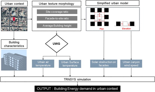
The urban air temperature, relative humidity and surface temperature of surrounding buildings are generated by the Urban Weather Generator model (Bueno, Norford, et al. 2013; Mao et al. 2017, 2018), version V4.

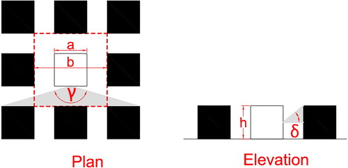
The solar obstruction on facades is computed on simplified geometrical models of the urban area using the horizontal and vertical solar obstruction angles (Figure 2).

Figure 2. Simplified geometrical model for the calculation of the horizontal (γ) and vertical (δ) obstruction angles.

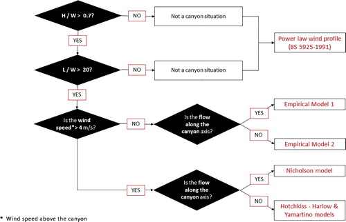
The wind speed attenuation in urban canyons is calculated considering the higher roughness of the urban area and the canyon effect. The calculations are based on empirical models, which apply to different urban situations depending on the geometry and orientation of the canyon and the wind speed and direction at the meteorological station (Figure 3).

Figure 3. Algorithm for the calculation of wind speed in urban canyon, modified from (Ghiaus et al. 2004).

2.2. Urban air temperatures and surface temperatures with UWG

The urban air temperatures and surface temperatures of walls and roads are calculated using the MATLAB version of UWG V4.¹ UWG generates urban weather files from hourly weather data measured at operational weather stations. The urban weather file has modified values of air temperature and humidity to capture the local heat island intensity of an urban area (Bueno, Norford, et al. 2013).

UWG is an urban canopy model including a building energy model. UWG uses several input parameters for the calculation of the neighbourhood-scale UHI intensity. Among these, the urban morphology parameters have been found to be crucial to the UHI intensity estimation (Nakano et al. 2015; Palme, Carrasco, and Lobato 2016; Salvati, Coch, and Cecere 2016; Mao et al. 2017; Salvati et al. 2019). Three urban morphology parameters are used to characterize an urban context:

• Site coverage ratio (ρ): ratio of the building footprints area to the urban site area

• Facade-to-site ratio (VH): ratio of the building facades area to the urban site area

• Average building height (H): average height of building normalized by building footprint

Based on these, UWG calculates the average width and height of urban canyons in the area.

An advantage of UWG compared to CFD models is that it takes into account the anthropogenic heat released into the atmosphere by buildings and traffic. The daily profile of the sensible heat due to traffic is set as an input parameter, while the waste heat from buildings’ HVAC system is calculated as proportional to the energy consumption of each building type in the area (i.e. residential, commercial, offices etc.).

The surface temperature and air temperature calculated by UWG are based on an Urban Canopy and Building Energy Model described in detail in the reference publications by Bueno and Mao (Bueno et al. 2011; Bueno, Hidalgo, et al. 2013; Bueno, Norford, et al. 2013; Mao et al. 2017). The canyon air temperature accounts for the heat fluxes from walls, windows and the road and the anthropogenic heat fluxes due to exfiltration and waste heat from building HVAC systems and traffic. The external surface temperatures of walls and roads are calculated based on the building energy balance, the incoming solar radiation – calculated assuming and average canyon orientation – and the longwave radiation among walls, road and the sky.

2.3. Solar obstructions on building facades

The average solar access of building facades is calculated on simplified geometrical models of urban textures. The simplified models consist of square-plan buildings arranged on an orthogonal street network and have the same average density of the real urban textures, namely the same values of the morphology parameters (ρ, VH, H). The size of the buildings and the distance between them (a and b in Figure 2) are calculated based on the following equations (Masson 2000; Bueno, Norford, et al. 2013): (1) $\begin{array}{rl}\rho & =\frac{a^2}{{\left(\frac{a}{2}+\frac{b}{2}\right)}^2}\end{array}$(1) (2) $\begin{array}{rl}VH& =\frac{4a\times H}{{\left(\frac{a}{2}+\frac{b}{2}\right)}^2}\end{array}$(2)

Each urban context is thus transformed in a representative morphological environment whose values of a, b, and H give the same site coverage ratio and facade-to-site ratio of the real urban texture. The simulated building is assumed to be in the centre of the representative morphological environment and the horizontal and vertical obstruction angles γ and δ are calculated in the middle of each floor, as represented in Figure 2. The angles γ and δ are used to define the shadow masks of the transparent and the opaque surfaces in the TRNSYS models. The shadow masks can be defined in TRNSYS with a desired angular step of description.

2.4. Long wave exchanges

In TRNSYS 17, the infrared radiation exchange between surfaces is calculated considering the temperature of the building walls and two fictive temperatures, namely the fictive sky temperature (obtained as a function of sky cloudiness) and another temperature for the opposite surface with respect to the sky.

For an urban context, we defined this second temperature as the Urban Surface temperature $\left(T_{UrbSurf}\right)$ calculated by Equation (5): (3) $T_{UrbSurf}=\frac{V{F}_w\times T_{\text{wall}}+V{F}_R\times T_{\text{road}}}{\left(V{F}_w+V{F}_R\right)}$(3) Where T_wall and T_road are the surface temperature of walls and roads calculated by UWG, VF_w is the view factor between the building facade and the surrounding buildings’ facades and VF_road is the view factor between the building facade and the road. The view factors are calculated on the simplified models for each floor and used in TRNSYS for the infrared radiation exchange of the external surfaces of the building. The $T_{UrbSurf}$ is used for the long-wave radiation exchange between the building facades and the surrounding urban environment, while the fictive sky temperature is used for the long-wave radiation exchange with the sky, proportionally to the facade’ sky view factor.

2.5. Urban wind speed

The wind speed in urban environment is calculated from the undisturbed wind speed by applying different models and attenuation coefficients according to the location of the area within the city and the urban canyon geometry and orientation with respect to the undisturbed wind direction.

The calculation methodology is based on the models proposed by the European project URBVENT (Ghiaus et al. 2004) with few modifications (Figure 3). This approach allows the generation of hourly annual data to substitute the undisturbed wind speed data in the weather files used in BPS.² Different calculation methods are applied depending on the urban canyon geometry and the undisturbed wind speed above the canyon. The first method applies to canyons with low height-to-width (H/W) ratios or length-to-width (L/W) ratios. The second method applies to deep canyons (i.e. with H/W ratio higher than 0.7) and wind speed above the canyon higher than 4 m/s and the third method applies to deep canyons with wind speed above the canyon lower than 4 m/s.

(1) Canyon/not canyon situation

The first check for urban wind speed calculation is to verify whether there is a canyon situation or not. Two conditions determine a canyon situation: (i) the ratio of the height of the buildings to the width of the street – or the canyon aspect ratio H/W – is more than 0.7 and (ii) the ratio of the street length – distance between main intersections – to the street width is less than 20. These thresholds values identify the starting of the skimming flow according to Oke (1988), namely when the bulk of the flow above the building arrays does not enter the canyon. When the canyon H/W ratio is below 0.7, there is a wake-interference flow or isolated obstacle regime for low ratios.

Urban areas without canyon situations can be low-density developments or small-grain urban structures where the presence of many crossroads at short distance cancel the canyon effect. In these situations, the URBVENT suggested a rule of thumb, namely a terrain correcting factor to modify the undisturbed wind speed values (Ghiaus et al. 2004, 60).

In this study, instead, the urban wind speed in these situations is calculated using the power law as included in the current British Standard (BS) (British Standards Institution 1991) for natural ventilation design. The power law expression is based on wind measurements in urban canyons and open sites in the UK over the period 1965–73 (Caton 1977). It allows the calculation of the hourly wind speed at a datum height from the undisturbed wind speed at the meteorological station, considering the roughness of different types of terrain, including urban areas, using Equation (6): (4) $\frac{V}{V_m}=k{Z}^{\mathit{\alpha }}$(4)

Where Z is the datum height (m), V is the mean wind speed at datum height (m/s), $V_m$ is the mean wind speed at the meteorological station (m/s), k and α are coefficients that depend on the terrain roughness reported in Table 1. For a ‘not canyon situation’, the ‘urban’ coefficients reported in Table 1 are used.

Table 1. Terrain coefficients for use with Equation 4 (British Standards Institution 1991).

Terrain Coefficient	k	α
Open, flat	0.68	0.17
Country with scattered wind breaks	0.52	0.20
Urban	0.35	0.25
City	0.21	0.33

(2) Canyon situation and wind speed lower than 4 m/s:

When a canyon exists and the wind speed above the canyon is low, the air circulation is mainly triggered by thermal phenomena, but no coupling is established between the flow on top of the buildings and the flow within the canyon. The wind speed above the canyon is calculated from the undisturbed values applying expression (6) for Z equal to 1.2 H.

The threshold value to establish the coupling varies from about 2 m/s for canyons with H/W ratios of about 1 (Nakamura and Oke 1988) to higher wind speed of about 4–5 m/s for canyons with higher aspect ratios (Santamouris, Georgakis, and Niachou 2008). In these situations, the airflow within the canyon is scattered and characterized by significant fluctuations that are very difficult to predict. Studies showed that the mean wind speed can be predicted with sufficient accuracy using data-driven models, such as the model proposed by Santamouris, Georgakis, and Niachou (2008) and used in this study. The model was developed based on an extensive experimental campaign in different canyons in Athens in 2001. The values of the more probable wind speed in deep urban canyons as a function of the prevailing thermal and inertia phenomena are presented in Tables 2 and 3. The flow is considered parallel if the wind direction is within ±20 degrees with respect to the canyon axis. For perpendicular or oblique flows, different values correspond to the windward and leeward facades; the average value is assumed as the mean canyon wind speed in this work.

Table 2. Empirical Model 1. Z is the datum height (m) and H is the height of the canyon (m).

Empirical model 1 (Parallel flow):
If: Z/H > 0.5	0.75* V(H) m/s
Z/H < 0.5	0.5 m/s

Table 3. Empirical Model 2. Z is the datum height (m), W is the width of the canyon (m), V_m is the meteorological station wind speed (m/s) and H is the height of the canyon (m).

Empirical Model 2(flow not parallel):	Near WINDWARD facade	Near LEEWARD facade
IF Z/W < 1.5	0.5 m/s	50% of the value calculated close to the windward facade
IF Z/W > 1.5 AND Vm < 2 m/s	1 m/s	50% of the value calculated close to the windward facade
IF Z/W > 1.5 AND Vm > 2 m/s	0.75 * V(H) m/s	50% of the value calculated close to the windward facade

It has to be highlighted that this methodology can be considered valid within the limits of the experiment reported by the authors, namely aspect ratios between 1.7 and 3.25. This means that it is suitable for deep canyons located in regions that have similar solar irradiation compared to Athens.

1. Canyon situation and wind speed greater than 4 m/s:

When the wind speed above the canyon is greater than 4 m/s, coupling is established between the flow on top of the buildings and within the canyon. In this case, the canyon wind speed is calculated using the Nicholson model for parallel flows and the Yamartino's and Hotchkiss & Harlow models (Hotchkiss and Harlow 1973; Yamartino and Wiegand 1986) for perpendicular or oblique flows. This methodology was validated by Georgakis and Santamouris with numerical simulations (Georgakis and Santamouris 2008).

For parallel flows, the canyon wind speed profile is calculated according to expressions (7) (Nicholson 1975; Georgakis and Santamouris 2008): (5) $V_{urb}=U_0\exp \frac{Z}{Z_2}$(5) Where Z is the datum height from ground in which wind speed is calculated, U₀ is the canyon wind speed at Z = 0 and Z₂ is the roughness length for the obstructed sub-layer calculated with expression (8): (6) $Z_2=0.1\frac{H^2}{Z_0}$(6) Where Z₀ is the aerodynamic roughness length of the area (reference values in Table 4) and H is the average buildings height. The value of U₀ for expression (7) is derived by using expression (9) (Nicholson 1975): (7) $V_H=U_0{e}^{\frac{H}{Z_0}}$(7) Where V_H is the wind speed at the building height, calculated with the power law.

Table 4. Typical roughness length values Z_o, for urbanized terrain.

Terrain type	Z0 (m)
Scattered Settlement (farms, villages, trees, hedges)	0.2–0.6
Suburban:
Low density residences and gardens	0.4–1.2
High Density	0.8–1.8
Urban:
High Density, < 5 story row and block buildings	1.5–2.5
Urban high density plus multi-story blocks	2.5–10

The expression (7) is valid to calculate wind speed within the canyon when the coupling is established and the wind flow is parallel to the canyon axis; the power law reported in expression (6) is applied instead when the calculation height (Z) is higher than the average building height.

When the coupling is established (for wind speed higher than 4 m/s in deep canyons) and the flow is not parallel, cross-canyon vortices or helical flow are generated along the canyon. In this case, the total wind speed inside the canyon is calculated as the resulting of the along canyon-axis component $\left(u\right)$, the cross canyon axis component $\left(v\right)$ and the vertical component $\left(w\right)$ as proposed and validated by Georgakis and Santamouris (2008), namely: (8) $W_t=\sqrt{W_h^2+w^2}$(8) Where $W_t$ is the total wind speed in the canyon and $W_h$ the air velocity inside the canyon at horizontal level given by expression (10): (9) $W_h=\sqrt{u^2+v^2}$(9)

The vertical $\left(w\right)$ and cross canyon-axis $\left(v\right)$ components are calculated according to Hotchkiss and Harlow (1973) with expressions (11) and (12): (10) $\begin{array}{rl}v& =\frac{A}{K}\left[e^{ky}\left(1+ky\right)-\text{β}{e}^{-Ky}\left(1-ky\right)\right]\sin \left(kx\right)\end{array}$(10) (11) $\begin{array}{rl}w& =-Ay\left(e^{ky}-\text{β}{e}^{-ky}\right)\cos kx\end{array}$(11)

Where:

1. K = π/W, with W the canyon width

2. β = exp (−2KH), with H the canyon height

3. A = kV_H/(1 – β), with V_H the wind speed at the point W/2, Z = H

4. Y = Z–H, where Z is the height from the ground in which we want to calculate urban canyon wind speed.

The along canyon-axis $\left(u\right)$ is calculated with Yamartino and Wiegand model (1986) with expression (13). (12) $u=V_H\text{ log}\left[\left(z+z_0\right)/z_0\right]/\text{log}\left[\left(H+z_0\right)/z_0\right]$(12)

2.6. Wind-inducted building air change rate methodology

The decrease of natural ventilation potential in urban environments is considered in the modelling methodology by setting the air change per hour (ACH) of each space in the building as a function of the urban wind speed.

The ACHs values are defined dividing the hourly airflow rates [m³/h] by the built volume [m³], assuming a net floor height of 2.7 m. The hourly airflow rates are calculated according to expression (12), considering the flowrates(average hourly values) induced by wind forces on the considered openings – see also (Allard 1998; Grosso 2017) and the method described in (Chiesa and Grosso 2017b): (13) $q_v=v_{\left(w\right)}\sqrt{\frac{|c_p^{+}-c_p^{-}|}{\frac{1}{C_{d_1}^2+A_1^2}+\frac{1}{C_{d_2}^2+A_2^2}+\dots \frac{1}{C_{d_n}^2+A_n^2}}}$(13) Where $v_{\left(w\right)}$ is the hourly wind velocity at the window height, $c_p^{+}$ and $c_p^{-}$ are the pressure coefficients of the considered openings, c_d is the opening discharge coefficient here assumed as 0.6 (Chiesa and Grosso 2017a), A is the net opening area and the subscript numbers are the progressive opening distribution between inlet and outlet one. In the case-study analysis (Section 3), all the openings on the same facade are considered together as one single inlet or outlet window/grid, to be in accordance with the geometry of the TRNSYS models.

The hourly wind velocities for the estimation of the ACH values are calculated for each location and floor height using the models described in Section 2.5.

The pressure coefficients (C_p) are defined according to the simplified-parametric-model approach described in Grosso (2017); this method considers the geometric ratio of the building and the incident angle of wind to determine the coefficients values on each facade. The mentioned approach combines tabular data (building size ratios) and parametric-equations (wind incident angles) to provide an average pressure coefficient for each facade. For each hour, the average C_p value for each facade is calculated and used to populate expression (12) and the difference between the C_p values of adjacent facades is defined for each space.

As a general assumption, the tabular and parametric-equation methods for C_p calculation are considered more suitable for small buildings, with a limited number of floors and with openings located in the central part of the facades. On the other hand, when CFD values are not available, the pressure coefficients for BPS are normally calculated using similar methods to the one adopted in this study, i.e. tabular, parametric and database values. CFD calculations and wind tunnel experiments can provide a much more accurate distribution of the pressure coefficients over building facades. Nevertheless, these two approaches are costly, require a significant computation/analysis time and specific expertise and instruments that are not common among practitioners. Parametric regression-based models such as the one proposed by Swami and Chandra (1987) are more suitable for architectural design. However, this method is not able to estimate the vertical or horizontal distribution of coefficients and it does not consider urban context parameters such as area density or surrounding building heights. Only very few tools are able to calculate the distribution of pressure coefficients on facades (Costola, Blocken, and Hensen 2009); these are the Cp generator (TNO) (Knoll, Phaff, and de Gids 1995) and the CpCalc+ tool (Grosso 1992), which is also used in ESPr – see also (Ramponi, Angelotti, and Blocken 2014).

Considering the aim of the proposed methodology and in accordance with several other studies (i.e. AIVC tables), we adopted the tabular approach for the case studies analysed in this paper (Section 3), considering the hourly values of wind direction and incident angles on facades.

A further modelling assumption is that the share of windows area devoted to CNV (Controlled Natural Ventilation) is 50%. This is a typical assumption in the CNV design of residential buildings for either manually or activated (e.g. by linear actuators) windows opening for natural ventilation of spaces. The CNV-devoted window type is supposed to be awning type (net opening area equal to 30%), being a frequently adopted solution thanks to high controllability levels, rain protection, security by intrusions, and low draft risk (Holzer and Psomas 2018).

In the TRNSYS models, the windows are placed only on the main facade and the cross ventilation effect is generated by opposite windows and devoted grids positioned on the adjacent walls.

3. Case study analysis

The aim of the case study analysis is to investigate the variability of urban microclimate conditions determined by different built forms across a city and the relative energy impact on buildings’ energy demand in different climate regions. The modelling chain procedure described in Section 2 is thus applied to analyse the energy demand of residential buildings located in five urban textures of Rome, Italy (Mediterranean climate) and Antofagasta, Chile (Subtropical Desert Climate).

3.1. Building performance simulation (BPS) workflow

The annual energy demand of two building typologies was simulated in open-rural conditions and in the five urban textures of each city.

The annual energy demand of the two building typologies in open-rural conditions are simulated without considering any urban effect and using the typical weather files used for building energy simulations for each city. After that, urban simulations are performed for the same typologies using the microclimate boundary conditions corresponding to the different urban textures. The urban simulations are performed in sequence by including one climate modification at the time in order to evaluate their relative impact on the buildings’ energy demand. The different climate modifications were added in the following order:

1. shadow masks to account for solar obstructions on facades

2. UWG weather files with urban air temperature and relative humidity

3. urban surface temperatures and view factors for infrared exchange

4. ACH determined by the urban wind speed in each urban texture

3.2. Urban textures analysed

The five urban textures examined for each city represent a sample of urban densities which have different impacts on the local urban climate. Table 5 presents the values of the urban parameters used in the calculation of the urban wind speed and UHI intensity. These have been computed over an area of about 250 m length, as suggested for local urban climate studies (Stewart and Oke 2012; Salvati, Coch, and Cecere 2016).

Table 5. Urban parameters of the 10 urban textures of Rome and Antofagasta.

urban Area	Terrain Type	Z0 -Roughness length urbanized terrain	Site coverage ratio	Facade-to-site ratio	Average Building height	Ratio of Building Length to street width > 20
Rome
Campo Marzio	City	2.5	0.79	1.77	17.34	YES
Centocelle	Urban	1.1	0.34	1.35	14.70	NO
Tridente	City	2.5	0.70	1.96	16.50	YES
Don Bosco	Urban	2.5	0.43	1.68	25.50	YES
Prati	Urban	2.5	0.49	1.43	19.50	YES
Antofagasta
Corvallis	Urban	0.8	0.30	0.38	2.96	YES
Coviefi	City	2.5	0.75	1.47	11.56	YES
Jardines Sur	Urban	1	0.68	0.97	4.02	YES
Centro	Urban	2	0.77	1.83	11.11	YES
Brasil	City	3	0.42	2.06	20.53	YES

The vegetation coverage and anthropogenic heat from buildings and traffic are also important parameters for the UHI calculation by UWG. The vegetation coverage was set to 10% in Rome and 0% in Antofagasta, as indicated by previous studies (Palme, Inostroza, and Salvati 2018; Salvati et al. 2019). The case studies in Rome differ in terms of building typology mix; two of them, Campo Marzio and Tridente, are characterized by a mix of residential, commercial, hotel and office buildings while the other three are residential neighbourhoods. This was included in the UHI estimation by providing the percentage of each building typology, which is used by UWG to calculate the waste heat from HVAC systems. The anthropogenic heat from traffic was also included, considering a two-peak daily profile, with the same peak value equal to 25 W/m² in all cases.

3.3. Building typologies characteristics

Two building typologies are simulated: detached houses and apartment blocks. These differ for number of floors and ratio of windows-to-wall but have the same U-values for the envelope, as presented in Table 6.

Table 6. Envelope parameters used in BPS for each building typology.

	U-values [W/m^2K]
BUILDING TYPOLOGY	Wall	Window	Roof	Infiltration [ACH]	Windows to wall ratio [%]	No. of floors
DT: Detached House	2.16	5.8	0.57	0.2	13% main facade	2
					6% opposite facade
					0% other facades
AP: Apartment Block	2.16	5.8	0.57	0.2	25% main facades	5
					3% other facades

In Antofagasta and in northern Chile in general, the common construction system is reinforced concrete, without insulation, with U-values in the range of 3–4 W/m²K. Roofs are normally insulated with 40 mm of polystyrene or rock wool, with U-values of 0.8–0.9 W/m²K. Windows are single-glazed, with aluminium frame, with typical value of 5.8 W/m²K. Thermal codes are evolving in the country and limiting values will be probably introduced in the future.

In Rome, most buildings were built before the introduction of the first building regulations on energy efficiency (law number 373 in 1976 and law number 10 in 1991) and thus present high transmittance values on average. Two of the case studies (Tridente and Campo Marzio) belong to the city’ historic centre where the typical construction system is solid stone walls, with average U-values around 2 W/m²K or even higher. The other case studies are developments of the 80’s and 90’s, characterized by cavity walls constructions with no or very little insulation. In most of the buildings, single glazed windows are still used. The last building regulation on energy efficiency mandates much higher performance for the building envelope, with U-values below 0.34 W/m²K in Rome. In this study we used U-values that are representative of most of the existing building stock of the two cities.

Table 7 presents the HVAC and occupancy input parameters used in the BPS for both cities. The fixed infiltration rate ensures a minimum ACH for indoor air quality. For the calculation of natural ventilation, windows are assumed to be open if the external temperature is in the range 20–26°C, otherwise the wind-induced ACH are considered negligible. The outdoor air temperature range is set to avoid undesired ventilation heat losses during winter and mid seasons or heat gains in summer when cooling is on. It should be noted that air temperatures higher than 26 degrees (but lower than 29–30) could increase thermal comfort in free running buildings, due to the effect of the air speed on the human body. However, this study is focused on building energy use and a fixed set point (26 °C) is set for the cooling demand calculation; for this reason, windows are considered closed when the outdoor air temperature is higher than 26°C.

Table 7. Occupancy and HVAC parameters used in BPS.

Solar protection	Cooling set-point & Schedule	Heating set point & Schedule	Lighting schedule	Occupancy
0.7 if solar radiation on window > 140 W/m^2	26°C	18 (15) °C	6–22	0–24
0 if solar radiation on window < 120 W/m^2	ON: 0–24	ON: 6–22

4. Results

Figure 4 presents a comparison of the climate in Rome and Antofagasta.

Figure 4. Comparison of the average daily cycle of air temperature, wind speed and solar radiation for the warmest and coldest month of the year in Rome (August and January) and Antofagasta (January and July). The values are averaged over the number of days of each month.

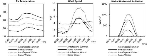
The Köppen-Geiger climate classification for the two cities is Csa Mediterranean climate for Rome and Bwk Subtropical Desert Climate for Antofagasta. Rome has a high daily and annual range of air temperature, with much higher summer temperatures and much lower winter temperatures compared to Antofagasta. On the other hand, solar radiation is higher in Antofagasta than in Rome throughout the year. The daily variation of wind speed shows the influence of the ocean in Antofagasta and also the impact of the sea breeze in summer in Rome.

Due to these differences, the urban microclimate modifications and the consequent energy impact on buildings are expected to be different in Rome and Antofagasta.

4.1. Boundary microclimate conditions corresponding to different urban textures

The average urban microclimatic conditions generated by the selected morphologies in the hottest month of the year are shown in Figures 5 and 6 for Rome and Antofagasta respectively.

Figure 5. Microclimate modifications determined by urban form in the 5 case studies of Rome. The climate variables are the daily means in the hottest month (August).

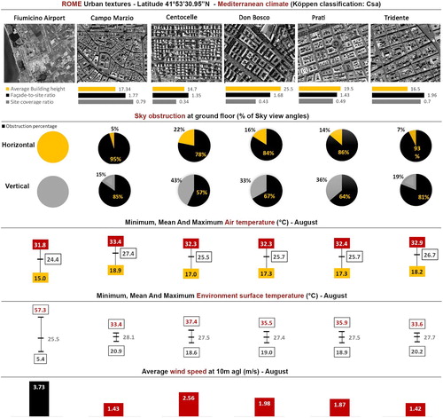
Figure 6. Microclimate modifications determined by urban form in the 5 case studies of Antofagasta. The climate variables are the daily means in the hottest month (January).

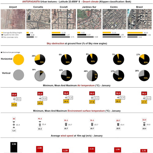
The night-time heat island intensity is similar in the two cities, varying between +3.9°C (Campo Marzio) and +2°C (Centocelle) in Rome and +3.5°C (Centro) and +1.6°C (Corvallis) in Antofagasta. Compared to Antofagasta, Rome shows a higher increase in the mean and maximum urban temperatures, which is probably the consequence of the higher diurnal variation of air temperature in Rome (around 17°C) compared to Antofagasta (around 10°C). The texture of Campo Marzio in Rome shows the highest temperature increase throughout the day, equal to +1.6°C on the maximum, +3.0°C on the mean and + 3.9°C on the minimum temperature compared to the airport station. In Antofagasta, the hottest urban texture is Centro, with an increase of +1.3°C on the maximum, +1.4°C on the mean and +3.5°C on the minimum temperature with respect to the airport station.

The results reported in Figures 5 and 6 also show that the daily surface temperature range is reduced in both cities compared to the corresponding rural-open environment, with a decrease in the maximum temperatures due to urban shadows and an increase of the minimum temperatures, due to the low urban sky view factors. The texture Corvallis in Antofagasta shows a higher maximum surface temperature (41.1 °C) compared to the other case studies (about 30 °C); this is probably due to the low average building height (less that 3 m) of the area, which reduces the beneficial effect of building shading during day time.

The average buildings height is also strongly related to the vertical obstruction angle β and thus the solar obstructions on facades. For similar values of the Site coverage ratio (ρ) – or urban compactness – the sky view factor of building facades decreases significantly with an increase in the average buildings height. This is clear comparing the vertical obstruction percentages of Centocelle, Rome (ρ = 0.34, H = 14.7 m) with the ones in Corvallis, Antofagasta (ρ = 0.30, H = 2.96).

The average wind speed in the urban textures compared to the undisturbed flow is reduced by 38–68% in Rome and by 35–63% in Antofagasta, depending on the location, morphology and orientation of the urban texture.

4.2. Impacts of the urban microclimates on building energy demand

Figures 7 and 8 show the building cooling demand for each typology in a rural-open environment and in the analysed urban textures of Rome and Antofagasta.

Figure 7. Building cooling demand without urban context and within the selected urban textures of Rome.

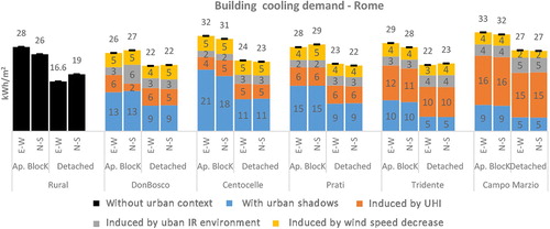
Figure 8. Building cooling demand without urban context and within the selected urban textures of Antofagasta.

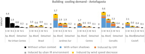
Figure 9. Annual heating and cooling demands per square metres for each typology in the urban textures of Rome. The average values of the E-W and the N-S orientation are reported.

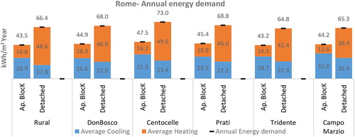
The stacked bars indicate the energy impact of each microclimate modification; the blue bars represent the reduction of the cooling demand in urban textures due to urban shadows compared to the open-rural one (black bars). The other colours show the cooling increase determined by the UHI intensity, the infrared radiation exchange and the wind speed reduction in the urban textures.

The order of the simulations allowed to highlight the opposing energy outcome of urban shadows compared to the other urban microclimate modifications. The shadows in an urban context reduce cooling demand, while all the other modifications cause an increase. Therefore, the net energy impact of urban context can be positive or negative depending on the urban context and climatic conditions.

The results indicate that in Antofagasta, where summer temperatures are lower than in Rome, the net increase in cooling demand due to UHI intensity is lower than the decrease determined by urban shadows, resulting in a net reduction of the cooling demand in three of the urban textures. In this context, the wind speed reduction plays a decisive role in determining the final building cooling demand.

In Rome, the impact of urban shadows and UHI intensity on cooling demand is similar in magnitude and opposite in contribution (positive the first and negative the latter); therefore, the two effects tend to balance out in most of the cases. However, the ventilation reduction and the urban infrared environment determine a further increase in cooling demand, which results in a net cooling increase in most of the urban textures compared to the rural-open environment. Among the case studies, only the East–West apartment block in Don Bosco showed a net reduction in the cooling demand, while all the other cases showed an increase varying between 5% and 26% for the apartment blocks and 16% and 63% for the detached house (Table 8).

Table 8. Relative variation of the building heating (H) and cooling (H) energy needs determined by the different urban textures in Rome.

		Rural		DonBosco		Centocelle		Prati		Tridente		Campo Marzio
Rome		H	C	H	C	H	C	H	C	H	C	H	C
Apartment Block	E-W	17.8	28.1	5%	−7%	−4%	13%	−2%	0%	−19%	5%	−35%	17%
	N-S	15.4	25.7	17%	5%	−1%	20%	7%	13%	−6%	9%	−25%	26%
Detached House	E-W	51.2	16.6	−7%	31%	−3%	42%	−9%	36%	−24%	33%	−33%	63%
	N-S	46.0	19.0	−3%	16%	8%	22%	2%	15%	0%	19%	−8%	41%

The impact of urban climate on building heating demand is generally positive, as highlighted in Table 8. The heating demand is reduced in urban environments thanks to the beneficial impact of UHI intensity. Among the case studies, the highest heating decrease is found for the buildings in Campo Marzio in Rome, the texture with the maximum UHI intensity. Only in Don Bosco the urban context determines an increase in the heating demand despite the UHI intensity, because of the huge impact of urban shadows,

It must be noted that these results are for buildings with high U-Values for the building envelope. However, the impact of urban environments on buildings with low U-values is expected to have a similar tendency, given the importance of air temperature and urban shadows on the ventilation/infiltration losses and solar gains, which are crucial for the energy performance of highly insulated buildings.

The building heating demand in the case studies of Antofagasta is not reported being approximately zero in all the cases, including the rural-open condition Figures 9 and 10.

Figure 10. Annual heating and cooling demands per square metres for each typology in the urban textures of Antofagasta. The average values of the E-W and the N-S orientation are reported.

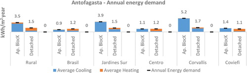
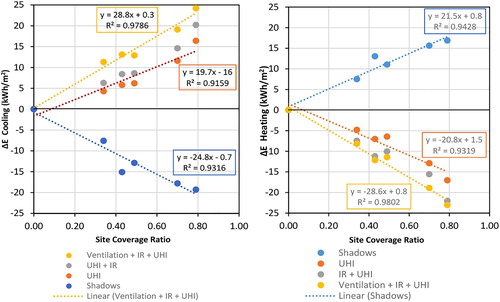
Figure 11. Correlation between the urban texture's site coverage ratio and the cooling (left) and heating (right) demand of the apartment block typology in Rome.

In Rome, the annual energy demand of urban buildings is either higher or lower than the rural one depending on the urban texture morphology (Figure 9). In Tridente and Campo Marzio, the net impact of the urban context is positive, due to the significant reduction in the heating demand determined by the UHI intensity, which balances the negative impact in summer. In all the other cases, instead, the increase in the cooling demand determined by the urban context is higher than the decrease in the heating demand, which causes a net increase in the annual demand compared to rural-open environments. Clearly, the net energy impact could change for more insulated buildings.

In Antofagasta, instead, the heating need is approximately zero and the urban heat island intensity has less impact on the annual energy demand. On the other hand, the urban shadows play a crucial role in reducing the cooling demand of urban buildings.

5. Discussion

The results of the case studies confirmed that urban climate modifies the energy performance of buildings and it should be carefully included in BPS to obtain reliable results for urban environments. In temperate climates, such as in Rome, the urban context determines significant variations in the ratio of the heating and cooling demands, causing an increase in cooling and decrease in heating compared to buildings out of the urban context. In hot-dry climates with high solar radiation, like Antofagasta, the urban context substantially modifies the building cooling demand by modifying solar gains and ventilation potential.

The overall impact of urban climate on building energy performance is thus dependent on the region's climate. More precisely, the results of the case studies showed that the solar obstructions determined by surrounding buildings have a huge impact on the building energy demand in both cities, while the other urban effects are more or less important depending on the climate of the region.

In desert climates, where solar radiation is the main cause of overheating in buildings, the urban heat island intensity in urban areas has a minor impact, comparable to that of ventilation reduction and infrared radiation exchange. In some cases, the impact of the ventilation decrease is more important than the UHI intensity in determining cooling demand changes.

In the Mediterranean climate of Rome, instead, the UHI intensity and the solar obstructions determined by surrounding buildings have comparable energy impacts, especially in the most compact and dense urban areas. The energy impacts of reduced ventilation and infrared exchange in urban areas are less important in absolute terms, but they are decisive in determining the final net energy impact of built form (if positive or negative), especially in summer.

In both cities, the highest night-time surface and air temperatures were found in the textures with higher site coverage ratios – i.e. urban compactness – such as Campo Marzio and Tridente in Rome and Coviefi and Centro in Antofagasta. On the other hand, the textures with higher building heights showed the maximum decrease of solar radiation on buildings’ facades. These two microclimate modifications have opposite impact on buildings’ energy demand. These countering effects are well explained by the correlations reported in Figure 11, showing the impact of urban shadows, air temperature increase, urban infrared radiation exchange and wind speed on the building cooling demand as a function of the ‘site coverage’ of the case studies.

Considering only urban shadows, a negative correlation (R² = 0.93) is found between the building cooling demand and the urban compactness. This means that increasing levels of compactness and urban shadows have a positive effect on the cooling energy demand in Rome. However, an opposite positive correlation (R² = 0.9159) is found between the urban compactness and the cooling demand when the UHI intensity determined by compact urban textures is considered. For this reason, these two effects tend to balance out in this climate, with a slightly higher weight of the shadows (−24.8 slope) over the UHI intensity (+19.7 slope) for the same compactness of the texture, as similarly found in previous works (Salvati, Coch, and Morganti 2017; Palme, Inostroza, and Salvati 2018). Nevertheless, when all urban climate modifications are included, the cooling demand is found to increase with the increase of urban compactness in Rome. This is because the overlapping impact of UHI intensity, infrared radiation exchange and ventilation (+28.7 slope, R² = 0.9786) in compact urban textures is higher than the beneficial effect of shadows.

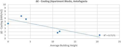
Despite similar urban microclimate modifications, no correlation was found between urban compactness and building energy demand in Antofagasta. This is explained by the different climate and energy needs in this context compared to Rome. In Antofagasta, the solar radiation is much higher than in Rome, while the daily air temperature range is smaller. For his reason, the most important variable of urban morphology turned out to be the average buildings height, which affects buildings’ solar gains and maximum urban air temperatures. A good (R² = 0.7171) negative correlation was found between the average buildings height and the cooling energy demand in the case studies analysed (Figure 12).

Figure 12. Correlation between the urban textures’ average building height and the building cooling demand variation of the apartment block typology in Antofagasta.

Finally, the two building typologies showed the same behaviour in terms of relative variation of the energy demand in urban context as opposite to rural-open environments. However, the relative energy impact is always higher in the detached house compared to the apartment block. This is due to the different shape of the two typologies and the different ratio of the external surface (envelope) to the total built volume. The detached houses have more external surface and are more affected by changes in the outdoor climate than apartment blocks.

Future developments of this research will investigate the weight of different building parameters on the energy performance in urban environments (e.g. thermal mass, insulation, percentage of glazed surfaces, operational schedules etc.).

6. Conclusion

This study described a modelling methodology to perform energy performance simulations of buildings in urban context, including all the climate modifications determined by urban built form. The methodology is applied to two building typologies in 10 urban textures of Rome and Antofagasta. A chain strategy is proposed, using existing physical and empirical methods to model the air temperature increase, solar obstructions, wind speed decrease and urban infrared environment of different urban textures and to use these outputs as boundary conditions for simulations with TRNSYS.

The case studies results confirmed that all the microclimate modifications contribute to modify the energy demand of urban buildings, but their relative impact depends on the region's climate. In Rome, the local UHI intensity and the shadows from surrounding buildings have the highest energy impact on both the cooling and the heating demand. Their relative impact increases with the increase of the urban texture compactness (or site coverage ratio). The two effects tend to balance out in terms of net energy impact on the annual demand, because buildings in the Mediterranean climate need both heating and cooling energy. However, the urban context is responsible for significant variations in the ratio of the building heating and cooling demands compared to the same building in a rural-open environment. The results also showed that in low-density urban textures, where the impact of shadows is reduced, the urban radiant environment and the reduction of wind speed determine a significant increase of the building cooling demand.

In Antofagasta, were cooling is the only energy need, the urban shadows have a higher impact than the UHI intensity on buildings’ cooling demand. Therefore, urban context may determine a significant reduction of buildings energy need, especially in urban textures with high buildings height.

The results of the case studies also showed that two morphology parameters – the site coverage ratio and the average building height – can be good predictors of the building energy performance in different urban textures. This could be applied to map the energy performance variability across a city and to foster targeted refurbishment strategies depending on the characteristics of the urban texture.

The presented simulation methodology can be applied to similar urban contexts and other building typologies and it is expected to be useful to architects, planners and modellers in understanding the relationship between urban morphology, urban microclimate and urban building energy performance, so as to improve thermal comfort and energy efficiency at the building and the urban scale.

Nomenclature

Table

Symbol	Designation	Unit
A	net opening area of windows	m^−2
A	size of the square-plan buildings in the simplified urban texture models	m
B	sum of the building size and the distance from the adjacent buildings in the simplified urban texture models	m
cd	opening discharge coefficient	-
$c_p^{+}{c}_p^{-}$	Pressure coefficients	-
H	Average building height	m
K	BS terrain roughness coefficient	-
$q_v$	Windows hourly airflow rates	m^3/h
Troad	Surface temperature of road	°C
TurbSurf	Urban Surface temperature: temperature of the opposite surface with respect to the sky used in the long wave exchange calculation in TRNSYS	°C
Twall	Surface temperature of buildings’ walls	°C
U0	canyon wind speed at ground	m s^−1
U-values	Transmittance of the component	W m^−2 K^−1
V	Wind speed at datum height	m s^−1
V(w)	wind speed at the window height	m s^−1
VFroad	View factor between the building facade and the road	-
VFw	View factor between the building facade and the surrounding facades	-
VH	Facade-to-site ratio: ratio of the building facades to the urban site area	-
VH	wind speed at the building height	m s^−1
Vm	meteorological station wind speed	m s^−1
Vurb	Urban wind speed	m s^−1
W	width of the canyon	m
Z	datum height	m
Z0	aerodynamic roughness length of the area	m
Z2	roughness length for the obstructed sub-layer	m
Α	BS terrain roughness coefficient	-
Γ	Horizontal obstruction angle of building facades	°
Δ	Vertical obstruction angle of building facades	°
Ρ	Site coverage ratio: ratio of the building footprints to the urban site area	-
$u$	along canyon-axis component of wind speed	m s^−1
$v$	cross canyon axis component of wind speed	m s^−1
$w$	Vertical component of canyon wind speed	m s^−1
$W_h$	air velocity inside the canyon at horizontal level	m s^−1
$W_t$	Total wind speed inside the canyon	m s^−1

ORCID

A. Salvati http://orcid.org/0000-0002-1449-1299

M. Palme http://orcid.org/0000-0003-1166-2926

G. Chiesa http://orcid.org/0000-0003-3783-5143

M. Kolokotroni http://orcid.org/0000-0003-4478-1868

Additional information

Funding

This work was supported by the Engineering and Physical Sciences Research Council under the project ‘Urban albedo computation in high latitude locations: An experimental approach’ (EP/P02517X/1) and by the Vice-Rectory of Research and Technological Development of UCN for one month research stay of Dr Salvati in Antofagasta.

Notes

1 Publicly available here https://github.com/Jiachen-Mao/UWG_Matlab.

2 A spreadsheet file to calculate urban wind speed based on the methodology adopted in this study is available online at the following link: https://doi.org/10.17633/rd.brunel.11371272.v1.

References

- Allard, Francis. 1998. Natural Ventilation in Buildings: A Design Handbook. London: James & James.
- Allegrini, Jonas, Viktor Dorer, and Jan Carmeliet. 2012. “Influence of the Urban Microclimate in Street Canyons on the Energy Demand for Space Cooling and Heating of Buildings.” Energy and Buildings 55 (December): 823–832. doi:10.1016/j.enbuild.2012.10.013.
- Allegrini, Jonas, Viktor Dorer, and Jan Carmeliet. 2016. “Impact of Radiation Exchange Between Buildings in Urban Street Canyons on Space Cooling Demands of Buildings.” Energy and Buildings 127: 1074–1084. doi:10.1016/j.enbuild.2016.06.073.
- British Standards Institution. 1991. “Code of Practice for Ventilation Principles and Designing for Natural Ventilation (BS 5925:1991).”
- Bueno, Bruno, Julia Hidalgo, Grégoire Pigeon, Leslie Norford, and Valery Masson. 2013. “Calculation of Air Temperatures Above the Urban Canopy Layer From Measurements at a Rural Operational Weather Station.” Journal of Applied Meteorology and Climatology 52 (2): 472–483. doi:10.1175/JAMC-D-12-083.1.
- Bueno, Bruno, Leslie Norford, Julia Hidalgo, and Grégoire Pigeon. 2013. “The Urban Weather Generator.” Journal of Building Performance Simulation 6 (4): 269–281. doi:10.1080/19401493.2012.718797.
- Bueno, Bruno, Leslie Norford, Grégoire Pigeon, and Rex Britter. 2011. “Combining a Detailed Building Energy Model with a Physically-Based Urban Canopy Model.” Boundary-Layer Meteorology 140 (3): 471–489. doi:10.1007/s10546-011-9620-6.
- Burdett, Ricky, and Deyan Sudjic. 2007. The Endless City: The Urban Age Project by the London School of Economics and Deutsche Bank’s Alfred Herrhausen Society. London: Phaidon Press.
- Caton, P. G. F. 1977. “Standardised Maps of Hourly Mean Wind Speed Over the United Kingdom and Some Implications Regarding Wind Speed Profiles.” In Proceedings of the Fourth International Conference on Wind Effects on Buildings and Structures. Heathrow 1975, edited by Keith J. Eaton, 7–21. London: Cambridge University Press.
- Chan, A. L. S. 2011. “Developing a Modi Fi Ed Typical Meteorological Year Weather Fi Le for Hong Kong Taking Into Account the Urban Heat Island Effect.” Building and Environment 46 (12): 2434–2441. doi:10.1016/j.buildenv.2011.04.038.
- Chatzipoulka, Christina, Raphaël Compagnon, and Marialena Nikolopoulou. 2016. “Urban Geometry and Solar Availability on Façades and Ground of Real Urban Forms: Using London as a Case Study.” Solar Energy 138: 53–66. doi:10.1016/j.solener.2016.09.005.
- Chatzipoulka, Christina, and Marialena Nikolopoulou. 2018. “Urban Geometry, SVF and Insolation of Open Spaces: London and Paris.” Building Research and Information 46 (8): 881–898. doi:10.1080/09613218.2018.1463015.
- Chatzipoulka, Christina, Marialena Nikolopoulou, and Richard Watkins. 2015. “The Impact of Urban Geometry on the Radiant Environment in Outdoor Spaces.” ICUC9 - 9th International Conference on Urban Climate Jointly with 12th Symposium on the Urban Environment The. Toulouse, France.
- Chiesa, Giacomo, and Mario Grosso. 2017a. “Cooling Potential of Natural Ventilation in Representative Climates of Central and Southern Europe of Central and Southern Europe.” International Journal of Ventilation 16 (2): 84–98. doi:10.1080/14733315.2016.1214394.
- Chiesa, Giacomo, and Mario Grosso. 2017b. “Environmental and Technological Design: A Didactical Experience towards a Sustainable Design Approach.” Proceedings of the XV International Forum Le Vie Dei Mercanti, World Heritage and Disaster, edited by Gambardella C., 944–53. Naples 15-Capri 16-17 June: La scuola di Pitagora.
- Costola, Daniel, Bert Blocken, and J. L. M. Hensen. 2009. “Overview of Pressure Coefficient Data in Building Energy Simulation and Airflow Network Programs.” Building and Environment 44 (10): 2027–2036. doi:10.1016/j.buildenv.2009.02.006.
- Crawley, Drury B. 2008. “Estimating the Impacts of Climate Change and Urbanization on Building Performance.” Journal of Building Performance Simulation 1 (2): 91–115. doi:10.1080/19401490802182079.
- Di Bernardino, Annalisa, Paolo Monti, Giovanni Leuzzi, and Giorgio Querzoli. 2015. “Water-Channel Study of Flow and Turbulence Past a Two-Dimensional Array of Obstacles.” Boundary-Layer Meteorology 155 (1): 73–85. doi:10.1007/s10546-014-9987-2.
- Frayssinet, Loïc, Lucie Merlier, Frédéric Kuznik, Jean Luc Hubert, Maya Milliez, and Jean Jacques Roux. 2018. “Modeling the Heating and Cooling Energy Demand of Urban Buildings at City Scale.” Renewable and Sustainable Energy Reviews 81: 2318–2327. doi:10.1016/j.rser.2017.06.040.
- Futcher, Julie, Tristan Kershaw, and Gerald Mills. 2013. “Urban Form and Function as Building Performance Parameters.” Building and Environment 62: 112–123. doi:10.1016/j.buildenv.2013.01.021.
- Futcher, Julie, Gerald Mills, and Rohinton Emmanuel. 2018. “Interdependent Energy Relationships Between Buildings at the Street Scale.” Building Research & Information 46 (8): 829–844. doi:10.1080/09613218.2018.1499995.
- Georgakis, Chrissa, and Mattheos Santamouris. 2006. “Experimental Investigation of Air Flow and Temperature Distribution in Deep Urban Canyons for Natural Ventilation Purposes.” Energy and Buildings 38 (4): 367–376. doi:10.1016/j.enbuild.2005.07.009.
- Georgakis, Chrissa, and Mattheos Santamouris. 2008. “On the Estimation of Wind Speed in Urban Canyons for Ventilation Purposes-Part 1: Coupling Between the Undisturbed Wind Speed and the Canyon Wind.” Building and Environment 43 (8): 1404–1410. doi:10.1016/j.buildenv.2007.01.041.
- Ghiaus, Christian, Francis Allard, C. Georgiakis, Mat Santamouris, Claude-Alain Roulet, M. Germano, F. Tillenkamp, et al. 2004. “URBVENT WP1 Final Report: Soft Computing of Natural Ventilation Potential.” URBVENT: Natural Ventilation in Urban Areas - Potential Assessment and Optimal Façade Design. European Commision. doi:10.4324/9781849772068.
- Giridharan, Renganathan, and Rohinton Emmanuel. 2018. “The Impact of Urban Compactness, Comfort Strategies and Energy Consumption on Tropical Urban Heat Island Intensity: A Review.” Sustainable Cities and Society 40 (October 2017): 677–687. doi:10.1016/j.scs.2018.01.024.
- Grosso, Mario. 1992. “Wind Pressure Distribution Around Buildings: A Parametrical Model.” Energy & Buildings 18: 101–131. doi: 10.1016/0378-7788(92)90041-E
- Grosso, Mario. 2017. Il Raffrescamento Passivo Degli Edifici in Zone a Clima Temperato (Passive Cooling of Buildings in Temperate Climate Zones). IV. Sant’Arcangelo di Romagna: Maggioli.
- Holzer, Peter, and Theofanis Psomas. 2018. Ventilative Cooling Source Book - IEA EBC ANNEX 62. Aalborg: Aalborg University.
- Hotchkiss, R. S., and F. H. Harlow. 1973. “Air Pollution Transport in Street Canyons.” Repot for: Office of research and monitoring U.S. Environmental protection Agency.
- Ignatius, Marcel, Nyuk Hien Wong, and Steve Kardinal Jusuf. 2016. “The Significance of Using Local Predicted Temperature for Cooling Load Simulation in the Tropics.” Energy and Buildings 118: 57–69. doi:10.1016/j.enbuild.2016.02.043.
- Isaac, Morna, and Detlef P. van Vuuren. 2009. “Modeling Global Residential Sector Energy Demand for Heating and Air Conditioning in the Context of Climate Change.” Energy Policy 37: 507–521. doi:10.1016/j.enpol.2008.09.051.
- Kavgic, M., A. Mavrogianni, D. Mumovic, A. Summerfield, Z. Stevanovic, and M. Djurovic-Petrovic. 2010. “A Review of Bottom-up Building Stock Models for Energy Consumption in the Residential Sector.” Building and Environment 45 (7): 1683–1697. doi:10.1016/j.buildenv.2010.01.021.
- Khoshdel, Saber, Mohammad Heidarinejad, Jiying Liu, and Jelena Srebric. 2017. “Quantifying the Impact of Urban Wind Sheltering on the Building Energy Consumption.” Applied Thermal Engineering 116: 850–865. doi:10.1016/j.applthermaleng.2017.01.044.
- Knoll, B., J. C. Phaff, and W. F. de Gids. 1995. “Pressure Simulation Program.” Iplementing the Results of Ventilation Research. 16th AIVC Conference, 233–41. Palm Springs, USA.
- Kolokotroni, Maria, I. Giannitsaris, and Ricard Watkins. 2006. “The Effect of the London Urban Heat Island on Building Summer Cooling Demand and Night Ventilation Strategies.” Solar Energy 80 (4): 383–392. doi:10.1016/j.solener.2005.03.010.
- Kolokotroni, Maria, and Renganathan Giridharan. 2008. “Urban Heat Island Intensity in London: An Investigation of the Impact of Physical Characteristics on Changes in Outdoor Air Temperature During Summer.” Solar Energy 82: 986–998. doi:10.1016/j.solener.2008.05.004.
- Kolokotroni, Maria, X. Ren, Michael Davies, and Anna Mavrogianni. 2012. “London’s Urban Heat Island: Impact on Current and Future Energy Consumption in Office Buildings.” Energy and Buildings 47 (April): 302–311. doi:10.1016/j.enbuild.2011.12.019.
- Lauzet, Nicolas, Benjamin Morille, Thomas Leduc, and Marjorie Musy. 2017. “What Is the Required Level of Details to Represent the Impact of the Built Environment on Energy Demand?” Procedia Environmental Sciences 38: 611–618. doi:10.1016/j.proenv.2017.03.140.
- Lauzet, Nicolas, Auline Rodler, Marjorie Musy, Marie-hélène Azam, Sihem Guernouti, Dasaraden Mauree, and Thibaut Colinart. 2019. “How Building Energy Models Take the Local Climate Into Account in an Urban Context – A Review.” Renewable and Sustainable Energy Reviews 116 (August): 109390. doi:10.1016/j.rser.2019.109390.
- Li, Xiaoma, Yuyu Zhou, Sha Yu, Gensuo Jia, Huidong Li, and Wenliang Li. 2019. “Urban Heat Island Impacts on Building Energy Consumption: A Review of Approaches and Fi Ndings.” Energy 174: 407–419. doi:10.1016/j.energy.2019.02.183.
- Lundgren, Karin, and Tord Kjellstrom. 2013. “Sustainability Challenges From Climate Change and Air Conditioning Use in Urban Areas.” Sustainability 3116–3128. doi:10.3390/su5073116.
- Mao, Jiachen, Yangyang Fu, Afshin Afshari, Peter R. Armstrong, and Leslie K. Norford. 2018. “Optimization-Aided Calibration of an Urban Microclimate Model Under Uncertainty.” Building and Environment 143 (July): 390–403. doi:10.1016/j.buildenv.2018.07.034.
- Mao, Jiachen, Joseph H. Yang, Afshin Afshari, and Leslie K. Norford. 2017. “Global Sensitivity Analysis of an Urban Microclimate System Under Uncertainty: Design and Case Study.” Building and Environment 124: 153–170. doi:10.1016/j.buildenv.2017.08.011.
- Masson, Valéry. 2000. “A Physically-Based Scheme for the Urban Energy Budget in Atmospheric Models.” Boundary-Layer Meteorology 94: 357–397. doi: 10.1023/A:1002463829265
- Nakamura, Y., and T. R. Oke. 1988. “Wind, Temperature and Stability Conditions in an East-West Oriented Urban Canyon.” Atmospheric Environment (1967) 22 (12): 2691–2700. doi:10.1016/0004-6981(88)90437-4.
- Nakano, Aiko, Bruno Bueno, Leslie Norford, and Christoph F Reinhart. 2015. “Urban Weather Generator User Interface Development: New Workflow for Integrating Urban Heat Island Effect in Urban Design Process.” ICUC9 - 9th International Conference on Urban Climate Jointly with 12th Symposium on the Urban Environment 1 (2014). doi:10.1016/S1091853104001594.
- Nardecchia, Fabio, Annalisa di Bernardino, Francesca Pagliaro, Paolo Monti, Giovanni Leuzzi, and Luca Gugliermetti. 2018. “CFD Analysis of Urban Canopy Flows Employing the V2F Model: Impact of Different Aspect Ratios and Relative Heights.” Advances in Meteorology 2018: Article ID 2189234. doi: 10.1155/2018/2189234
- Nicholson, Sharon E. 1975. “A Pollution Model for Street-Level Air.” Atmospheric Environment (1967) 9 (1): 19–31. doi:10.1016/0004-6981(75)90051-7.
- Oke, T. R. 1988. “Street Design and Urban Canopy Layer Climate.” Energy and Buildings 11: 103–113. doi:10.1016/0378-7788(88)90026-6.
- Oke, T. R., G. Mills, A. Christen, and J. A. Voogt. 2017. Urban Climates. Cambridge: Cambridge University Press. doi:10.1017/9781139016476.
- Palme, Massimo, Claudio Carrasco, and Andrea Lobato. 2016. “Quantitative Analysis of Factors Contributing to Urban Heat Island Effect in Cities of Latin-American Pacific Coast.” Procedia Engineering 169: 199–206. doi:10.1016/j.proeng.2016.10.024.
- Palme, Massimo, Luis Inostroza, and Agnese Salvati. 2018. “Technomass and Cooling Demand in South America: A Superlinear Relationship?” Building Research & Information 46 (Issue 8: Urban form, density & microclimate): 864–880. doi:10.1080/09613218.2018.1483868.
- Palme, Massimo, and Agnese Salvati. 2018. “UWG -TRNSYS Simulation Coupling for Urban Building Energy Modelling.” Proceedings of BSO 2018: 4th Building Simulation and Optimization Conference, Cambridge, UK: 11-12 September 2018, 635–41. http://www.ibpsa.org/proceedings/BSO2018/6B-4.pdf.
- Ramponi, Rubina, Adriana Angelotti, and Bert Blocken. 2014. “Energy Saving Potential of Night Ventilation: Sensitivity to Pressure Coefficients for Different European Climates.” Applied Energy 123: 185–195. doi:10.1016/j.apenergy.2014.02.041.
- Ratti, Carlo, Nick Baker, and Koen Steemers. 2005. “Energy Consumption and Urban Texture.” Energy and Buildings 37 (7): 762–776. doi:10.1016/j.enbuild.2004.10.010.
- Reinhart, Christoph F., and Carlos Cerezo Davila. 2016. “Urban Building Energy Modeling - A Review of a Nascent Field.” Building and Environment. doi:10.1016/j.buildenv.2015.12.001.
- Salvati, Agnese, Helena Coch, and Carlo Cecere. 2015. “Urban Morphology and Energy Performance: The Direct and Indirect Contribution in Mediterranean Climate.” In PLEA2015 Architecture in (R)Evolution - 31st International PLEA Conference, edited by Mario Cucinella, Giulia Pentella, Alba Fagnani, and Luca D’Ambrosio. Bologna, Italy.
- Salvati, Agnese, Helena Coch, and Carlo Cecere. 2016. “Urban Heat Island Prediction in the Mediterranean Context: An Evaluation of the Urban Weather Generator Model.” ACE: Architecture, City and Environment = Arquitectura, Ciudad y Entorno 11 (32): 135–156. doi:10.5821/ace.11.32.4836.
- Salvati, Agnese, Helena Coch, and Carlo Cecere. 2017. “Assessing the Urban Heat Island and Its Energy Impact on Residential Buildings in Mediterranean Climate: Barcelona Case Study.” Energy and Buildings 146: 38–54. doi:10.1016/j.enbuild.2017.04.025.
- Salvati, Agnese, Helena Coch, and Michele Morganti. 2017. “Effects of Urban Compactness on the Building Energy Performance in Mediterranean Climate.” Energy Procedia 499–504. doi:10.1016/j.egypro.2017.07.303.
- Salvati, Agnese, Paolo Monti, Helena Coch, and Carlo Cecere. 2019. “Climatic Performance of Urban Textures: Analysis Tools for a Mediterranean Urban Context.” Energy and Buildings 185: 162–179. doi:10.1016/j.enbuild.2018.12.024.
- Salvati, Agnese, Massimo Palme, and Luis Inostroza. 2017. “Key Parameters for Urban Heat Island Assessment in A Mediterranean Context: A Sensitivity Analysis Using the Urban Weather Generator Model.” IOP Conference Series: Materials Science and Engineering 245: 082055. doi:10.1088/1757-899X/245/8/082055.
- Santamouris, Mattheos, Chrissa Georgakis, and A. Niachou. 2008. “On the Estimation of Wind Speed in Urban Canyons for Ventilation Purposes-Part 2: Using of Data Driven Techniques to Calculate the More Probable Wind Speed in Urban Canyons for Low Ambient Wind Speeds.” Building and Environment 43 (8): 1411–1418. doi:10.1016/j.buildenv.2007.01.042.
- Steemers, Koen, Nick Baker, David Crowther, Jo Dubiel, and Marialena Nikolopoulou. 1998. “Radiation Absorption and Urban Texture.” Building Research & Information 26 (2): 103–112. doi:10.1080/096132198370029.
- Stewart, I. D., and T. R. Oke. 2012. “Local Climate Zone for Urban Temperature Studies.” Bulletin of the American Meteorological Society 93 (12): 1879–1900. doi: 10.1175/BAMS-D-11-00019.1
- Swami, M. V., and S. Chandra. 1987. Procedures of Calculating Natural Ventilation Airflow Rates in Buildings. Final Report FSEC-CR-163-86. ASHRAE Research Project 448-RP. Cape Canaveral: Florida Solar Energy Center.
- Vallati, A., L. Mauri, C. Colucci, and P. Ocłoń. 2017. “Effects of Radiative Exchange in an Urban Canyon on Building Surfaces’ Loads and Temperatures.” Energy and Buildings 149: 260–271. doi:10.1016/j.enbuild.2017.05.072.
- Watkins, Richard, J. Palmer, Maria Kolokotroni, and P. Littlefair. 2002. “The Balance of the Annual Heating and Cooling Demand Within the London Urban Heat Island.” Building Services Engineering Research and Technology 23 (4): 207–213. doi: 10.1191/0143624402bt043oa
- Yamartino, Robert J., and Götz Wiegand. 1986. “Development and Evaluation of Simple Models for the Flow, Turbulence and Pollutant Concentration Fields Within an Urban Street Canyon.” Atmospheric Environment (1967) 20 (11): 2137–2156. doi:10.1016/0004-6981(86)90307-0.
- Yang, Xiaoshan, Lihua Zhao, Michael Bruse, and Qinglin Meng. 2012. “An Integrated Simulation Method for Building Energy Performance Assessment in Urban Environments.” Energy and Buildings 54 (November): 243–251. doi:10.1016/j.enbuild.2012.07.042.
- Zinzi, Michele, and Emiliano Carnielo. 2017. “Impact of Urban Temperatures on Energy Performance and Thermal Comfort in Residential Buildings. The Case of Rome, Italy.” Energy & Buildings. doi:10.1016/j.enbuild.2017.05.021.
- Zinzi, Michele, Emiliano Carnielo, and Benedetta Mattoni. 2018. “On the Relation Between Urban Climate and Energy Performance of Buildings. A Three-Years Experience in Rome, Italy.” Applied Energy 221 (March): 148–160. doi:10.1016/j.apenergy.2018.03.192.