The first world championship in cybernetic building optimization

ABSTRACT

The World Championship in Cybernetic Building Optimization (WCCBO) was held in 2019 to test participants’ ability to optimize buildings cybernetically. Office buildings with a total floor area of 10,000 m² were built in cyberspace, one for each of the 33 participating teams. The cyber buildings were controlled by BACnet, and the participants competed to show their operational skills by tuning the HVAC system of their respective cyber buildings online. The ability of optimization was evaluated in terms of both energy consumption and thermal comfort, and their scores were published online in real-time. A total of 339 different operations were tested during the two-month competition period. The top-ranked team succeeded in reducing energy consumption and thermally dissatisfied occupant rate by 12.1% and 21.0%, respectively. In this paper, we report on the examination of the rules and schedule of this championship as well as the analysis of the participants’ scores.

KEYWORDS:

• Emulator
• HVAC
• operation
• simulation
• optimization
• BACnet

1. Introduction

Energy consumption related to buildings accounts for approximately 40% of total energy consumption worldwide (IEA 2008).

The life cycle energy of a building can be divided into construction and operational phases, most of which occurs during the operational phase. In recent years, the number of cases of buildings whose energy performance has been improved by a large initial investment has been increasing, and the ratio of energy consumption at the construction stage tends to also increase (Mohammed et al. 2013). However, according to the review by Sartori and Hestnes (2007) and the study of Chau, Leung, and Ng (2015), comparing the life-cycle energy consumption between traditional and energy-saving buildings, more than 50% of life-cycle energy is spent in the operational phase, even with energy-saving buildings. Therefore, the problem of how to control and operate the buildings’ HVAC (Heating, ventilation, and air conditioning) system should be sufficiently considered, even today.

Commonly, computer simulations are used to predict the energy consumption of a building during the operation phase. This is because a building is a complex system, having a large number of elements with non-linear behavior, and its energy consumption is, therefore, difficult to predict by hand calculation.

General building energy simulation software predicts the energy consumption for specific conditions, and the settings of these conditions can be changed. These are, for example, (1) wall and insulation materials and thickness, machine efficiency, (2) control parameters, or (3) outside air conditions. The first condition are hardware specifications that can be changed during the design and construction phase, the second condition can be changed during the operational phase, and the third condition cannot be changed by humans.

By solving this inverse problem, it is possible to estimate conditions (hardware specifications and control parameters) that minimize the energy consumption in the operational phase. The inverse problem is the problem of estimating the causal factors x_i such that the observed value y becomes a desired value with respect to the model represented by y = f [x_i (i = 1, 2, … n)] (Zhang et al. 2015; Rouchier 2018). In the building energy simulation, y is the energy consumption, and x_i are hardware specifications and control parameters.

However, for the energy minimization applied by the inverse problem to be effective, the simulation model must accurately predict the energy consumption of a real building. In fact, it has been pointed out that the two do not always match, and this gap is called ‘Performance Gap’ (Wilde 2014).

Specific causes of such a gap include, for example, the following: (1) The model does not completely formulate everything in accordance with reality and is limited by some abstraction. (2) Since the connection of components and the setting of parameters are usually performed by humans, the results differ depending on their skill. Improper input produces meaningless results, called the ‘Garbage In Garbage Out’ rule. (3) Real buildings are used on a different schedule than assumed by the simulation. (4) In a real building, the ideal control assumed by the simulation model is not realized (Khoury, Alameddine, and Hollmuller 2017). These are issues of the ‘Limitations of energy modeling’, some of which are discussed in detail at CIBSE (2015). To eliminate the Performance Gap, these issues must be resolved.

The aim of this study is to eliminate the gap caused by the assumption of an ideal control (cf. point 4.). The reason for providing the assumption of an ideal control is that modeling all control mechanisms requires a lot of time and effort to set the parameters of the model, and significantly increases the calculation time. On the other hand, in a real building, such ideal control cannot be automatically realized, so that a difference occurs between the calculation result and reality. Two specific examples are shown below.

The first example is the time delay of the heat source model. Most heat source models used in building energy simulations are static models, and it is assumed that if chilled/hot water is required, it can be supplied instantaneously. When such a model is used, unlike in the case of an actual building, it is not necessary to estimate the start-up time required for the heat source to supply water at a set temperature point and to consider an appropriate starting time. In some real buildings, to avoid the risk of the inability to cool or heat, the heat source may be started up much sooner than needed, consuming more energy than estimated in the simulation.

Another example is the calculation of water and air flow. Many models do not use a circuit network model, and it is assumed that the water and air flow can be adjusted to exactly the values required by each device. Therefore, whether the control of the valve or the damper is good or bad is not represented in the model. These control failures not only affect the energy consumption of the pump or fan but also increase the energy consumption by an oversupply of heat or worsen the thermal environment by an insufficient supply of heat.

There are two approaches to reduce the gap described above. One approach is to tune the equipment sufficiently to eliminate control failures in the actual building and bring it closer to the ideal state. Another approach is to express the control failure with a simulation model.

To date, however, has not been possible to quantify the engineer's ability to tune, so either of these two approaches are difficult to employ. To adopt the first approach, it is necessary to educate a large number of engineers with high tuning skills. However, if the engineer’s ability cannot be quantified, the level of education cannot be determined. To adopt the second approach, it is necessary to formulate the risk of control failures due to the engineer’s poor ability. However, this risk cannot be expressed unless the variation in the abilities of engineers can be observed quantitatively.

The reason that it is difficult to quantitatively evaluate the tuning ability is that a building is a one-piece product and tends to be very heterogeneous. Since different hardware has varying energy consumption, simply comparing the difference in energy consumption of different buildings does not reveal the difference in the ability of the engineer who tuned the control.

For a pure comparison of tuning abilities, the various conditions affecting the energy consumption of a building should be exactly the same, but in reality, such uniform conditions cannot be met.

When the comparison in a real building is not an option, an alternative is to use a simulation model. With a simulation model, buildings under exactly the same conditions can be easily copied innumerably. Of course, the simulation model used here does not assume the ideal controls that cause a gap as described above. According to the above example, the heat capacity and the time delay of the heat source are mathematically expressed, the network of pipes and ducts is solved, and control parameters for these are made operable by a user.

A highly realistic simulation model that can be used for such a purpose is generally called an emulator. The use of emulators in the building equipment field began with a study reported in Annex 17 of the International Energy Agency (IEA) in the 1990s (Lebrun and Wang 1993; Vaezi-Nejad et al. 1991; IEA 1997). Later, IEA Annex 25 examined applications for fault detection (IEA 1999) and, more recently, Bushby et al. (2001, 2010) developed a comprehensive emulator that combines air conditioning and fire simulations (Virtual Cybernetic Building Testbed: VCBT). The authors also developed an emulator system for evaluating the tuning ability of equipment, which can predict not only the energy consumption, but also the thermal sensing of office workers (Togashi and Miyata 2019).

We held a championship to compete for the purpose of quantitatively evaluating the tuning ability by using this emulator system. Promoting the development of new tuning technologies, improving the tuning skills of the participants, and quantitatively capturing the variation in building performance caused by the tuning ability, were also the purpose of the competition. In this report, we outline the rules, schedule, attributes of the participants, and results of this championship.

2. References for our competition

In the past, several attempts have been made to promote technological developments in the field of building equipment through competition. These precedents served as a reference for designing our championship.

2.1 The Great energy Predictor Shootout

The best-known competition in this field is the energy prediction competition conducted by the American Society of Heating, Refrigerating and Air-Conditioning Engineers (ASHRAE; Technical Committee 4.7 and 1.5) in the 1990s. The details of this competition are reported by Kreider and and Haberl (1994).

At the time, various new methods such as the neural network back propagation algorithm (Rumelhart, Hinton, and Williams 1986) were being developed to solve the prediction problems of nonlinear systems with time delays. In this context, the Great Energy Predictor Shootout I was carried out to competitively compare prediction methods and introduce knowledge from other related fields to that of building management.

The competition used six months of building operation data collected at a university facility in Texas (with a total floor area of approximately 30,000 m²). Detailed information on the building was not disclosed to the participants until the end of the competition. The six-month data were divided into a four-month interval (September to the end of December, 1989) and a two-month interval (January to the end of February, 1990), which were used, respectively, as training data for constructing a prediction model and test data for evaluating the prediction performance for unknown inputs. The data items to be predicted (hereafter, ‘output data’) were building power consumption and chilled and heating water load, while the data items that could be used for the prediction (hereafter, ‘input data’) were the outdoor air conditions (dry bulb temperature, absolute humidity, wind speed, and horizontal solar radiation). Training data were provided as sets of input and output data, while only input data were provided as test data.

A total of 150 teams obtained training data for competing in the participation. Of these, 21 teams continued in the competition till the end. Test data covering the period of January 1st to February 28th, 1990 were provided sequentially. The training data included data from Christmas and the New Year holidays, during which the energy consumption was lower than usual. Abnormal data caused by pipe-freezing were included in data for the extremely cold season. The sources of this information were not conveyed to the participants, who had to independently determine how to handle abnormal data.

The performance of the prediction model was evaluated using the coefficient of variation (CV) shown in Equation (1), in which y_data,i, y_pred,i, y_data, and n are, respectively, the data value of the dependent variable corresponding to a particular set of independent variable values, the predicted dependent variable value for the same set of independent variables, the mean value of the dependent variable testing data set, and the number of data records in the testing set. (1) $CV=\frac{\sqrt{{\sum }_{i=1}^n{\left(y_{pred,i}-y_{data,i}\right)}^2}}{n\cdot {\overline{y}}_{data}}$(1) In addition to an overall report on the competition by Kreider and and Haberl (1994), many of the participants individually reported their own prediction methods (Feuston and Thurtell 1994; Iijima et al. 1994; Kawashima 1994; MacKay 1994; Ohlsson et al. 1994; Stevenson 1994).

2.2 The Great energy Predictor Shootout II

Following the success of The Great Energy Predictor Shootout, a second competition was held in 1994 (Haberl and Thamilseran 1996). In addition to the university facilities that were targeted during the first round of the competition, university facilities with a total floor area of approximately 14,000 m² were added to the prediction target. The training data were placed on an FTP server, making it possible for any individual to obtain the data necessary for participation. Despite this, there were fewer participants than in the first round: only 50 individuals accessed the ‘readme.txt’ on the FTP server describing the details of the competition; 11 individuals downloaded the data used in the competition and only 4 teams participated in and completed the competition. An additional goal of this second competition was to evaluate the energy savings of a retrofitted building. The participants were first given training and test data for both buildings prior to the energy saving improvement, and they competed in predicting the modeled energy performance in the same manner as in the first contest. They were then provided operational data obtained after the retrofit and tasked with modeling the effects of the retrofit based on the difference between the pre- and post-energy consumption. The effect of the retrofit was then estimated from the difference between this value and the actual measured one.

As in the first round, each participant individually reported on the prediction methods they used in the second round of the competition (Chonan, Nishida, and Matsumoto 1996; Jang, Bartlett, and Nelson 1996; Katipamula 1996; Dodier and Henze 1996).

2.3 Heat load prediction Public competition

The Heat Load Prediction Public Competition was conducted as part of the activities of the Thermal Storage Optimization Committee organized by the Society of Heating, Air-Conditioning and Sanitary Engineers of Japan (SHASE) during 1995–1998 (SHASE 1998). To optimize the heat source operation of a heat storage-type air conditioning system, it is necessary to predict the next-day heat load. To assess the various heat load prediction methods that had been proposed at the time, the committee held a public benchmark competition to compare the methods.

Two competitions – denoted as trials I and II, respectively in this paper – were held in August and October of 1998. The goal of both trials was to predict the next-day heat load. During trial I, the next-day weather conditions, indoor temperature and humidity conditions, and HVAC operation schedule – none of which can be obtained precisely in advance in reality – were provided. For trial II, a more realistic case was applied in which only the weather forecast and HVAC operational schedule were provided.

Eighteen and 14 teams, respectively, participated in trials I and II. During trial I, e-mails were used to exchange information such as prediction results, with the organizer’s side sending day-ahead input data for prediction to the participating teams via e-mail, and the participants making predictions based on this information and sending the prediction results back to the organizer’s side. After confirming the reply, the organizer would send the next day’s input data.

This approach was quite complicated and, in particular, it was impossible to prevent rule violations in terms of information collaboration among participants. Therefore, in trial II, a system in which all input and output data were provided from the beginning was instituted under an assumption of participant conscientiousness. For both trials I and II, the performance of the predictive models was evaluated in terms of the sum of the squared difference (SSD) between the predicted and actual results, as shown in Equation (2).

Many participants reported on the heat load prediction methods they used in this championship. The championship winner was a researcher in the field of information engineering who did not specialize in building equipment, suggesting that the championship succeeded in introducing expertise from different fields. (2) $SSD=\sum _{i=1}^n(y_{pred,i}-y_{data,i}{)}^2$(2)

2.4 Championship policies based on precedents

The competitions described above took place during the 1990s, and although some involved the use of FTP servers and email, much of the work was performed manually. In the heat load prediction competition of SHASE, the workload involved in exchanging e-mails with the participants was heavy, and therefore, the system used to evaluate the results was changed for trial II. To increase the number of participants and expand the scale of the competition, it was necessary to establish a system that automates clerical work as much as possible. In particular, automation was essential for our championship because, unlike the preceding competitions, the evaluated scores had to be obtained via simulation in addition to simple comparisons with the correct answer in terms of the energy consumption or heat load.

Many of the participants of the previous competitions reported their calculation methods. Future development of this field will benefit from the knowledge of not only which approaches win and lose, but also what kind of performance is obtained using a specific type of method. Despite the desirability of having participants disclose the methods they use in competition, the decision to disclose this information rests solely with them; the organizers cannot force disclosures. Accordingly, we decided to save and make public the operational data for the highest-graded approaches. It was possible to obtain an overview of individual participant approaches by analyzing these data.

In general, operational data often include abnormal values reflecting measurement problems or instances with broken or malfunctioning equipment. Additionally, even in cases in which the equipment is operating normally, the measured values can gradually shift as a result of aging. For example, the data distributed to the participants of the Great Energy Predictor Shootout I included abnormal values arising from extended holidays and a broken pipe. The method to be used to deal with such abnormal values depends on operational ability. We therefore initially considered testing resilience by intentionally including an abnormal value, but eventually decided not to because the task became too difficult to implement during our championship. In the future, however, this approach should be considered to increase the difficulty of the competition.

One reason for the decreased number of participants during the second Great Energy Predictor Shootout is that the theme was changed to the prediction of energy-saving renovation effects. Although this is a valuable theme, it cannot clearly differentiate between winners and losers. To increase the number of participants, it is necessary to clarify the conditions for victory and defeat and to gamify the competition (i.e. impart a higher ‘fun component’ to it). Therefore, in our championship, the method for calculating the score was clearly demonstrated prior to the event, and the participants’ scores were displayed in real time during the competition period.

It should be noted that our championship was more complicated than previous events, as the purpose of our competition was not to predict a single number such as heat load or energy consumption, but to tune thousands of parametric controls for improving energy and comfort. The participants from the information technology field were generally not expected to understand the details of the building equipment physical system, while the participants from the building operation and management field were generally expected to have no experience with programs for communicating with BACnet. For this reason, a simple ‘readme’ file was insufficient for providing the information needed for participation; instead, a detailed manual that described how to implement BACnet communication programs and tutorials on building optimization were developed.

Table 1 shows a comparison of previous similar competitions and this championship.

Table 1. Comparison of previous similar competitions and this championship.

	The great energy predictor shootout		Heat load prediction public competition
Name	I	II	First trial	Second trial	This championship (WCCBO)
Competition period	1/1/1990–2/28/1990	6/1/1994–11/1/1994	8/1/1998–8/31/1998	10/1998	6/7/2019–8/7/2019
Target of the competition	Predicting the next day’s energy consumption	Predicting the next day’s energy consumption	Predicting the next day’s heat load	Predicting the next day’s heat load	Optimizing energy use and thermal comfort
Target building (Total floor area)	Real university building (30,000 m^2)	Real university building (14,000 m^2)	Real research center building (38,400 m^2)	Real office building (5400 m^2)	Virtual office building (10,000 m^2)
Evaluation criteria	Coefficient of variation (Equation 1)	Coefficient of variation (Equation 1)	Sum of the squared difference (Equation 2)	Sum of the squared difference (Equation 2)	Effective energy reduction ratio (described in Section 3.1)
Number of participants	21	4	17	13	34 (described in Section 3.3)
Data submission method	Submit to organizer in bulk	Submit to organizer in bulk	Submit to organizer by email every day	Submit to organizer in bulk	Submit to server at any time
Publication of score	After the competition	After the competition	After the competition	After the competition	Calculated immediately on the server (in real time)

3. Preparations for the world championship of Cybernetic building optimization

In this section, we explain the rules of our championship (evaluation method and schedule) and provide information on the participants.

3.1 Determination of evaluation criteria

As already mentioned, the championship was hosted on the emulator system described in our previous report (Togashi and Miyata 2019). This system can evaluate how energy performance and thermal comfort change with respect to the default operational parameters using the energy reduction ratio (ERR) and the dissatisfied reduction ration (DRR) given in Equations (3) and (4), respectively, in which E is the primary energy consumption, D is the dissatisfaction rate, the subscript r indicates default operation, and the subscript opt indicates optimized operation. (3) $\begin{array}{rl}ERR& =\frac{E_r-E_{opt}}{E_r},\end{array}$(3) (4) $\begin{array}{rl}DRR& =\frac{D_r-D_{opt}}{D_r}.\end{array}$(4) The thermal load calculation model and the static equipment models used in the emulator were verified using the BESTEST (Togashi and Tanabe 2009) and SHASE guidelines (Ono, Ito, and Yoshida 2017; SHASE 2016), respectively. For details on each component in the emulator system, such as calculating the physical model for each equipment model or occupant thermal sensation, please refer to our previous report.

To determine the winner, the energy-savings and thermal-comfort indicators were integrated into a single score. Searching for an optimal point in which several performance indexes are combined in this manner is called multi-objective optimization. According to Nguyen, Reiter, and Rigo (2014), approximately 40% of the optimization research in the building equipment field involves solving multi-objective optimization problems. The simplest approach to combine multiple indicators is a linear combination, as represented by Equation (5), in which w_ERR is a weighting factor that takes a value ranging from 0 to 1. (5) $w_{ERR}ERR+\left(1-w_{ERR}\right)DRR$(5)

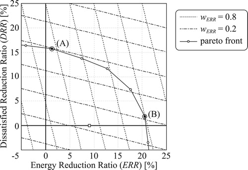
If the weighting factor value in Equation (5) is biased, a problem may occur, as described later. Figure 1 is an example of pareto optimum solution selected by a linear combination function. Contour lines of two linear combination functions with different weighting factors are drawn. A one-dot chain line has a small weighting factor, and a dotted line has a large weighting factor. The solid curve is a pareto front that can be realized by changing the operation. There is a trade-off relationship between reduction in energy consumption and the dissatisfaction rate. Therefore, we note a downward trend. In addition, the amount of dissatisfaction that can be reduced by using one unit of additional energy will degressively decrease, resulting in a convex shape in the area to the upper right. For linear combination functions with a small weighting factor, the optimal solution is (A), whereas the optimal solution for large weighting factors is (B). As is apparent from the figure, changing the weighting factor significantly modifies the optimal solution. When a very biased weighting factor is used, the point where the energy consumption or the number of dissatisfied occupants increases may even become the optimal solution.

Figure 1. Example of pareto optimum solution selected by a linear combination function.

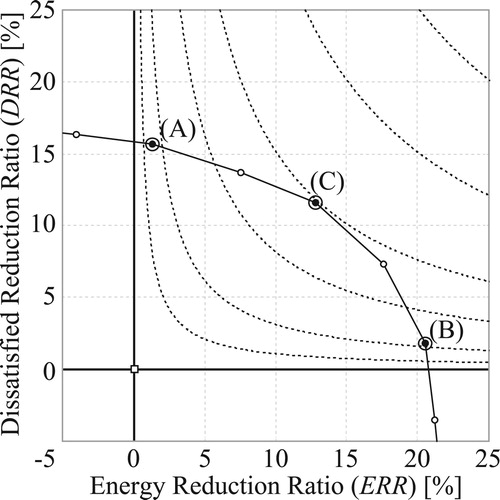
To avoid awarding high scores to operations that are extremely biased (as described above), in this paper, we awarded the total score by applying Equation (6) to calculate the effective energy reduction ratio (E2R2), which has been defined in the following section. This conditional equation adds conservativeness to the calculation of an optimal solution. Figure 2 shows several values of E2R2 plotted as contours against ERR and DRR on the x-and y-axes, respectively. Note that the value of E2R2 is zero in the second and fourth quadrants of the graph, wherein tradeoffs that ignore either comfort or energy saving exist. Moreover, the contour lines of E2R2 have ridges following the line representing ERR = DRR. Unlike a linear weighting function, E2R2 approaches zero when either indicator (ERR or DRR) approaches zero. In this manner, if an operation that neglects one index is performed, the value of E2R2 drops significantly. Figure 3 shows the pareto optimal solution with the E2R2 function. The optimal solution is (C), and it is evident from the figure that this formulation makes it more likely to ascertain approaches that can improve energy savings and comfort in a well-balanced manner, thus helping the participant to win. (6) $E2R2=\left\{\begin{array}{ll}ERR\cdot DRR& \left(0<ERR\cap 0<DRR\right)\\ 0& \left(other\right)\end{array}\right.$(6)

Figure 2. Contour lines of the Effective Energy Reduction Ratio (E2R2) function.

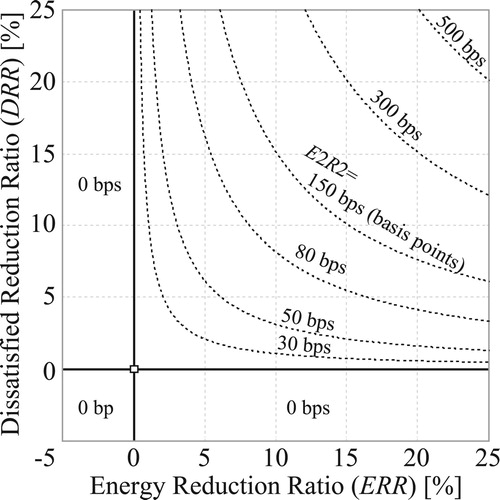
Figure 3. Pareto optimal solution with the E2R2 function.

3.2 Determination of schedule

As noted in a previous report (Togashi and Miyata 2019), we built an emulator system to remotely control the building model online using BACnet communication. However, this online approach had not been used in previous competitions, and there was a risk that limiting participation to online control only from the beginning of the championship would reduce the number of participants and, therefore, the amount of data that could be acquired. Accordingly, the championship period (from June 7th to August 7th, 2019) was divided in half, with the first and last months constituting the offline and online periods, respectively.

The offline and online periods were administered in the same manner, namely, through an emulator installed on a server. In the latter period, however, BACnet communication was allowed. The scores of the championship participants were disclosed to all participants in real time. Figure 4 shows the real-time score evaluation system.

Figure 4. Real-time score evaluation system.

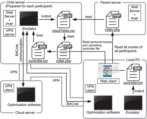
All participants were given a separate server (the Child server in Figure 4) on which the emulator was always running. When the results for one year were obtained, they were written out to the file ‘resultTable.csv.’ The collected calculation results were published by a Web server (the Parent server in Figure 4).

To start the server-side emulator calculation process, the control file (‘controller.bin’ in Figure 4) in which the control strategy (setpoint value and operation schedule) of the emulator was recorded had to be uploaded. When a participant running the emulator on a local PC controlled the settings, a control file was automatically generated. This batch-type control method is similar to the control method used by conventional energy simulation software and was therefore easy for the participants to understand; however, original feedback control using, for example, the room temperature or the behavior of the occupants inside the emulator was not possible. To perform such controls, it was necessary to connect directly to the server-side emulator online, which was permitted only during the online period in the second half of the championship.

During the online period, the participants were able to connect the emulator server via a virtual private network (VPN) that could be used for BACnet communication with the emulator. The participants could develop and run their own optimization software from either a local PC or a cloud server with a stable network to control the emulator freely.

The execution speed of the server-side emulator could be freely set by the participants and accelerated up to about 1000 times in real time. This acceleration rate could also be controlled via BACnet communication. During the offline period, a maximum acceleration rate could be set, but during the online period, the value of the acceleration rate was very important: if it was too slow, the number of challenges to improving operations would decrease; if it was too fast, the original optimization software calculations could not keep up or the communication would not be carried out in time. In other words, if excellent optimization software that operated lightly could be developed, the number of operational trials could be stably increased. Evaluation from this point of view, including the evaluation of communication stability and calculation speed, is very important when applying optimization software to real buildings.

It was expected that many participants would have no experience in developing control programs using BACnet protocol. To address this, we distributed two sample programs written in five different program languages (JavaScript (node.js), C#, Basic, C++, and Python). The first sample was titled ‘Air temperature control based on Fanger’s PMV (Fanger 1970)’ and the second sample was titled ‘Slat angle control of blinds based on solar altitude.’

3.3 Information of the participants

Table 2 lists the participants’ affiliations and job categories. Thirty-four teams had announced their participation by the deadline; one team subsequently canceled, leaving 33 teams for the final competition roster. Participants included university laboratories, corporate research institutions, designers, constructors, and managers who were interested in building operations. Some of the ‘others’ included researchers in the information technology field.

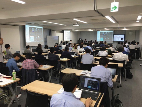
On the first day of the championship, a briefing session was held to demonstrate the use of the emulator software. It was an optional session, and 24 of 33 teams – a total of 66 people – participated. A photo of the briefing session is shown in Figure 5.

Figure 5. Scene from the briefing conducted on the first day of the Championship.

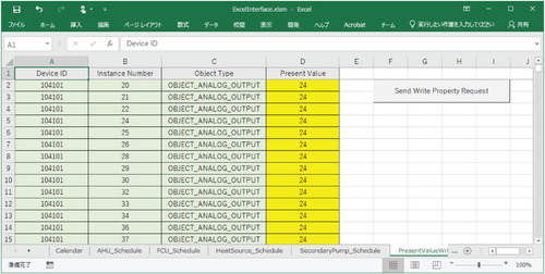
The participants in the briefing session were provided with the software shown in Figures 6 and 7, which were used to conduct a tutorial. The application in Figure 6 displays the simulation status of the emulator in real time, while that shown in Figure 7 was used to send control signals from Microsoft Excel. Both programs communicated with the emulator via BACnet. As already mentioned, the participants were free to develop their own software using BACnet, but most participants used the provided applications for optimization. The software was also distributed to teams that did not attend the briefing.

Figure 6. Emulator information display software.

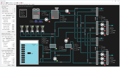
Figure 7. Emulator control software.

4. Results of the world championship of Cybernetic building optimization

4.1 Relationship between the number of calculations and scores

Figure 8 shows the number of calculation trials carried out by each team during the two-month competition period. A total of 339 calculations were performed on the server side, averaging 10.3 times per team. Team 20 carried out the most calculation trials (53), corresponding to nearly a calculation per day.

Figure 8. Number of calculation trials per team (descending order).

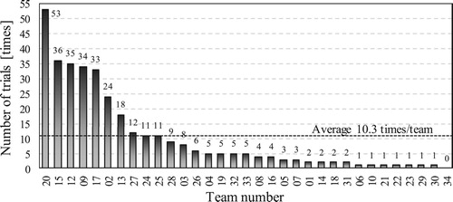
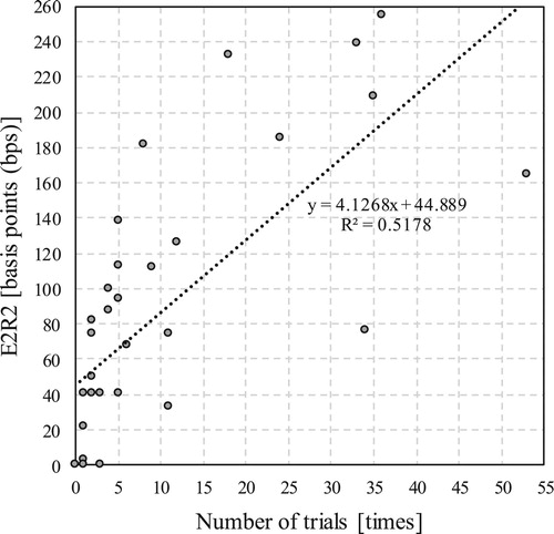
Figure 9 shows the relationship between the number of trials and the final E2R2 (comprehensive score) of each team. An interview of the four top-scoring participants after the championship revealed that each of the four teams had performed more than 50 simulations each on their local PC. An ideal building operator would attain the highest score in one simulation. However, many participants recheck the results by tuning their parameters. This suggests that building operational performance improvement can be achieved not only through inspiration but also through the application of a gradual trial-and-error process. However, it was also true that the rate of increase in the score decreased as the number of trials increased, indicating that the rate of discovery of effective measures for operational improvement decreased after repeated study of the problem.

Figure 9. Relationship between the number of trials conducted and the final E2R2 of each team.

4.2 Score changes and final results

Figure 10 shows the weekly changes in the distribution of scores over the course of the first month (offline portion) of the competition. It can be seen that the scores increased as the days pass. Initial attempts focused on increasing ERR (energy saving performance) and DRR (comfort performance) to the same extent. Later, DRR-focused operations increased in frequency, with the participants intensively searching for operating points at an ERR and a DRR of approximately 10 and 20%, respectively. Many teams with high scores operated around these points.

Figure 10. Transition of score distribution (offline period).

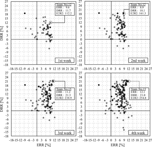
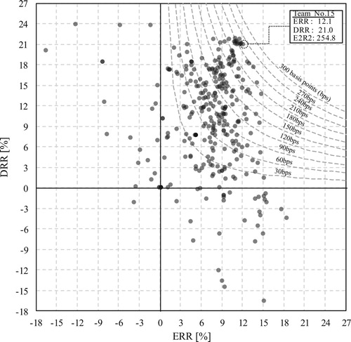
Figure 11 shows the final score distribution at the end of the online period. An examination of the modes of operation with an emphasis on energy performance confirmed that an energy reduction of up to approximately 15% was possible before the decline in comfort became too large. As it was found to be too difficult to achieve both optimal comfort and energy reduction through further adjustment, the final maximum total score was the same as that during the offline period.

Figure 11. Final score distribution.

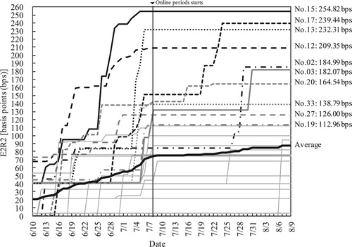
Figures 12–14 show changes in ERR (energy saving performance), DRR (comfortable performance), and E2R2 (comprehensive score) by team over the course of the championship. The x-axis denotes the date, showing the change from the start date to the end date of the championship. A vertical line is drawn at 7/7. The left side depicts the offline period, and the right side depicts the online period. Different line styles distinguish the best 10 teams, and the remaining teams are shown via light solid gray lines. As energy savings can obviously be increased by shutting off all HVAC systems while disregarding comfort, only operations at a DRR of zero or greater were used to determine the ERR ranking.

Figure 12. Changes in ERR (energy-saving performance) by team over the course of the championship.

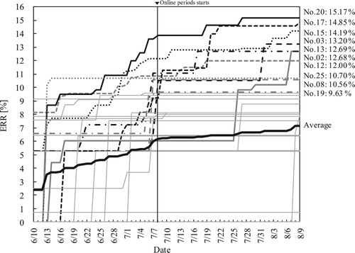
Figure 13. Changes in DRR (comfort performance) by team over the course of the championship.

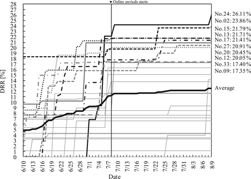
Figure 14. Changes in E2R2 (comprehensive score) by team over the course of the championship.

For all evaluation indices, no specific team was able to hold the topmost position for a long time. The participants switched their positions by raising their scores, and of course, the overall average score also increased during this process. Recall that all the scores were published on the Web in real time, allowing each participant to gauge their relative position with respect to other participants and encouraging operational improvement through competition. The change in the participants’ ranking order was intense in the offline period, but not so much in the online period. There may be three reasons for this. First, various operational improvements had already been tried and the participants were running out of new methods to test. Second, some of the lower-ranked teams decided that it was too difficult to surpass the higher-ranked teams and left the competition. In fact, some of the teams with lower scores are depicted by horizontal lines, denoting almost no change in their scores in the second half period of the competition. Third, many participants found it difficult to control the online process with BACnet. Seventeen responses were obtained from the questionnaire survey conducted after the championship. According to this survey, only 3 teams achieved online control with BACnet. Two teams failed to establish a VPN connection with the server, and the remaining 12 teams never aimed for online control.

Along these lines, a summary of the operational results of all the participants (monthly energy consumption and dissatisfaction rate of occupants) was also published on the website. According to interviews with the top teams after the championship, some participants used these summaries as benchmarks for improving their operations. The above-mentioned strategies implemented by the participants during the championship provided hints for improving the operation of real buildings. In general, no clear comparisons can be made among building operations. Therefore, even if a building is poorly operated, it is unlikely to cause much trouble, but conversely, even if a building operator were to be efficient at his task, he/she will rarely be praised. Of course, ethical operators always seek to improve their operation methods based on their personal will to do their jobs well, but their efforts are largely unrecognized. If we can reveal the results of the tuning effects made by the building operators and allow a fair comparison with similar efforts by other such practitioners, they will be encouraged to attempt further tuning. A system that enables such comparisons could be built using an emulator. We discuss this aspect in Section 5.

The final scores of the top 10 teams in terms of ERR, DRR, and E2R2 are listed in Tables 2–5, respectively. In each case, the first-ranked team is different. As energy savings and comfort share a trade-off relationship, obtaining a higher ERR or DRR ranking requires different operations. This can be evidenced by the fact that the first-ranked team in the ERR listing has a low DRR, while the first-ranked team in the DRR listing has a low ERR. Interviews with the top scorers for each ranking revealed that they performed special operations with an emphasis on one of the indicators.

Table 2. Participants’ affiliations and job categories.

No.	Affiliation	Job category	No.	Affiliation	Job category
01	Satoh Energy Research	Research	18	Tokyo Denki University	Education institution
02	Hokkaido University	Education institution	19	Anonymous	Building constructor
03	Nihon Sekkei	Building designer	20	Kanden Facilities	Building manager
04	Nagoya City University	Education institution	21	Anonymous	Other
05	Chiba University, Hayashi Laboratory	Education institution	22	Anonymous	Building designer
06	Kajima Technical Research Institute	Research	23	Anonymous	Building constructor
07	Ritsumeikan University	Education institution	24	Kogakuin University	Education institution
08	Waseda University, Tanabe Laboratory	Education institution	25	Anonymous	Building Design
09	Tokyo Polytechnic University	Education institution	26	The University of Electro-Communications, Sato Laboratory	Education institution
10	Sony CSL and Daiwa House Industry	Research	27	Anonymous	Other
11	(Canceled)	(Canceled)	28	Kansai Electric Power	Research
12	Kyushu University, Sumiyoshi Laboratory	Education institution	29	The OpenCAE Society of Japan	Other
13	Shibaura Institute of Technology	Education institution	30	Anonymous	Other
14	Anonymous	Building constructor	31	Anonymous	Research
15	Sanko Air Conditioning	Building constructor	32	Tokyo City University	Education institution
16	Anonymous	Other	33	Kansai Electric Power	Other
17	Kanden Energy Solution	Building manager	34	Anonymous	Research

Table 3. Final scores of the top 10 teams (ERR).

Rank	Team No.	Affiliation	ERR [%]	DRR [%]	E2R2 [bps]
1	20	Kanden facilities	15.17	1.31	19.99
2	17	Kanden energy solution	14.85	13.68	203.24
3	15	Sanko air conditioning	14.19	15.29	216.98
4	03	Nihon Sekkei	13.20	13.78	182.07
5	13	Shibaura Institute of Technology	12.69	11.065	147.97
6	02	Hokkaido University	12.68	9.89	125.52
7	12	Kyushu University, Sumiyoshi Laboratory	12.00	14.47	173.84
8	25	Anonymous	10.70	1.45	15.58
9	08	Waseda University, Tanabe Laboratory	10.56	6.71	70.95
10	19	Anonymous	9.63	11.72	112.96

Table 4. Final scores of the top 10 teams (DRR).

Rank	Team No.	Affiliation	ERR [%]	DRR [%]	E2R2 [bps]
1	08	Kogakuin University	−20.42	26.11	0.00
2	02	Hokkaido University	−12.20	23.86	0.00
3	15	Sanko Air Conditioning	10.94	21.79	238.49
4	13	Shibaura Institute of Technology	10.07	21.71	218.80
5	17	Kanden Energy Solution	11.18	21.41	239.44
6	27	Anonymous	4.06	20.91	85.05
7	20	Kanden Facilities	2.10	20.45	42.95
8	12	Kyushu University, Sumiyoshi Laboratory	10.44	20.05	209.35
9	33	Kansai Electric Power	7.73	17.40	134.63
10	09	Tokyo Polytechnic University	1.19	17.35	20.81

Table 5. Final scores of the top 10 teams (E2R2).

Rank	Team No.	Affiliation	ERR [%]	DRR [%]	E2R2 [bps]
1	15	Sanko Air Conditioning	12.15	20.96	254.82
2	17	Kanden Energy Solution	11.18	21.41	239.44
3	13	Shibaura Institute of Technology	11.05	21.01	232.31
4	12	Kyushu University, Sumiyoshi Laboratory	10.44	20.05	209.35
5	02	Hokkaido University	10.17	18.17	184.99
6	03	Nihon Sekkei	13.20	13.78	182.07
7	20	Kanden Facilities	8.67	18.96	164.54
8	33	Kansai Electric Power	8.03	17.27	138.79
9	27	Anonymous	7.29	17.27	126.00
10	19	Anonymous	9.63	11.72	112.97

The championship evaluated only energy savings and comfort. However, it is necessary to understand that real situations involve more complex problems, with additional trade-off indicators, which require a balance among aspects such as investment profitability, robustness, and CO₂ performance.

4.3 Score distribution

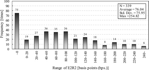
The distribution of the 339 trial scores is shown in Figures 15 and 16. The figures show that the ERR and DRR are widely distributed over both the positive and the negative ranges (with the DRR scores more widely distributed than the ERR scores), indicating a wide range of possibilities for operational improvement.

Figure 15. Frequency distribution of ERR and DRR.

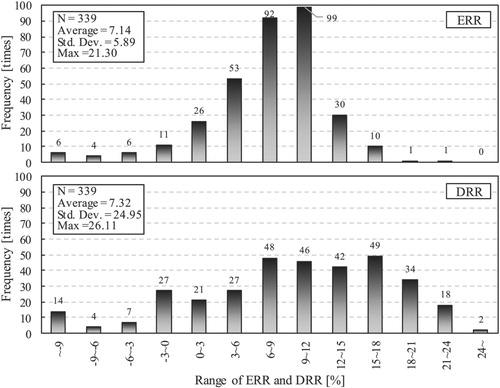
Figure 16. Frequency distribution of E2R2.

The standard deviations of ERR and DRR are approximately 6 and 25%, respectively. The performance of the hardware remained constant; thus, these distributions must have occurred due to operational differences. It was expected that the participants would not limit themselves to performing all calculations on the server and that they would additionally test operations on their local PCs. If these calculations were included in the overall analysis, the performance variability as a result of the operations would have been even greater. However, it can be assumed that the building manager of an actual building would tend to perform safe operations that consume more energy to avoid complaints from the inhabitants and, therefore, that the actual centers of distribution would be to the left and right for ERR and DRR, respectively.

As the participants in a competition of this type are expected to be primarily interested in building operations, their abilities with respect to this task would be expected to be higher than average. In reality, however, certain buildings must be operated with insufficient funds and staffing, resulting in a wider real-world distribution of operational results than those achieved in this championship.

4.4 Points to be improved

The performance evaluation revealed two points that deserve reflection.

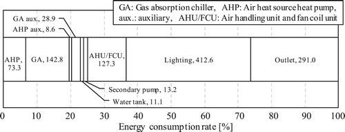
The first point regards the range over which the primary energy use was evaluated. Figure 17 shows the energy consumption rate during the default operation, which equated to an annual energy consumption of 1109 MJ/(m²·yr). While calculating ERR in Equation (3), this value was used as the standard energy consumption, E_R. The outlet and lighting energy consumption were included in this calculation to obtain a complete picture of the overall primary energy consumption by the building. This resulted in a decrease in the overall ratio of energy consumption by the HVAC component to the total consumption. As the HVAC system was the main controllable equipment in the championship, the range over which ERR could change was therefore reduced. For example, as the energy consumption by HVAC was only approximately 35% of the total, halving this consumption would only reduce ERR to 35% × 0.5 = 17.5%. Thus, the range of ERR was very limited relative to that of DRR, making the game less interesting in terms of developing a trade-off strategy. However, as blind control affects the energy consumption of both lighting and the HVAC system, lighting energy could not simply be ignored. Only the energy consumption of perimeter illumination should be summarized to evaluate the score. As the energy consumption of the outlets is a fixed value that could not be controlled, it should be neglected when evaluating the score.

Figure 17. Energy consumption rate under default operation.

Another point of reflection involves the method used for expressing uncertainty. Because the same random number seed was used during the offline periods, all the trials were performed under exactly the same weather and occupant behavior conditions. During the online periods, the control program could be complicated to an arbitrary extent, making it possible to control the weather conditions to make them fully predictable instead of (realistically) uncertain. As this would be a control overfitting to a specific condition – which is not preferable – this control was penalized during the online period by changing the random number seed each time a server-side calculation was performed. However, because the weather conditions and occupant behavior were varied with each calculation trial, it became difficult to compare the absolute values of energy consumption and dissatisfaction rate. As there were few participants who changed the online control used in the championship, it was preferable to fix the random number seed with an emphasis on the inter-compatibility of the calculation results.

In the following sections, we briefly compare the participants’ results. For a more detailed analysis, the operating data (hourly and by-minute) of all the participants can be accessed online (www.wccbo.org).

4.5 Comparison of energy consumption

Figures 18 and 19 and Table 6 show the HVAC energy consumption and consumption rate of each team under the operational conditions at which their respective E2R2 ratings obtained the maximum value.

Figure 18. Primary HVAC energy consumption by team.

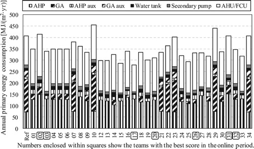
Figure 19. Primary HVAC energy consumption rate by team.

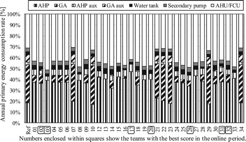
Table 6. Primary HVAC energy consumption obtained by each team [MJ/(m²·yr)].

No.	AHP	GAR	AHP auxiliary	GAR auxiliary	Water tank pump	Secondary pump	AHU/FCU
Ref.	73.2	143.6	8.6	28.8	11.1	13.2	127.3
01	128.7	23.5	18.1	2.5	11.6	14.1	150.2
02	149.3	34.8	15.3	3.1	11.7	14.3	184.8
03	130.8	0.0	13.7	0.0	8.2	11.9	173.5
04	128.7	23.5	18.1	2.5	11.6	14.1	150.2
05	128.7	23.5	18.1	2.5	11.6	14.1	150.2
06	128.7	23.5	18.1	2.5	11.6	14.1	150.2
07	75.2	129.5	7.5	26.2	10.9	12.9	117.1
08	140.0	0.0	21.9	0.0	6.3	16.8	176.2
09	121.4	25.3	17.7	3.1	12.4	13.9	139.8
10	75.9	160.8	8.7	31.4	11.3	14.8	150.6
12	124.1	2.4	14.9	0.3	12.9	11.5	132.1
13	120.2	0.0	15.4	0.0	13.3	13.2	136.9
14	103.3	21.8	15.1	2.3	16.5	9.5	155.3
15	121.1	0.0	14.7	0.0	14.0	7.3	130.3
16	138.5	7.6	19.9	0.6	3.6	9.7	160.5
17	130.6	0.0	19.9	0.0	4.8	6.3	117.2
18	115.2	27.2	15.8	2.2	13.1	13.3	148.2
19	117.8	0.0	14.3	0.0	14.4	9.0	145.0
20	124.2	0.0	15.9	0.0	10.1	13.0	146.9
21	75.2	107.2	8.4	17.4	10.5	7.9	108.8
22	73.2	121.2	8.6	20.9	11.1	12.3	115.3
23	71.5	141.4	8.6	27.6	10.4	13.3	128.5
24	118.6	18.0	14.9	2.0	10.8	12.3	142.8
25	108.0	9.1	14.9	1.5	10.3	12.3	138.1
26	111.2	17.2	17.5	1.8	7.5	14.3	163.2
27	143.5	0.0	19.1	0.0	11.4	9.2	147.9
28	119.9	19.8	18.3	1.2	4.5	14.5	139.0
29	75.5	153.9	8.8	28.6	11.4	14.3	148.8
30	119.0	24.3	17.3	2.7	14.1	13.6	145.8
31	152.0	38.1	17.6	3.5	10.0	14.0	171.9
32	127.6	25.0	16.9	2.2	10.8	13.9	149.0
33	130.5	0.0	15.8	0.0	7.8	9.1	154.8
34	73.2	143.6	8.6	28.8	11.1	13.2	127.3

GA: Gas absorption chiller, AHP: Air heat source heat pump, AHU/FCU: Air handling unit and fan coil unit.

Two major groups are apparent: teams that prioritized the air heat-source heat pump and teams that prioritized the direct absorption chiller/heater. The top three teams – Nos. 3, 17, and 15 – did not operate any direct absorption chiller/heater at all, and instead produced all the heat by using an air source heat pump. As there were no tenants on the third floor of the office building to be optimized, and the schedule of activities was different for each tenant, no design peak load occurred.

The energy consumption of the heat charge/release pump of the water heat storage tank varied considerably by team. It seems likely that the team with the highest score extended the operating time of the air source heat pump by changing the schedule using the water heat storage tank.

While many teams increased the energy consumption of the air handling unit to above the baseline, team No. 17 reduced it. An interview with this team revealed that they reduced the operating time of the air handling units in accordance with the activities of the respective tenants.

Team Nos. 15 and 17 succeeded in halving the energy consumption of the secondary pump. Among the top performing teams, they were the only ones who adjusted the parameters of the formula that estimated the required differential pressure of the secondary pump.

4.6 Comparison of thermal comfort

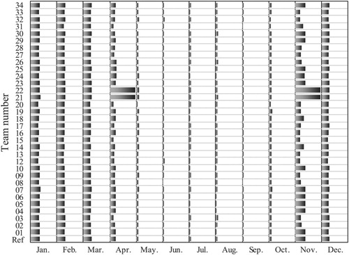
Figure 20 shows the monthly dissatisfaction rate (as a percentage) obtained by each team at their respective maximum E2R2 value. In the winter, the dissatisfaction percentage is much higher and the variation among the teams is greater than in the summer. One reason for this is that upon starting up in the morning, the thermal environment is more extreme during the winter because the building structure becomes very cold during the night. Furthermore, the heating mode applied during winter mornings must be switched to a cooling mode during the afternoon, but it is difficult to set the timing for this mode switching. Teams 21 and 22 tried to spend the warm mid-season (Apr. and Nov.) with only ventilation and no air conditioning; however, the dissatisfaction percentage became extremely high, and they failed the task (Figure 21).

Figure 20. Monthly dissatisfaction percentage by team at maximum E2R2.

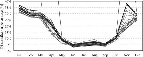
Figure 21. Total number of dissatisfied occupants by team.

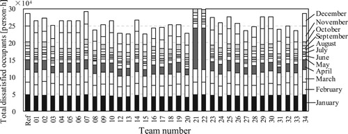
Figure 22 shows the monthly dissatisfaction percentage obtained by each team. The variation was the greatest in November, followed by April, suggesting that the quality of these mid-season operations had a significant effect on the final scores. The highest-scoring teams – Nos. 12, 15, and 17 – had clearly lower dissatisfaction percentages than the other teams during winter months such as January and February.

Figure 22. Monthly dissatisfaction percentage by team.

5. Conclusion

In this paper, we reported the results of a championship in which teams competed to optimize building operation performance using an emulator.

A review of the history of similar open championships reveals that they promote the development of new technologies and skills through competition. During our championship, it was evident that a number of participants improved their operational performance competitively based on the monitoring of other teams’ scores. Current building operation processes are not actually competitive, and the operational management process generally differs from one building to another. To improve operations by introducing the element of competition, it is necessary to compare the performance in some concrete manner. Such comparison has been conventionally difficult because buildings are generally standalone entities; however, the development of simulation technologies is making it possible to operate buildings virtually. With the spread of building information modeling in recent years, the concept of ‘digital twinning,’ wherein a building that behaves exactly like a real building is constructed in cyberspace, has been increasingly studied (Lydon et al. 2019; Kaewunruen, Rungskunroch, and Welsh 2018). In the future, digital twins should be designed with the purpose of virtualizing building operation. If virtual operation becomes possible with a digital twin, as described below, there exists a possibility that building operation services can be traded in an ideal competitive market, or free market.

Allowing for the control of such systems using BACnet communication and VPN, as was done in our championship, would enable building operations that are not restricted by location. Currently, building operations are usually carried out continuously by specific building managers, but the use of systems such as that in our championship would make it possible to replace operators dynamically. In other words, it would enable an approach wherein a number of operator candidates parallelly perform operations on a virtual building with a network of operators that achieved the best empirical scores with an actual building. In digital twinning, a virtual building that shows exactly the same response as a real building exists in parallel on the network. In fact, because these buildings can be replicated innumerable times, it may be better to call them ‘digital clones’ rather than digital twins. When switching operators, as described above, the compensation for operating the building could be paid according to the connection time to the real-world building. If such a mechanism could be established, building operation services could be traded in a completely competitive market. As operators who can propose a good building operation strategy at a lower cost are more competitive, service providers will begin to develop software that automatically provides superior operational strategies at low cost based on machine learning and other techniques. An emulator can express uncertainties in building parameters, which is useful to check the performance of machine learning. Emulators can also be replicated as needed, making them invaluable as models for reinforcement learning. Meanwhile, from the demand side perspective, owners who pay higher compensation can secure the services of more skilled building operators.

For the purposes of this championship, the authors developed all the models from scratch. However, if the service described above is to be realized, it is necessary to further improve the ability of the models to mimic real-world conditions. To do this, the emulator should be divided into components, and the device model should be provided by the manufacturer. In this case, model-based development (e.g. Modelica) would be a powerful tool (IEA 2017; Wimmer et al. 2015; Kim et al. 2015; Pinheiro et al. 2018). Providing equipment models, however, constitutes a new burden for manufacturers. Nonetheless, more information will be available on how these models should be used in the operational stage, undoubtedly driving technological progress.

Our championship was also useful in that it clarified the potential value of building operations. Maintaining a building in a comfortable manner while saving energy requires both good hardware and proper operational procedures. However, because buildings are single-product installations, it is conventionally impossible to know exactly what may happen if one were operated in a manner that differed from reality. The results of this championship revealed the wide differences in operational effectiveness, even among practitioners who are more competent and better trained than the general population. We also found that the participants tended to improve their scores by repeating operational procedures. It should be emphasized that the observed differences in scores were purely the result of operational factors, as the HVAC hardware was exactly the same for all the participants. Repeating competitions such as ours will allow a more quantitative evaluation of the potential value of operational ability, which in turn will contribute to maximizing the value of buildings over their entire life cycle, including the operational stage.

As mentioned already, all the operational data recorded by each participant in this championship are available on the website. Also, since all the emulator systems (including the source code) can be downloaded, interested readers and practitioners are welcome to attempt virtual operations and evaluate their tuning abilities. Since the source code was released under the General Public License, our emulator is free and open to modification, and we hope that improved versions will be developed in the future.

Acknowledgements

This research was conducted as part of the activities of the ‘Air Conditioning Equipment Committee' at ‘The Society of Heating, Air-Conditioning and Sanitary Engineers of Japan.' We would like to thank all the participants of the championship.

Disclosure statement

No potential conflict of interest was reported by the author(s).

Additional information

Funding

This work was supported by JSPS KAKENHI [grant numbers JP 16K18198 and JP 18K04462].

References

- Bushby, S. T., N. Castro, M. A. Galler, and C. Park. 2001. “Using the Virtual Cybernetic Building Testbed and FDD Test Shell for FDD Tool Development.” National Institute of Standard and Technology: NISTIR 6818.
- Bushby, S. T., N. M. Ferretti, M. A. Galler, and C. Park. 2010. “The Virtual Cybernetic Building Testbed – A Building Emulator.” ASHRAE Transactions 116 (1): 37–44.
- Chau, C. K., T. M. Leung, and W. Y. Ng. 2015. “A Review on Life Cycle Assessment, Life Cycle Energy Assessment and Life Cycle Carbon Emissions Assessment on Buildings.” Applied Energy 143: 395–413. doi:10.1016/j.apenergy.2015.01.023.
- Chonan, Y., K. Nishida, and T. Matsumoto. 1996. “A Bayesian Non-Linear Regression with Multiple Hyperparameters on the ASHRAE II Time Series Data.” ASHRAE Transactions 102 (2): 405–411.
- CIBSE (The Chartered Institution of Building Services Engineers). 2015. Building Performance Modelling CIBSE AM 11. 2nd ed.
- Dodier, R., and G. Henze. 1996. “A Statistical Analysis of Neural Networks as Applied to Building Energy Prediction.” In Proceedings of the 1996 ASME/JSME International Solar Energy Conference, 495–506.
- Fanger, P. O. 1970. Thermal Comfort – analysis and Applications in Environmental Engineering. Copenhagen: Danish Technical Press.
- Feuston, B. P., and J. H. Thurtell. 1994. “Generalized Non-Linear Regressions with Ensemble of Neural Nets: The Great Energy Predictor Shootout.” ASHRAE Transactions 100 (2): 1075–1080.
- Haberl, J., and S. Thamilseran. 1996. “Predicting Hourly Building Energy Use: The Great Energy Predictor Shootout II: Measuring Retrofit Savings – Overview and Discussion of Results.” ASHRAE Transactions 102 (2): 419–435.
- IEA (International Energy Agency). 1997. “ Energy Conservation in Buildings and Community Systems Programme (ECBCS).” Summary of IEA Annexes 16 and 17, Annex 17 – Building Energy Management Systems (BEMS) – Evaluation and Emulation Techniques.
- IEA (International Energy Agency). 1999. Energy Conservation in Buildings and Community Systems Programme (ECBCS). Annex 25 –Real Time Simulation of HVAC Systems for Building Optimization, Fault Detection and Diagnostics.
- IEA (International Energy Agency). 2008. Worldwide Trends in Energy Use and Efficiency. Connecticut: Turpin Distribution.
- IEA (International Energy Agency). 2017. Energy in Buildings and Communities Programme (ECB). IEA Annexes 60 Final Report – New Generation Computational Tools for Building & Community Energy Systems.
- Iijima, J., K. Takagi, R. Takeuchi, and T. Matsumoto. 1994. “A Piecewise – Linear Regression on the ASHRAE Time Series Data.” ASHRAE Transactions 100 (2): 1088–1095.
- Jang, K.-J., E. Bartlett, and R. Nelson. 1996. “The Great Energy Predictor Shootout II: Measuring Retrofit Energy Savings Using Autoassociative Neural Networks.” ASHRAE Transactions 102 (2): 412–418.
- Kaewunruen, S., P. Rungskunroch, and J. Welsh. 2018. “A Digital-Twin Evaluation of Net Zero Energy Building for Existing Buildings.” Sustainability 11: 159. doi:10.3390/su11010159.
- Katipamula, S. 1996. “The Great Energy Predictor Shootout II: Modeling Energy use in Large Commercial Buildings.” ASHRAE Transactions 102 (2): 397–404.
- Kawashima, M. 1994. “Artificial Neural Network Backpropagation Model with Three-Phase Annealing Developed for the Building Energy Predictor Shootout.” ASHRAE Transactions 100 (2): 1096–1103.
- Khoury, J., Z. Alameddine, and P. Hollmuller. 2017. “Understanding and Bridging the Energy Performance gap in Building Retrofit.” Energy Procedia 122: 217–222. doi:10.1016/j.egypro.2017.07.348.
- Kim, J. B., W. Jeong, M. J. Clayton, J. S. Haberl, and W. Yan. 2015. “Developing a Physical BIM Library for Building Thermal Energy Simulation.” Automation in Construction 50: 16–28. doi:10.1016/j.autcon.2014.10.011.
- Kreider, J. F., and J. S. and Haberl. 1994. “Predicting Hourly Building Energy Use: The Great Energy Predictor Shootout – Overview and Discussion of Results.” ASHRAE Transactions 100 (2): 1104–1118.
- Lebrun, J., and S. W. Wang. 1993. “Evaluation and Emulation of Building Energy Management Systems – Synthesis Report, IEA Annex 17 Final Report.” Belgium: University of Liege.
- Lydon, G. P., S. Caranovic, I. Hischier, and A. Schlueter. 2019. “Coupled Simulation of Thermally Active Building Systems to Support a Digital Twin.” Energy & Buildings. doi:10.1016/j.enbuild.2019.07.015.
- MacKay, D. 1994. “Bayesian Non-Linear Modeling for the Energy Predictor Competition.” ASHRAE Transactions 100 (2): 1053–1062.
- Mohammed, T., R. Greenough, S. Taylor, L. Ozawa-Meida, and A. Acquaye. 2013. “Operational vs. Embodied Emissions in Buildings – a Review of Current Trends.” Energy and Buildings 66: 232–245. doi:10.1016/j.enbuild.2013.07.026.
- Nguyen, A., S. Reiter, and P. Rigo. 2014. “A Review on Simulation-Based Optimization Methods Applied to Building Performance Analysis.” Applied Energy 113: 1043–1058. doi:10.1016/j.apenergy.2013.08.061.
- Ohlsson, M., C. Peterson, H. Pi, T. Rognvaldsson, and B. Soderberg. 1994. “Predicting Utility Loads with Artificial Neural Networks – Methods and Results From ‘The Great Energy Predictor Shootout.’.” ASHRAE Transactions 100 (2): 1063–1074.
- Ono, E., S. Ito, and H. Yoshida. 2017. “Development of Test Procedure for the Evaluation of Building Energy Simulation Tools.” Proceedings of the International Building Performance Simulation Association, 380–388. doi:10.26868/25222708.2017.10z.
- Pinheiro, S., R. Wimmer, J. O’Donnell, S. Muhic, V. Bazjanac, T. Maile, J. Frisch, and C. Treeck. 2018. “MVD Based Information Exchange Between BIM and Building Energy Performance Simulation.” Automation in Construction 90: 91–103. doi:10.1016/j.autcon.2018.02.009.
- Rouchier, S. 2018. “Solving Inverse Problems in Building Physics: An Overview of Guidelines for a Careful and Optimal use of Data.” Energy & Buildings 166: 178–195. doi:10.1016/j.enbuild.2018.02.009.
- Rumelhart, D. E., G. E. Hinton, and R. J. Williams. 1986. “Learning Representations by Back-Propagating Errors.” Nature 323 (6088): 533–536. doi:10.1038/323533a0.
- Sartori, I., and A. G. Hestnes. 2007. “Energy Use in the Life Cycle of Conventional and Low-Energy Buildings.” Energy and Buildings 39: 249–257. doi:10.1016/j.enbuild.2006.07.001.
- SHASE (Society of Heating, Air-Conditioning and Sanitary Engineers of Japan). 1998. “Research on Fault Diagnosis and Optimization of Heat Storage HVAC System (in Japanese).” Final Report of Committee of Heat Storage Optimization.
- SHASE (Society of Heating, Air-Conditioning and Sanitary Engineers of Japan). 2016. “SHASE-G 1008-2016, Guideline of Test Procedure for the Evaluation of Building Energy Simulation Tool.”
- Stevenson, W. J. 1994. “Predicting Building Energy Parameters Using Artificial Neural Nets.” ASHRAE Transactions 100 (2): 1081–1087.
- Togashi, E., and M. Miyata. 2019. “Development of Building Thermal Environment Emulator to Evaluate the Performance of the HVAC System Operation.” Journal of Building Performance Simulation. doi:10.1080/19401493.2019.1601259.
- Togashi, E., and S. Tanabe. 2009. “Methodology for Developing Heat-load Calculating Class Library with Immutable Interface.” Technical Papers of the Annual Meeting of the Society of Heating, Air-conditioning and Sanitary Engineers of Japan, 1995–1998. doi:10.18948/shasetaikai.2009.3.0_1995.
- Vaezi-Nejad, H., E. Hutter, P. Haves, A. L. Dexter, G. Kelly, P. Nusgens, and S. W. Wang. 1991. “The Use of Building Emulators to Evaluate the Performance of Building Energy Management Systems.” In Proceedings of Building Simulation 1991 Conference, 209–213.
- Wilde, P. 2014. “The Gap Between Predicted and Measured Energy Performance of Buildings: A Framework for Investigation.” Automation in Construction 41: 40–49. doi:10.1016/j.autcon.2014.02.009.
- Wimmer, R., J. Cao, P. Remmen, and T. Maile. 2015. “Implementation of Advanced BIM-Based Mapping Rules for Automated Conversions to Modelica.” Proceedings of BS2015: 14th Conference of International Building Performance Simulation Association, 7–9.
- Zhang, Y., Y. Zhang, W. Shi, R. Shang, R. Cheng, and X. Wang. 2015. “A new Approach, Based on the Inverse Problem and Variation Method, for Solving Building Energy and Environment Problems: Preliminary Study and Illustrative Examples.” Building and Environment 91: 204–218. doi:10.1016/j.buildenv.2015.02.016.