An open source analysis framework for large-scale building energy modeling

Abstract

Full integration of building energy modelling into the design and retrofit process has long been a goal of building scientists and practitioners. However, significant barriers still exist. Among them are the lack of available: (1) configurable technology stacks for performing both small- and large-scale analyses, (2) different classes of algorithms compatible with common design workflows, and (3) analysis tools for effectively visualizing large-scale simulation results. This article discusses the OpenStudio® Analysis Framework: a scalable analysis framework for building energy modelling that was developed to overcome the three barriers listed above. The framework is open-source and scalable to facilitate wider adoption and has a clearly defined application programming interface upon which other applications can be built. It runs on high-performance computing systems, within cloud infrastructure, and on laptops, and uses a common workflow to enable different classes of algorithms. Lessons learned from previous development efforts are also discussed.

KEYWORDS:

• Parametric analysis
• optimization
• calibration
• sensitivity analysis
• uncertainty quantification
• OpenStudio Analysis Framework

1. Introduction

As detailed in Hong, Langevin, and Sun (2018), the full integration of building energy modelling (BEM) into the building design and retrofit process has been a long-term goal of many building scientists and practitioners. In the ideal case, potential improvements to buildings could be quickly evaluated based on their impact on various metrics, such as energy consumption, life cycle cost, peak demand, indoor environmental quality (including thermal and visual comfort), and greenhouse gas emissions. However, calculating such metrics is time-consuming and computationally intensive. To generate these metrics, a practitioner needs access to a computing platform that is easily configurable as well as computing resources that can scale to the problem being solved. To conduct a thorough analysis in a realistic timeframe, practitioners need access to various algorithms to perform sensitivity analyses, uncertainty quantification, design optimization, and model calibration. These algorithms should be easily configurable and effortlessly interchangeable without having to completely reformulate the problem. In this article, the term ‘algorithm’ is used to describe a process that is completely external to the building energy model and operates across multiple model runs, as opposed to an internal computation (such as how short wave radiation is applied to zone surfaces, for example).

As reported in Gestwick and Love (2014), practitioners outside of a research environment are unlikely to have the resources needed to create a robust computing system with the capabilities to manage and schedule multiple simulation runs, also called batch processing. Because of this, the authors and many similar practitioners generally restrict their work to quick running, but less detailed models (such as DOE-2 models; see Winkelmann et al. 1993) with ad hoc workarounds to handle the lack of readily available analysis capability. As an example, Nguyen and Reiter (2015) compared various sensitivity analysis methods without an efficient simulation framework. The work took the authors 10 consecutive days to run only 8,968 simulations, with each model having a mere 2-minute runtime. Similarly, Tian (2013) highlighted the following two examples where the lack of a scalable simulation framework hindered BEM analyses: (1) Tian and de Wilde (2011) resorted to using idle campus desktop computers networked together to run 2,400 simulations in a full day. (2) Eisenhower et al. (2012) used a 184-CPU Linux computing cluster, which is a set of connected computers, to run 5,000 models. Nguyen, Reiter, and Rigo (2014) also suggest that the lack of easy-to-use large-scale computing platforms hinders optimization of building energy models and forces some users to use simplified models – such as reduced-order or surrogate models – instead of more detailed models, thus sacrificing accuracy for computational speed. Creating computing resources to perform even the simplest of analyses is a major barrier for typical BEM practitioners. Compounding this is the fact that BEM projects have evolved over the last decade from being relatively simple batch run simulations to more advanced analyses requiring iterative optimization and calibration algorithms.

Analyzing the results of large-scale parametric BEM analyses, which are simulation-based experiments designed to characterize relationships between different model parameters and outputs, is also a formidable challenge (Jabi 2016). The rising popularity of machine learning and artificial intelligence has produced several commercially and freely available analysis and business intelligence software tools (e.g. Microsoft Power BI, Dundas BI, IBM Cognos Analytics), and several companies have business models based around providing analysis tools and business intelligence as services. However, integrating these platforms with BEM data can require extensive post-processing to translate the data to suitable formats. Hong, Langevin, and Sun (2018) explain that merging BEM results with business intelligence tools such as machine learning and artificial intelligence is an important future direction for the industry.

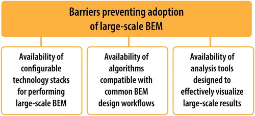
Many tools and user interfaces have been created for BEM since 2010, with more than 198 identified by the International Building Performance Simulation Association (IBPSA-USA 2019). However, basic adoption barriers remain, including the availability of: (1) configurable technology stacks for performing large-scale BEM, (2) algorithms compatible with BEM design workflows, and (3) analysis tools for effectively visualizing large-scale results. Several of the tools identified by IBPSA can overcome one or two of these barriers but are unable to overcome all three.

This article first provides a brief background (Section 2) of various BEM applications and workflows to provide lessons learned in the design and implementation of large-scale BEM simulation platforms. We then introduce the OpenStudio Analysis Framework (OSAF), which is the culmination of many of these previous attempts to create a workflow with the intention of addressing the three adoption barriers, depicted in Figure 1, in a single framework. The architecture, building blocks, and technical logistics of OSAF are detailed in Section 3. We present case studies to demonstrate specific capabilities and use cases to show the functionality of OSAF in Section 4. Finally, in Section 5 we conclude with potential future applications for OSAF.

Figure 1. Barriers to adoption of large-scale BEM analysis. Marjorie Schott, National Renewable Energy Laboratory.

2. Background

2.1. Early development of large-scale BEM technology stacks

In 2003, large-scale parametric analyses¹ of EnergyPlus® simulations (Crawley et al. 2001) became possible and peaked at around 100,000 simulations per analysis (Griffith et al. 2006). EnergyPlus runtime was significantly longer than other modelling tools at the time, such as DOE-2, but the increased runtime was deemed acceptable because EnergyPlus was designed to handle more complex building interactions across the various building domains (Crawley et al. 2008). The results of these analyses were post-processed using relational databases, Microsoft Excel, Interactive Data Language (see L3 Harris Geospatial 2020), and MATLAB.

Once parametric analyses could be run for EnergyPlus, the next evolutionary step was to add optimization capabilities and more advanced data visualizations. BEopt™ (Christensen et al. 2006) and Opt-E-Plus (Long et al. 2010) provided these new capabilities and were developed for researchers and practitioners. Opt-E-Plus, designed to be the commercial building equivalent of the residential focused BEopt, ran a greedy sequential search algorithm with inputs consisting of high-level continuous and discrete variables such as aspect ratio, square footage, and window-to-wall ratio. The iterative algorithm continued until various stopping criteria were met. The result was a cost/energy Pareto frontier. The enabling technology of Opt-E-Plus and the parametric/optimization analyses was a software tool called the XML Preprocessor (Griffith et al. 2008). The XML Preprocessor was an input file specified in eXtensible Markup Language (XML) that allowed the user to edit high-level data, such as number of floors; building layout; and heating, ventilating, and air-conditioning (HVAC) system types. The ability to define buildings at a higher level was useful because it let the user model a larger number of building designs without needing to directly edit EnergyPlus input files, which is a tedious and often error-prone task.

The EnergyPlus Example File Generator (2013) was developed a few years later based on the Opt-E-Plus software stack. It allowed practitioners to quickly generate an EnergyPlus model by entering very high-level and limited details into a web-based form. The simulation was run on a remote server, and results were sent to the user upon completion. This system attempted to address the lack of access to appropriate computing resources. The OpenStudio SketchUp Plug-in (Ellis, Torcellini, and Crawley 2008; Roth 2017) was also developed around the same time as the EnergyPlus Example File Generator and was designed to aid in the generation of more detailed and complex building geometry for EnergyPlus models.

Although these software tools added significantly to a practitioner's modelling capabilities, many limitations remained. Overall, the new portfolio of tools was disparate, with limited interoperability between tools. The XML Preprocessor could only access modelling objects at a high level (e.g. floor layout, number of floors, window-to-wall ratio, HVAC system types), and although making custom geometry was possible, it was particularly challenging. Opt-E-Plus only worked on Microsoft Windows. Additionally, the code to simulate the various energy saving technologies (now called energy conservation measures or energy efficiency measures) was compiled directly into the source code and were difficult to modify and verify. The building energy codes and standards implemented within Opt-E-Plus were also hard-coded into the software and required significant user knowledge to extend when new codes and standards became available. The EnergyPlus Example File Generator had even more restrictions on model manipulation and was not very adaptable. The combination of increasingly complex building science analysis needs coupled with software solutions that were difficult to manage and/or extend led to the develop of the OpenStudio Software Development Kit (SDK) (OpenStudio Development Team 2017). The OpenStudio SDK was designed to provide generic access to scripted modelling for various tools via application programming interface (API) access, which is a set of functions that defines how to access and use an application (Guglielmetti, Macumber, and Long 2011; OpenStudio Development Team 2019).

As work continued on the OpenStudio SDK in the early 2010s to increase the interoperability among EnergyPlus-based applications, other free (often open source) parametric and optimization tools with user interfaces were developed to evaluate and improve building design alternatives by running parametric designs and optimizations (Attia et al. 2013). Until the late 2000s, most tools directly manipulated the input formats of BEM engines. For example, one of the pioneers of merging BEM and optimization, GenOpt (Wetter 2001), allowed text substitution for any text-based engine. However, the tool did not support algorithms that optimize more than one objective function, called multi-objective optimization, and parallelization on distributed computing systems, a necessary capability to reduce the computation time of large-scale analyses, remained a challenge. jEPlus (see jEPlus + EA 2011) began development around the same time as Opt-E-Plus and was freely available. It provided a limited set of text substitution optimization-based analyses. Both GenOpt and jEPlus lacked built-in tools for effective visualization of results.

All the tools presented in this section advanced the utility and capability of BEM. However, several challenges consistently presented themselves during development. They include the ability to: (1) perform large-scale BEM, (2) easily move a defined BEM design workflow from one algorithm type to another, and (3) effectively visualize and post-process large-scale output data.

2.2. Inception of the OpenStudio high-Performance computing framework

The OpenStudio SDK enabled several workflows, including model generation, codes and standards work, optimization, and high-level object manipulation. To support different projects over the years, multiple algorithmic/analysis framework implementations were considered, including leveraging the scientific computing software package DAKOTA (Adams et al. 2009) to support optimizations and using the computer language CLIPS (Giarratano 2002) to evaluate rulesets for codes and standards.

In 2012, the U.S. Department of Energy began developing the infrastructure underpinning the Building Energy Asset Score, which is the national asset rating system for commercial buildings (Long, Goel, and Horsey 2015; Wang et al. 2018). The Building Energy Asset Score tool uses the OpenStudio SDK for model generation and articulation. However, the existing OpenStudio SDK did not support the large number of simulations needed for parameter sensitivity analyses and thus could not perform parametric analysis tasks such as properly determining the distribution of energy use intensity across the multidimensional input parameter space. At that time, OpenStudio did not support a distributed workflow and a centralized collection of results for analysis and visualization, which prevented scalability. To effectively complete a national-scale analysis such as the one required by Building Energy Asset Score, a larger management database referred to here as ‘server’, that allowed concurrent connections to store analysis data from multiple processors, referred to here as ‘workers’, running on remote hardware was needed. OpenStudio's existing database solution was SQLite (2012), and it did not support the desired distributed workflow because it did not support concurrent write access from multiple networked processes. OpenStudio's original analysis capabilities were implemented in C++, within the OpenStudio SDK. Because C++ is a compiled language, rapid development was prevented because of the long iteration cycles required to make changes as well as the significant programming expertise required to make those changes. Because the Building Energy Asset Score timeline was short and required running on institute-owned supercomputing resources, development of the OpenStudio high-performance computing (HPC) framework began as a separate project from the SDK. This was a key design decision to move the SDK away from a monolithic architecture and toward a more modular approach to the software development of the analysis framework.

In 2013, the OpenStudio HPC framework defined energy conservation measures using a structured spreadsheet format (Long and Ball 2016). An ordered group of spreadsheet rows defined the energy conservation measure and its associated variables. Each measure was implemented as a simple script that modified the Building Energy Asset Score's XML input file. The arguments to the script could also be turned into variables. Each energy conservation measure variable could be given a default value, a probability distribution, or a discrete set of values. The Ruby programming language was used to parse the spreadsheet and pass the data to the statistical programming language R (R Core Team 2017) to generate variable distributions and subsequently produce the entire multidimensional parameter space using Latin hypercube sampling. Each point in the parameter space was mapped to the energy conservation measure variables and simulations were run with a new programme called the OpenStudio Workflow Gem (OpenStudio Development Team 2014). The Workflow Gem was OpenStudio's first attempt at standardizing a BEM-based energy conservation measure and design workflow – thus making it compatible with scientific software packages, as discussed in Section 3.4 – and distributing it as a compiled library using methods adapted from the open-source software development community.

Using the OpenStudio HPC framework, the Building Energy Asset Score study ran ∼350,000 simulations per analysis on Red Mesa, a supercomputer at Sandia National Laboratories. The implementation worked well, but the software dependency management required significant manual configuration, access to the supercomputer, and reliance on supercomputer batch run schedulers. The framework had evolved from being difficult to develop but easy to run, to a system that was easier to comprehend and modify but limited by the specialized configuration and resources – therefore, still difficult to use.

The technological advances discussed in this section were distributed to the BEM community as open-source software, but practical large-scale BEM was still not widespread enough to significantly impact energy efficiency in buildings. The skills and equipment necessary to perform the relevant analyses were still limited to building researchers and academics. These shortfalls motivated the development of an updated framework, now called the OpenStudio Analysis Framework (OSAF). The intent of OSAF was to create a framework that was simple to develop, extend, deploy, and use (by non-research-based design professionals) by relying on the now easily accessible internet-hosted cloud-based servers instead of institute-owned HPC resources.

2.3. Virtual machines and OpenStudio server

A common challenge of software projects is managing the software development life cycle (Merkel 2014); more specifically, managing the development, testing, and deployment of new code at any interval in the cycle. Traditionally, most BEM software tools are available only for a single platform (typically Microsoft Windows). The desire to move to large-scale analysis requires the software to be built for other platforms (specifically Linux-based operating systems) to take advantage of HPC and the emerging cloud-based resources. EnergyPlus became available for Linux platforms in the early 2000s, which allowed for batch parallelization on HPC clusters.

To address the barrier of availability of configurable technology stacks for performing large-scale BEM, the ability to perform large-scale analyses both locally on various platforms and remotely on HPC or cloud infrastructure was the next challenge to focus on. Virtual machines, which are an emulation of a computer system, were used to address the local/remote challenge on various platforms (Windows, Mac, and Linux), and the resulting software stack was called OpenStudio Server (Long et al. 2014). The workflow to automatically create, test, and deploy new virtual machines was cumbersome, but it allowed an inexperienced user to create a computing cluster in the cloud that could run tens of thousands of simulations. Running the same workflow locally required a more advanced user who was familiar with managing virtual machines, but it was possible and often done during in-house development and testing of capabilities and features.

The uniformity in the software stack made possible by using virtual machines allowed the software to become more robust and powerful in handling queuing of simulations, parallelization, advanced parametric and optimization algorithms, visualization, and logging, while maintaining simplicity in the development life cycle. The goal of building the application once and easily deploying it across a wide range of environments was nearly achieved, except for the more complex HPC platforms. However, using virtual machines led to several issues, including slow start times (on the order of tens of minutes), slow generation of new virtual machines (on the order of many hours), required segmenting of system resources, difficulty in managing clusters, and the inability to run easily on HPC nodes. The virtual machine approach also did not scale as was hoped, because of the inherent overhead of the technology and excessive disk input/output that grew as the size of the virtual machine increased.

3. Methods

3.1. Docker and containerization

In 2013, a tool called Docker was officially released (Merkel 2014). Docker enables the use of Linux containers, which are combinations of software code and dependencies in a lightweight and standalone package that includes everything needed to run an application. Containers can be used together and are designed to work in a networked environment across different computers. Docker containers also use less disk space than virtual machines because containers share the host operating system's kernel, as opposed to virtual machines that must provide their own full copy of an operating system.

OSAF is made up of two Docker containers that are hosted on Docker Hub for ease of installation (OpenStudio Development Team 2020). The first is the OpenStudio-Rserve container, which provides access to the R parametric and optimization algorithms as a service and is discussed in Section 3.3. The second is the OpenStudio-Server container, which provides the front-end graphical user interface and manages the back-end communications for the entire OSAF. It also contains the database, the queue, and all the BEM-related software, including EnergyPlus. The OpenStudio-Server container is different than the previous software stack called OpenStudio Server, although name confusion is a recurring theme within the OpenStudio ecosystem.

3.2. Architecture

The architecture of OSAF leverages Docker Swarm – a cluster of several Docker container images (also called services) that communicate with each other and various external problem-defining applications through a well-defined API. This setup is a significant improvement from OpenStudio Server, which leveraged virtual machines and a configuration management tool called Chef (Long et al. 2014). As depicted in Figure 2, a typical configuration consists of one computer or compute node that functions as the server node, and several other computers or compute nodes that function only as workers. The server node is responsible for analysis management, simulation queuing (either algorithmic or batch processing), and results management. It comprises four Docker container images assembled into a microservice architecture:

• A Mongo container providing the database MongoDB, which is a NoSQL-type database that uses a JavaScript Object Notation (JSON)-like schema. MongoDB is a free, open-source, cross-platform, and document-oriented database. This service is called ‘db.’

• A Redis container providing the Resque queuing system. Resque is an open-source Ruby library for creating background jobs, placing them on multiple queues, and processing them later. This service is called ‘queue.’

• An OpenStudio-Rserve container providing access to the R algorithms for optimization, calibration, and uncertainty quantification. These are discussed in more detail in Section 3.3.

• An OpenStudio-Server container – deployed as two separate services called ‘web’ and ‘web-background’ – manages the front-end graphical user interface and the back-end communication for the entire Docker Swarm cluster and communication with the workers. The worker services are also instances of the OpenStudio-Server container and are called ‘worker.’

Figure 2. OSAF and Docker Swarm cluster architecture diagram. Marjorie Schott, National Renewable Energy Laboratory.

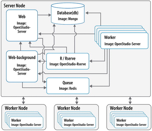
Docker allows the configuration of central processing unit (CPU) resources for each container by defining the number of CPUs that a container is allowed to use, called ‘reservations.’ The ‘web’ service is the orchestrator of the cluster and has CPU reservations that scale with the size of the cluster (i.e. the number of workers) in order to effectively manage the communication with the other services. It also has ports open outside the swarm for API communication to accept new analyses and enable results handling. The ‘web-background’ service utilizes a single CPU and exists to manage the submitted analyses and monitor their state. The database service also scales CPU reservations according to the size of the cluster, while the queue only uses 1 CPU. Because the parallelization scheme of OSAF is to simultaneously batch as many simulations at the same time as possible (as compared to running each building energy model in a parallel or threaded environment), each worker service is reserved 1 CPU and typically exists on a separate computer than the server node, although any unreserved CPUs on the server node will have workers assigned to them.

The scalability of OSAF comes from the worker service, which is responsible for executing a specified BEM workflow and sending results back to the server node. Each worker is responsible for examining the queue for simulations that need to be run, taking a simulation from the queue and running the specified BEM workflow, and repeating that process until the queue is empty. The number of worker services is limited only by the number of CPUs the user has available, both locally and distributed across other computing instances. The Docker Swarm cluster is configured through a ‘docker-compose.yml’ file, which defines the connections and dependencies of the complete software stack. Deployment constraints and CPU resource reservations can also be defined for each service in the cluster. The configuration file for OSAF is located on the GitHub site (Long, Ball, and Fleming 2013).

The containerization of all the services allows for three different scales of deployment for the practitioner. As depicted in Figure 3, these containers can be deployed to a laptop, run on local server hardware, or take advantage of cloud computing resources such as Amazon Web Services. Each of these deployment paths uses the same problem formulation, an analysis description in JSON format (called the OSA [OpenStudio Analysis]), and the Workflow Gem to run simulations. Each path can also create results in a variety of formats, which can be consumed by simple visualization programmes or complicated business intelligence platforms containing machine learning and artificial intelligence algorithms.

Figure 3. Deployment options of OSAF (laptop vs. local vs. cloud). Note that AWS stands for Amazon Web Services. Marjorie Schott, National Renewable Energy Laboratory.

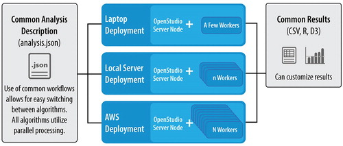
For deployment using Amazon Web Services, practitioners can request 1 server instance, typically a computer with large storage (e.g. 400–1,800 GB) and many CPUs (e.g. 16–72). Practitioners then request ‘n’ number of worker instances (typically a computer with the most CPUs available), each with ‘N’ number of CPUs, resulting in the ability to run n*N number of simulations simultaneously just on the workers alone. Worker services can also be started on the server instance, provided there are enough free CPU resources available. The scale of simulations enabled by OSAF ranges from a simple 2-datapoint comparison to a large study of more than 500,000 datapoints.²

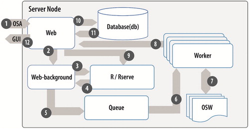
The OSAF simulation process is depicted in Figure 4, which outlines the path of a submitted analysis description file (OSA) through the Docker Swarm architecture (illustrated in Figure 2). The process is enumerated and consists of 12 steps:

1. OSA JSON submitted to the server through the API

2. Problem definition sent to web-background to keep the long running analysis in state

3. Problem definition sent to the R algorithm

4. R algorithm determines variables to run and posts to web-background to create a datapoint JSON for each datapoint

5. Datapoint JSON created from the variable values and queued

6. Worker gets datapoint JSON from the queue and creates a measure-based OpenStudio Workflow file called an OSW

7. OSW is run on the worker and generates results, including objective functions if specified

8. Results and objective functions sent to web (through an HTTP POST request method) over the Docker Swarm network

9. Objective functions sent to the algorithm for possible iteration back to step 4

10. JSON results posted to the database

11. Database results made available to the web front-end

12. Front-end graphical user interface and results API have access to results through the web service.

Figure 4. The OpenStudio Analysis (OSA) simulation process in OSAF (note that GUI stands for graphical user interface and OSW stands for OpenStudio Workflow). Marjorie Schott, National Renewable Energy Laboratory.

3.3. Algorithms compatible with common BEM workflows

As mentioned in Section 2.2, initial attempts to integrate parametric analysis capabilities into OpenStudio began with the integration of DAKOTA into the OpenStudio SDK (Hale et al. 2012). Although this solution seemed promising because DAKOTA was an existing packaged scientific computing library with desirable classes of algorithms (optimization, sensitivity analysis, and uncertainty quantification), in practice the design had shortcomings. It exacerbated the monolithic architecture of the entire code base, which led to poor scalability, and forced users into a Message Passing Interface (MPI)-based environment for parallelization, limiting the deployment capabilities and interoperability with other platforms. Furthermore, typical building parametric analyses can be parallelized in such a way that there is little to no communication needed between building simulation runs. This type of problem is called ‘embarrassingly parallel’ (Herlihy and Shavit 2012). Thus, the MPI-based communication protocol only added unnecessary constraints and complexity to the design.

The current algorithmic framework is designed around the R programming language (R Core Team 2017). R is an open-source, crowd-sourced project with more than 11,000 available user packages.³ It supports parallelization protocols, from individual multicore CPUs, to networked workstations communicating through sockets, and MPI-based clusters. OSAF contains a mix of as-is R packages and several others that are modified to use the socket parallelization scheme available in the Parallel R package (formerly the Snow R Package; see Tierney, Rossini, and Li 2009). All these algorithms are open source, and additional algorithms can be added by making a request or by the users themselves making code changes and submitting a pull request to the OSAF GitHub repository (Long, Ball, and Fleming 2013).

The philosophy of being algorithmically open and inclusive, as well as the open-sourced nature of the licensing framework adopted by all OpenStudio code, is intended to help advance the capabilities of the BEM community and promote private sector adoption of BEM in general. In addition, the framework architecture aims to enable easy comparison and switching between various algorithms to drive both scientific research and commercial-level applications.

The algorithms available in OSAF are detailed in the following three subsections.

3.3.1. Sensitivity analysis and design of Experiment methods

Sensitivity analysis algorithms are used to determine which inputs have the most influence on the outputs and/or determine the range in the output variables given a bounded domain for the inputs. Also, response surface approximations or regression models can be constructed from these methods to create fast-running reduced-order or meta-models when a base building model is too expensive to compute. OSAF algorithms of this type include:

• Full Factorial Design or Design of Experiments

• Morris Screening Method (Campolongo, Cariboni, and Saltelli 2007; Pujol 2009)

• Latin Hypercube Sampling (Stein 1987)

• Monte Carlo Estimation of Sobol Indices (including the methods: Sobol, Sobol-Saltelli, Sobol-Mauntz, Sobol-Jansen, Sobol-Mara, and Sobol-Martinez; see Saltelli 2002; Campolongo, Cariboni, and Saltelli 2007)

• Extended Fourier Amplitude Sensitivity Test (e-FAST99; see Saltelli, Tarantola, and Chan 1999).

3.3.2. Sampling-Based uncertainty quantification

Sampling-based uncertainty quantification algorithms are used where a set of input variable probability distributions are sampled repeatedly, and the selected values are propagated through the simulation model to obtain distributions on the output variables of interest. This can be used to determine the probability of achieving a certain output given defined uncertainty in the inputs. The OSAF algorithm of this type is:

• Latin Hypercube Sampling (Stein 1987).

3.3.3. Optimization and calibration

Optimization and calibration algorithms are used to find the set of inputs that minimize an objective function (such as heating or cooling energy) for an optimal design problem, or the error between simulated and measured energy end uses (such as electric or gas consumption) for a calibration problem. These algorithms can be characterized as single-objective when the objective function is a scalar value and returns a single ‘best’ answer or multi-objective when the objective function is vector-valued and returns a ‘family of best’ answers, typically referred to as Pareto-optimal solutions. Furthermore, because these are all iterative methods, the algorithms can be characterized by how they determine their successive iterations.

The three main categories used in OSAF are: (1) genetic or evolutionary methods, which use heuristics inspired by natural selection to choose the next population of ‘best’ parameters; (2) gradient-based methods where various iterative search directions are chosen based on computing the gradient of the objective function at certain points; and (3) hybrid methods that are a combination of the previous two. Specific OSAF examples are:

• Multi-Objective

  • o Nondominated Sorting Genetic Algorithm 2 (NSGA2; see Deb et al. 2002)

  • o Strength Pareto Evolutionary Algorithm 2 (SPEA2; see Zitzler, Laumanns, and Thiele 2001)

• Single-Objective

  • o R version of GENetic Optimization Using Derivatives (RGenoud; see Mebane and Sekhon 2011)

  • o Particle Swarm Optimization (PSO; see Clerc 2012)

  • o Gradient Search (Optim; see Byrd et al. 1995)

  • o Optimization Using Genetic Algorithms (GA; see Scrucca 2013)

  • o Islands Genetic Algorithms (GAIsl; see Scrucca 2017).

3.4. Common analysis workflow to enable algorithm switching

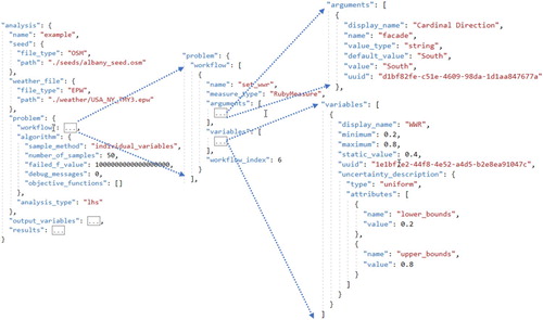
OSAF was developed with the intention of putting advanced energy modelling capabilities in the hands of industry practitioners. To do this, OSAF uses analysis workflows that are shareable, transportable, and reproducible by using a standardized OSA problem definition JSON file, as depicted in Figure 5, and supporting files that can be easily compressed and used on different computing environments. The OSA contains information on the algorithm and its parameters, variables with their uncertainty descriptions (e.g. the minimum and maximum allowed values, normally or uniformly distributed), output variables, and objective functions.

Figure 5. Example of an OpenStudio Analysis (OSA) problem formulation JSON.

In these workflows, individual models are no longer the basis from which the analysis is derived. Instead, the paradigm involves a ‘seed’, which is the baseline model around which the analysis is built, and a chain of scripts, which are run by the Workflow Gem and are used to programmatically implement changes to the baseline model. The scripts, called Measures (Roth, Goldwasser, and Parker 2016; Brackney et al. 2018; Roth et al. 2018), can be generic and reusable across different models and analyses. The chain of scripts and their arguments, as well as the definition of the variables, is described in the ‘workflow’ section of the OSA.

The Measure-based workflow can be described abstractly as a black box mathematical function (1) $y=F(x)$(1) where x is a vector of independent variables or inputs, y is a vector of output variables, and the function F is the application of Measures on the seed model followed by the simulation of the building energy model and any reporting Measures that are part of the workflow and used to compute the output variables. Formulating the problem in this way enables the application and switching between the algorithms described in section 3.3 that operate on the entire BEM based workflow, since the algorithms are designed to operate on processes which can be defined by equation (1). In this context, an independent variable x is simply a Measure input argument that is no longer fixed to a specific value, but one that has an allowed range of values and an uncertainty distribution type. To compute the outputs y, the selected algorithm creates a set of specific x variable values (based on the problem type and variable uncertainty descriptions) along with the information in the workflow section, and eventually gets transformed to a set of specific OSWs, which are then simulated.

The baseline model changes can be varied manually by the user or automatically by an algorithm. Although manually configured analyses are limited by nature in the number of design alternatives they contain, algorithmic analyses can have a much larger number of design alternatives. The use of the same simulation workflow is key to enabling different algorithmic types of analyses (i.e. change from full factorial to sensitivity analysis to uncertainty quantification to optimization to calibration).

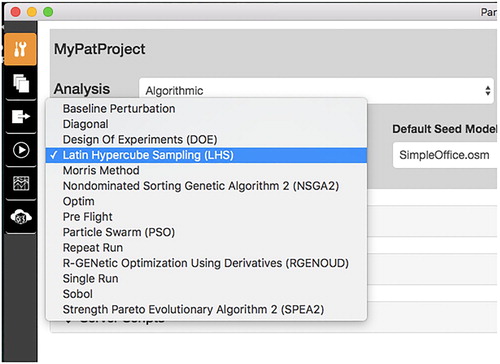
As an example, consider a Measure that changes the window-to-wall ratio in an EnergyPlus model and has two arguments: (1) the window-to-wall ratio (WWR) and (2) the sill height of the base of the window. To change the WWR from a static argument to a variable, the graphical user interface of the Parametric Analysis Tool version 2.0 (OpenStudio Development Team 2016) can be used to easily toggle the variable setting from ‘argument’ to ‘continuous’ and define a minimum and maximum value, as depicted in Figure 6. To implement the change, the Parametric Analysis Tool would then add the WWR argument and its attributes to the ‘variables’ section of the OSA for the user, as depicted on the lower right side of Figure 5. To switch to a different algorithm, users simply change the algorithm section of the OSA, adjust its related parameters to the new algorithm, and run the analysis on OSAF, all while using the same workflow definition. These changes to the OSA can be done manually but using a graphical user interface such as the Parametric Analysis Tool to make the changes, as depicted in Figure 7, can be more efficient and reduces the chances for user error.

Figure 6. Example of defining a Measure variable in the Parametric Analysis Tool graphical user interface.

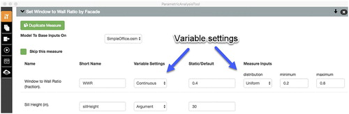
Figure 7. Example of changing algorithm type in the Parametric Analysis Tool graphical user interface.

Community-accepted Measures used in the workflow use the same abstracted methods to make changes to the building energy model (e.g. change window-to-wall ratio, change HVAC system type), which helps further reduce the possible uncertainty introduced by having a human in the modelling loop. Codes and standards routines used at the Measure level ensure consistency and repeatability in the final product – an energy model – which is typically used to calculate energy savings. For example, Natural Resources Canada researchers have developed Measures that support the analysis and development of Canada's National Energy Code for Buildings (Roth 2016). The reproducibility of results when sharing a project among colleagues or clients is also ensured by OSAF, because the same Measures, weather files, seed models, algorithm details, and sequence of operation are incorporated into the project OSA and compressed ZIP file.

3.5. Analyzing BEM results

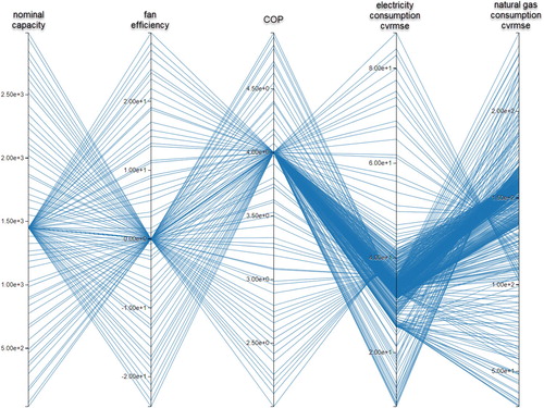
To facilitate quick analysis of BEM results, OSAF has analysis-level visualizations in its web interface for data that persist in the database service of OSAF. Once an analysis is complete, outputs can be sorted and explored via a parallel coordinate plot, as depicted in Figure 8. This interface is interactive: outputs can be turned on or off for plotting, and individual datapoints can be isolated by selecting a range on one of the plot's axes. For example, the plot can be modified to only show those simulations where variable X is within a certain range. The datapoints that satisfy this criterion can then be downloaded and inspected for further analysis.

Figure 8. Example of an Interactive Parallel Coordinate Plot.

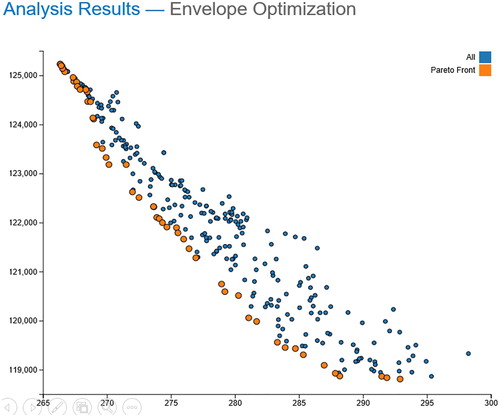
Other plots available include a scatter plot of all the variables in matrix format and an interactive XY plot that allows users to plot one variable against another, including both inputs and outputs. This tool is useful when looking for trends between certain variables. The Pareto front can also be calculated and plotted on the same graph, which is useful for multi-objective optimization problems. Figure 9 depicts an optimization analysis minimizing both energy and envelope costs.

Figure 9. Interactive XY plot with Pareto frontier of annual total energy (gigajoules) vs. envelope cost (dollars).

These types of plots are most useful for small- to medium-scale analyses. The standard OSAF configuration stores all the data in the server node as well as the detailed results from the individual model runs as a compressed ZIP file. This design ensures that the laptop deployment has the same results analysis capability as the cloud-based deployment, and that results can be transferred from the cloud to the local laptop to preserve the model runs after the cloud instances are terminated. Although this works well for smaller problem sets, this approach does not scale well to large-scale analyses, where transferring all the model files back to the server and constantly updating of database information can overload the web service. For large-scale analyses, the data should be transferred to an appropriate external database using the API and analyzed offline with tools specifically developed for this scale (e.g. business intelligence tools).

4. Example case studies

4.1. Calibration

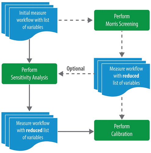
A challenging use case for simulation frameworks is the calibration of building energy models. Calibration can be a large-scale application depending on how many simulations are eventually run by the underlying algorithms. Also, due to the long simulation time of detailed models – ‘long’ meaning the characteristic time is on the order of minutes – parallelization is crucial. Various approaches attempting to solve this challenge have been published. For example, the Python inspyred package, which provides several genetic algorithms, has been used for model calibration (Hong et al. 2017); however, variable selection was limited to what could be substituted in the EnergyPlus input file directly, the algorithm was run manually, and discussion of parallelization on multiple computers (a non-trivial task for most practitioners) was lacking. The authors also relied on previously published sensitivity studies of other building models due to the difficulty in switching between sensitivity-based algorithms and optimization algorithms in the same computing platform and modelling workflow. Algorithm switching is important for calibration because an initial sensitivity study or Morris screening method helps reduce the computational burden by removing inconsequential variables from the parameter space (Reddy, Maor, and Panjapornpon 2007). OSAF addresses this functionality, as depicted in Figure 10, by providing an easy way to change algorithms and reduce variables, simply by editing the OSA JSON.

Figure 10. Algorithm switching for calibration problems. After performing a sensitivity analysis, a Morris screening, or both, inconsequential variables are removed, and algorithms are changed to optimization simply by changing the OSA JSON.

Lara et al. (2017) compared a full-factorial brute force approach to calibration with an evolutionary optimization method using jEPlus via a cloud service. jEPlus (see jEPlus + EA 2011) has similar capabilities to OSAF; however, algorithms are limited to only Latin hypercube and Sobol sampling and NSGA2 for optimization. The model used in Lara et al. was originally created using OpenStudio, but the use of jEPlus forces practitioners to leave the OpenStudio ecosystem and limits model modifications to text substitution schemes on the EnergyPlus input file. OSAF, on the other hand, leverages the Measures and the more powerful methods of the OpenStudio SDK (Roth, Goldwasser, and Parker 2016).

The computational cost of automated calibration has slowed the adoption of these techniques (Hong, Langevin, and Sun 2018) and often forces users to replace detailed models with meta-models. OSAF addresses this issue by providing easy access to cloud computing, which enables direct use of detailed models instead of meta-models in an automated framework. One example is Goldwasser et al. (2018), who performed a detailed time-series calibration on an OpenStudio model of the Oak Ridge National Laboratory's Flexible Research Platform with extensive submetering for validation. Another example is the work done by Studer et al. (2018), in which the National Renewable Energy Laboratory collaborated with the Naval Surface Warfare Center, the U.S. Department of Transportation's Maritime Administration, and the Massachusetts Maritime Academy to evaluate the efficacy of a modified version of EnergyPlus to model naval vessels. During that project, researchers modified EnergyPlus to characterize a moving water boundary condition. They also created special building constructions and calibrated them against time series data from 235 sensor points to see how accurately they could model the thermal behaviour of the hull of a ship. The computational power afforded by OSAF was crucial in these two applications because meta-models could not be used; the former project relied on a detailed calibrated model for automated fault detection and diagnostic purposes, and the latter was a direct validation of EnergyPlus and the proposed modifications for ship-related applications.

The previous examples used traditional optimization algorithms to perform the calibrations. There is increasing interest in Bayesian calibration approaches because of their ability to incorporate and propagate parameter and modelling uncertainty into the final calibration results (Chong and Menberg 2018). Due to the computationally expensive nature of these approaches, meta-models or surrogates are used in lieu of detailed building energy models in the algorithms. Meta-models in this context can help quantify and characterize the model inadequacy in the more detailed model. To generate the meta-models, Bayesian calibration algorithms typically require a training dataset as an input. OSAF can facilitate this by first leveraging the workflow outlined in Figure 10 to identify and retain only the influential model parameters for calibration in the more detailed building energy model. Next, the Latin hypercube or Sobol sampling methods can be used to generate the training dataset from which the meta-models are created by sampling the appropriate parameters as outlined in Chong and Menberg (2018). Parallelization for this step is natural because the parameter sample is computed in full beforehand.

4.2. Leveraging OSAF's API and results in Third-Party tools

OSAF has helped process large-scale BEM analysis results by exporting results in different data formats and sending data to other storage instances to be persisted and analyzed after the simulation cluster is terminated. This approach has worked well for large-scale stock modelling and is detailed in Wilson and Merket (2018) for the ResStock™ project. This project ran more than 350,000 residential building models using OSAF; each model had approximately 100 building input characteristics and more than 30 output metrics. This effort resulted in about a billion datapoints, requiring the authors to create their own interactive visualization tool using a custom database and web interface.

The Parametric Analysis Tool interface is only one way to use the OSAF. Boxer, Henze, and Hirsch (2017) used OSAF's spreadsheet API (Long and Ball 2016) to access the uncertainty analysis capability of OSAF as a basis for their updated Energy Signal Tool for portfolio-level fault detection. Again, results from OSAF were formatted to be easily incorporated into their tool design and application.

As another example, Goel et al. (2018) used OSAF to manage the large quantity of simulation runs needed to create the latest version of DOE's Building Energy Asset Score tool and to provide the data set for the underlying meta-models using a Random Forest algorithm. The data and meta-models were then used as the backbone of the Building Energy Asset Score tool.

The global architecture firm Perkins + Will developed the cloud-based SPEED energy simulation platform using OSAF to provide analytics and simulation capabilities (Welle 2018). They created their own custom interfaces, geared toward architects on the front end. Their early design tool incorporates daylighting analysis by coupling Radiance and EnergyPlus runs on OSAF, thus enabling detailed BEM in the early building design phase at scale. Simulation results are transferred from OSAF to their own database, which has a custom back end for internal company design discussion and review.

The Vermont Energy Efficiency Corporation uses OSAF as part of its technical resource manual (TRM) development and management services. TRMs describe the savings calculation methodologies for different energy efficiency measures to be used by utilities. To accomplish this, TRMs typically publish tables of ‘partially’ deemed savings values that feed into more complex savings equations. These values require frequent review and updating to account for changes in savings due to improved baselines, to incorporate new energy efficiency measures, and to account for changes in available product efficiencies of existing efficiency measures. TRM savings calculations are often based on a set of regulatory-approved representative prototype energy models. One of the Vermont Energy Efficiency Corporation's goals is to convert prototype models from older (DOE-2) simulation engines into more modern and capable (EnergyPlus) versions. To accomplish this, employees use OSAF to generate sets of perturbed OpenStudio versions of each prototype. A calibration-based OSAF workflow is then used to identify families of prototype models that match (within tolerances) various output data elements from the legacy simulations. This cost-effective process supports the development of recommendations for equivalent models as part of a TRM modernization process. Once equivalent prototype buildings are approved, the company uses OSAF to explore perturbed variants of covered energy conservation measures to each prototype. Savings results are used to update TRM published savings tables.

After a few years of deliberation, in January 2020, the New York State Public Service Commission released an order stating, ‘New York should be working on adopting open source technologies such as the U.S. Department of Energy supported EnergyPlus and OpenStudio’ (see Case 18-M-0084 2020). The order also recommends that utilities serving New York state ratepayers should ‘investigate opportunities for implementing a modern framework of open source standardized simulation-based calculation methods supporting an expanding range of state-of-the-art energy efficiency technologies.’ In support of this, Performance Systems Development is working with the New York State Energy Research and Development Authority to develop an OSAF-based calculator for delivering cloud-based ‘dynamically deemed’ savings calculations supporting the Heat Pump Ready utility pilot programme (Heat Pump Ready Pilot Manual 2019). OSAF was used to generate and manage ∼300,000 simulations representing programme targeted residences, and results from this parametric study were used to set programme incentive levels for the upcoming cloud-based calculator. A web-based interface, underpinned by OSAF, is being developed to be used by participating envelope improvement and heat pump installation contractors currently participating in the Home Performance with ENERGY STAR® Program. This online calculator tool combines standardized data collection using Home Performance XML and uses OSAF to manage the generation of both customer-facing and utility-commission-approved estimates of energy savings in a secure environment in near real time (Balbach and Thomas 2019).

5. Conclusions and future directions

The OSAF was developed to manage large-scale BEM analyses. Its capabilities include a common workflow that facilitates integration of BEM into the building design process and easy switching between algorithm and problem types. In addition, it enables analysis of results at a variety of scales, on several different computing platforms available to practitioners, using multiple methods. It is designed to be open source, inspectable, easily configurable, scalable, and accommodating to cross-domain solutions through a clearly defined API upon which other applications – both commercial and private – have been built, as shown in by several real world case study examples.

The current and planned future improvements to OSAF are aligned with the future perspectives outlined in Hong, Langevin, and Sun (2018), including:

1. Developing a non-OpenStudio-based workflow, based on PyFMI (Andersson, Akesson, and Fuhrer 2016), to merge the simulation of Modelica, functional mock-up units, and co-simulation with EnergyPlus with the parametric capabilities of OSAF;

2. Adding Python capability to complement the already existing R-based algorithms;

3. Further results handling by creating and publishing Jupyter-style Python notebooks (Kluyver et al. 2016) that interface directly with OSAF;

4. Enhancing the storage capabilities and reducing load on the server API by developing an extensible file system storage mount; and

5. Enabling other cloud platforms besides Amazon Web Services (e.g. Google Compute Engine, Microsoft Azure) using Kubernetes and Helm.

Acknowledgments

This work was authored in part by the National Renewable Energy Laboratory, operated by Alliance for Sustainable Energy, LLC, for the U.S. Department of Energy (DOE) under Contract No. DE-AC36-08GO28308. Funding provided by the U.S. Department of Energy Office of Energy Efficiency and Renewable Energy Building Technologies Office. The views expressed herein do not necessarily represent the views of the DOE or the U.S. Government. The U.S. Government retains and the publisher, by accepting the article for publication, acknowledges that the U.S. Government retains a nonexclusive, paid-up, irrevocable, worldwide license to publish or reproduce the published form of this work, or allow others to do so, for U.S. Government purposes.

Disclosure statement

No potential conflict of interest was reported by the author(s).

Additional information

Funding

This work was supported by National Renewable Energy Laboratory: [Grant Number DE-AC36-08GO28308].

Notes

1 In 2003, ‘large-scale’ meant roughly 30,000 EnergyPlus simulations on 2003-era desktop computers. This equated to roughly 10,000 to 30,000 core hours of simulations when modeling larger buildings (Hong, Buhl, and Haves 2008).

2 Running more simulations is possible by chaining multiple analyses together and is an active area of development.

3 http://blog.revolutionanalytics.com/2016/03/16-years-of-r-history.html

References

- Adams, B. M., L. E. Bauman, W. J. Bohnhoff, K. R. Dalbey, M. S. Ebeida, J. P. Eddy, M. S. Eldred, et al. 2009. DAKOTA, A Multilevel Parallel Object-Oriented Framework for Design Optimization, Parameter Estimation, Uncertainty Quantification, and Sensitivity Analysis: Version 5.4 User's Manual. Technical Report. Sandia National Laboratories: Albuquerque, NM. SAND2010-2183.
- Andersson, C., J. Åkesson, and C. Führer. 2016. PyFMI: A Python Package for Simulation of Coupled Dynamic Models with the Functional Mock-up Interface. Technical Report, Centre for Mathematical Sciences, Lund University, Lund, Sweden, Volume 2016, No. 2.
- Attia, S., M. Hamdy, W. O’Brien, and S. Carlucci. 2013. “Assessing Gaps and Needs for Integrating Building Performance Optimization Tools in Net Zero Energy Buildings Design.” Energy and Buildings 60 (5): 110–124.
- Balbach, C., and G. Thomas. 2019. “Data Standards, Energy Efficiency and the Digital Data Economy.” Building Performance Association. Accessed February 16, 2020. https://www.hpxmlonline.com/2019/03/12/data-standards-energy-efficiency-and-the-digital-data-economy/.
- Boxer, E., G. P. Henze, and A. I. Hirsch. 2017. “A Model-Based Decision Support Tool for Building Portfolios Under Uncertainty.” Automation in Construction 78 (2017): 34–50.
- Brackney, L., A. Parker, D. Macumber, and K. Benne. 2018. Building Energy Modeling with OpenStudio. Springer. ISBN 978-3-319-77809-9. doi:10.1007/978-3-319-77809-9.
- Byrd, R. H., P. Lu, J. Nocedal, and C. Zhu. 1995. “A Limited Memory Algorithm for Bound Constrained Optimization.” SIAM Journal on Scientific Computing 16 (5): 1190–1208.
- Campolongo, F., J. Cariboni, and A. Saltelli. 2007. “An Effective Screening Design for Sensitivity Analysis of Large Models.” Environmental Modelling & Software 22 (10): 1509–1518.
- Case 18-M-0084. 2020. “In the Matter of a Comprehensive Energy Efficiency Initiative; Order Authorizing Utility Energy Efficiency and Building Electrification Portfolios Through 2025.” State of New York Public Service Commission. Issued January 16. http://documents.dps.ny.gov/public/Common/ViewDoc.aspx?DocRefId={06B0FDEC-62EC-4A97-A7D7-7082F71B68B8}.
- Chong, A., and K. Menberg. 2018. “Guidelines for the Bayesian Calibration of Building Energy Models.” Energy and Buildings 174 (2018): 527–547.
- Christensen, C., R. Anderson, S. Horowitz, A. Courtney, and J. Spencer. 2006. BEopt™ Software for Building Energy Optimization: Features and Capabilities. Technical Report. National Renewable Energy Laboratory. Golden, CO: NREL. /TP-550-39929.
- Clerc, M. 2012. “Beyond Standard Particle Swarm Optimisation.” Innovations and Developments of Swarm Intelligence Applications. IGI Global.
- Crawley, D., J. W. Hand, M. Kummert, and B. T. Griffith. 2008. “Contrasting the Capabilities of Building Energy Performance Simulation Programs.” Building and Environment 43 (4): 661–673.
- Crawley, D., L. K. Lawrie, F. C. Winkelmann, W. F. Buhl, Y. J. Huang, C. O. Pedersen, R. K. Strand, et al. 2001. “EnergyPlus: Creating a New-Generation Building Energy Simulation Program.” Energy and Buildings 33 (4): 319–331.
- Deb, K., A. Pratap, S. Agarwal, and T. Meyarivan. 2002. “A Fast and Elitist Multiobjective Genetic Algorithm: NSGA-II.” IEEE Transactions on Evolutionary Computation 6 (2): 182–197.
- Eisenhower, B., Z. O'Neill, V. A. Fonoberov, and I. Mezić. 2012. “Uncertainty and Sensitivity Decomposition of Building Energy Models.” Journal of Building Performance Simulation 5 (3): 171–184.
- Ellis, P., P. Torcellini, and D. Crawley. 2008. “Energy Design Plugin: An EnergyPlus Plugin for SketchUp.” IBPSA-USA SimBuild, Berkeley, CA, July 30–August 1. National Renewable Energy Laboratory: NREL/CP-550-43569. https://www.nrel.gov/docs/fy08osti/43569.pdf.
- EnergyPlus Example File Generator. 2013. U.S. Department of Energy, Office of Energy Efficiency and Renewable Energy. Accessed December 14, 2017. https://energy.gov/eere/buildings/downloads/energyplus-file-generator.
- Gestwick, M. J., and J. A. Love. 2014. “Trial Application of ASHRAE 1051-RP: Calibration Method for Building Energy Simulation.” Journal of Building Performance Simulation 7 (5): 346–359.
- Giarratano, J. C. 2002. “CLIPS: User’s Guide (version 6.24).” Accessed February 16, 2020. http://clipsrules.sourceforge.net/documentation/v624/ug.htm.
- Goel, S., H. Horsey, N. Wang, J. Gonzalez, N. Long, and K. Fleming. 2018. “Streamlining Building Energy Efficiency Assessment Through Integration of Uncertainty Analysis and Full Scale Energy Simulations.” Energy and Buildings 176: 45–57.
- Goldwasser, D., B. L. Ball, A. Farthing, S. Frank, and P. Im. 2018. “Advances in Calibration of Building Energy Models to Time Series Data.” Building Performance Analysis Conference and SimBuild, Chicago, IL, September 26-28.
- Griffith, B., N. Long, P. Torcellini, R. Judkoff, D. Crawley, and J. Ryan. 2008. Methodology for Modeling Building Energy Performance Across the Commercial Sector. National Renewable Energy Laboratory: Golden, CO. NREL/TP-550-41956. https://www.nrel.gov/docs/fy08osti/41956.pdf.
- Griffith, B., P. Torcellini, N. Long, D. Crawley, and J. Ryan. 2006. Assessment of the Technical Potential for Achieving Zero-Energy Commercial Buildings. National Renewable Energy Laboratory: Golden, CO. NREL/TP-550-41957. https://www.nrel.gov/docs/fy08osti/41957.pdf.
- Guglielmetti, R., D. Macumber, and N. Long. 2011. “OpenStudio: An Open Source Integrated Analysis Platform.” Building Simulation, Sydney, Australia, November 14-16. https://www.nrel.gov/docs/fy12osti/51836.pdf.
- Hale, E., D. Macumber, E. Weaver, and D. Shekhar. 2012. “A Flexible Framework for Building Energy Analysis.” ACEEE Summer Study on Energy Efficiency in Buildings, Pacific Grove, CA, August 12-17.
- Heat Pump Ready Pilot Manual. 2019. New York State Energy Research and Development Authority. Accessed February 12, 2020. http://hpwescontractorsupport.com/wp-content/uploads/2019/09/Pilot_Manual_HPR.pdf.
- Herlihy, M., and N. Shavit. 2012. The Art of Multiprocessor Programming, Revised Reprint, 14. San Francisco, CA: Elsevier.
- Hong, T., F. Buhl, and P. Haves. 2008. EnergyPlus Run Time Analysis. Technical Report. Lawrence Berkeley National Laboratory: Berkeley, CA. LBNL-1311E. https://www.osti.gov/biblio/951766.
- Hong, T., J. Kim, J. Jeong, M. Lee, and C. Ji. 2017. “Automatic Calibration Model of a Building Energy Simulation Using Optimization Algorithm.” Energy Procedia 105 (2017): 3698–3704.
- Hong, T., J. Langevin, and K. Sun. 2018. “Building Simulation: Ten Challenges.” Building Simulation 11 (5): 871–898.
- IBPSA. 2019. “Software Listing.” Accessed December 14, 2017. https://www.buildingenergysoftwaretools.com/software-listing.
- Jabi, W. 2016. “Linking Design and Simulation Using Non-Manifold Topology.” Architectural Science Review 59 (4): 323–334.
- jEPlus+EA. 2011. “jEPlus+EA Users Guide (v1.4).” Accessed December 9, 2017. http://www.jeplus.org/wiki/doku.php?id=docs:jeplus_ea:start.
- Kluyver, T., B. Ragan-Kelley, F. Pérez, B. Granger, M. Bussonnier, J. Frederic, K. Kelley, et al. 2016. “Jupyter Notebooks—A Publishing Format for Reproducible Computational Workflows.” Positioning and Power in Academic Publishing: Players, Agents and Agendas. IOS Press. https://eprints.soton.ac.uk/403913/.
- L3 Harris Geospatial. 2020. “Interactive Data Language (IDL).” Accessed February 12, 2020. https://www.harrisgeospatial.com/Software-Technology/IDL.
- Lara, R. A., E. Naboni, G. Pernigotto, F. Cappelletti, Y. Zhang, F. Barzon, A. Gasparella, et al. 2017. “Optimization Tools for Building Energy Model Calibration.” Energy Procedia 111 (2017): 1060–1069.
- Long, N., and B. L. Ball. 2016. OpenStudio Analysis Spreadsheet (version 0.4.3). https://github.com/NREL/OpenStudio-analysis-spreadsheet.
- Long, N., B. L. Ball, and K. Fleming. 2013. OpenStudio Server (version 1.0). https://github.com/NREL/OpenStudio-server.
- Long, N., B. L. Ball, K. Fleming, and D. Macumber. 2014. “Scaling Building Energy Modeling Horizontally in the Cloud with OpenStudio.” ASHRAE/IBPSA-USA Building Simulation Conference, Atlanta, GA, September 10-12. National Renewable Energy Laboratory: NREL/CP-5500-62199. https://www.osti.gov/biblio/1226251.
- Long, N., S. Goel, and H. Horsey. 2015. “U.S. Department of Energy’s Building Energy Asset Score Sensitivity and Scale Implementation.” Proceedings of the 14th Conference of International Building Performance Simulation Association, India, December 7-9. http://www.ibpsa.org/proceedings/BS2015/p2712.pdf.
- Long, N., A. Hirsch, C. Lobato, and D. Macumber. 2010. “Commercial Building Design Pathways Using Optimization Analysis.” ACEEE Summer Study on Energy Efficiency in Buildings, Pacific Grove, CA, August 15-20. NREL/CP-550-48264. https://www.nrel.gov/docs/fy10osti/48264.pdf.
- Mebane Jr, W. R., and J. S. Sekhon. 2011. “Genetic Optimization Using Derivatives: The Rgenoud Package for R.” Journal of Statistical Software 42 (11): 1–26.
- Merkel, D. 2014. “Docker: Lightweight Linux Containers for Consistent Development and Deployment.” Linux Journal 239 (2). https://dl.acm.org/doi/10.5555/2600239.2600241.
- Nguyen, A., and S. Reiter. 2015. “A Performance Comparison of Sensitivity Analysis Methods for Building Energy Models.” Building Simulation 8 (6): 651–664.
- Nguyen, A., S. Reiter, and P. Rigo. 2014. “A Review on Simulation-Based Optimization Methods Applied to Building Performance Analysis.” Applied Energy 113 (2014): 1043–1058.
- OpenStudio Development Team. 2014. OpenStudio Workflow Gem. https://github.com/NREL/OpenStudio-workflow-gem.
- OpenStudio Development Team. 2016. Parametric Analysis Tool (version 2.0). Accessed February 12, 2020. http://nrel.github.io/OpenStudio-user-documentation/reference/parametric_analysis_tool_2/.
- OpenStudio Development Team. 2017. OpenStudio (version 2.8.0). https://www.openstudio.net/.
- OpenStudio Development Team. 2019. OpenStudio SDK. https://github.com/NREL/OpenStudio.
- OpenStudio Development Team. 2020. OpenStudio Docker Containers. https://hub.docker.com/u/nrel.
- Pujol, G. 2009. “Simplex-Based Screening Designs for Estimating Metamodels.” Reliability Engineering & System Safety 94 (7): 1156–1160.
- R Core Team. 2017. “The R Project for Statistical Computing.” The R Foundation. Vienna, Austria. https://www.r-project.org/.
- Reddy, A. T., I. Maor, and C. Panjapornpon. 2007. “Calibrating Detailed Building Energy Simulation Programs with Measured Data—Part I: General Methodology (RP-1051).” HVAC&R Research 13 (2): 221–241.
- Roth, A. 2016. “New OpenStudio-Standards Gem Delivers One Two Punch.” U.S. Department of Energy. Accessed December 14, 2017. https://www.energy.gov/eere/buildings/articles/new-openstudio-standards-gem-delivers-one-two-punch.
- Roth, A. 2017. “OpenStudio Comes Full Polygon.” U.S. Department of Energy. Accessed December 14, 2017. https://www.energy.gov/eere/buildings/articles/openstudio-comes-full-polygon.
- Roth, A., J. Bull, S. Criswell, P. Ellis, J. Glazer, D. Goldwasser, and D. Reddy. 2018. “Scripting Frameworks for Enhancing EnergyPlus Modeling Productivity.” Building Performance Analysis Conference and SimBuild, Chicago IL, September 26-28.
- Roth, A., D. Goldwasser, and A. Parker. 2016. “There’s a Measure for That!” Energy and Buildings 117 (2016): 321–331.
- Saltelli, A. 2002. “Making Best Use of Model Evaluations to Compute Sensitivity Indices.” Computer Physics Communications 145 (2): 280–297.
- Saltelli, A., S. Tarantola, and K. P.-S. Chan. 1999. “A Quantitative Model-Independent Method for Global Sensitivity Analysis of Model Output.” Technometrics: A Journal of Statistics for the Physical, Chemical, and Engineering Sciences 41 (1): 39–56.
- Scrucca, L. 2013. “GA: A Package for Genetic Algorithms in R.” Journal of Statistical Software 53 (4): 1–37. https://www.jstatsoft.org/article/view/v053i04/v53i04.pdf.
- Scrucca, L. 2017. “On Some Extensions to GA Package: Hybrid Optimisation, Parallelisation and Islands Evolution.” The R Journal 9 (1): 187–206.
- SQLite (version 3.7.10). 2012. https://www.sqlite.org/index.html.
- Stein, M. 1987. “Large Sample Properties of Simulations Using Latin Hypercube Sampling.” Technometrics: A Journal of Statistics for the Physical, Chemical, and Engineering Sciences 29 (2): 143–151.
- Studer, D., J. Barkyoumb, E. Lee, B. L. Ball, S. Frank, E. Holland, J. Green, W. Robinson, J. Brown, and J. Golda. 2018. “Leveraging Shore-Side, Building Energy Simulation Tools for Use in the Shipboard Environment.” Naval Engineers Journal 130 (2): 129–140.
- Tian, W. 2013. “A Review of Sensitivity Analysis Methods in Building Energy Analysis.” Renewable and Sustainable Energy Reviews 20: 411–419.
- Tian, W., and P. de Wilde. 2011. “Uncertainty and Sensitivity Analysis of Building Performance Using Probabilistic Climate Projections: A UK Case Study.” Automation in Construction 20 (8): 1096–1109.
- Tierney, L., A. J. Rossini, and N. Li. 2009. “Snow: A Parallel Computing Framework for the R System.” International Journal of Parallel Programming 37 (1): 78–90.
- Wang, N., S. Goel, A. Makhmalbaf, and N. Long. 2018. “Development of Building Energy Asset Rating Using Stock Modelling in the USA.” Journal of Building Performance Simulation 11 (1): 4–18.
- Welle, B. 2018. Perkins+Will. Accessed May 2019. https://speedwiki.io/project/.
- Wetter, M. 2001. “GenOpt – A Generic Optimization Program.” Seventh International IBPSA Conference, Rio de Janeiro, Brazil, August 13-15. https://simulationresearch.lbl.gov/wetter/download/IBPSA-2001.pdf.
- Wilson, E., and N. Merket. 2018. “An Interactive Visualization Tool for large-Scale Building Stock Modelling.” Building Performance Analysis Conference and SimBuild, Chicago IL, September 26-28.
- Winkelmann, F., B. Birdsall, W. Buhl, K. Ellington, and A. Erdem. 1993. “DOE-2 Supplement: Version 2.1E.” LBL-34947. Lawrence Berkeley Laboratory, Berkeley, CA. https://doi.org/10.2172/10147851.
- Zitzler, E., M. Laumanns, and L. Thiele. 2001. SPEA2: Improving the Performance of the Strength Pareto Evolutionary Algorithm. Technical Report 103. Computer Engineering and Communication Networks Lab (TIK), Swiss Federal Institute of Technology (ETH) Zurich, Switzerland.