Building energy optimization using surrogate model and active sampling

Abstract

In order to improve the performance of a surrogate model-based optimization method for building optimization problems, a new active sampling strategy employing a committee of surrogate models is developed. This strategy selects new samples that are in the regions of the parameter space where the surrogate model predictions are highly uncertain and have low energy use. Results show that the new sampling strategy improves the performance of surrogate model-based optimization method. A comparison between the surrogate model-based optimization methods and two simulation-based optimization methods shows better performance of surrogate model-based optimization methods than a simulation-based optimization method using the PSO algorithm. However, the simulation-based optimization using Ant Colony Optimization found better results in terms of optimality in later stages of the optimization. However, the proposed method showed a better performance at the early optimization stages, yielding solutions within 1% of the best solution found in the fewest number of simulations.

KEYWORDS:

• Sample selection methods
• artificial neural networks
• building energy efficiency
• surrogate model-based optimization method
• simulation – based optimization method
• meta-heuistic optimization

1. Introduction

Buildings energy use and associated greenhouse gas (GHG) emissions are important global environmental concerns (Ürge-Vorsatz et al. 2015). It is estimated that energy used in buildings contributes 40% of the global final energy demand, and produces almost one-third of global GHG (UNEP, Buildings and Climate Change Summary for Decision-Makers 2009). If no energy saving measures are taken to lower buildings’ energy use, GHG emissions from buildings will be almost double by 2030 (UNEP, Buildings and Climate Change Summary for Decision-Makers 2009).

A common method to improve building energy performance is based on computer simulation and parametric sensitivity analysis techniques, varying one parameter at a time in order to find its optimized value. This technique requires a large number of building simulations for all building parameters, which might be impractical. The main limitation is that this technique neglects the interaction between variables (Pang et al. 2020; Bamdad Masouleh 2018). For example, the optimal size of windows may change with overhang size and building orientation. Thus, parametric sensitivity analysis techniques may miss out on potential energy savings that can result from exploring these interactions (Pang et al. 2020; Bamdad Masouleh 2018).

Building Optimization Problems (BOPs) offer a rigorous framework for exploring new designs or retrofit strategies that manage complex trade-offs in ways that are not possible when using traditional methods. The most commonly used method for solving building optimization problems is simulation-based optimization (also known as software-in-the-loop) (Eisenhower et al. 2012; Nguyen, Reiter, and Rigo 2014), where a building simulation programme (e.g. EnergyPlus) is connected to an optimization algorithm (e.g. particle swarm optimization). In these methods, a building simulation programme plays the role of the objective function (e.g. building energy use) and the decision variables are manipulated by an optimization algorithm to improve the objective function in an iterative process. Computational cost of this method pertains to many parameters such as number of objective functions and variables, and the optimization algorithm. For high dimensional optimization problems, the number of building simulations will increase significantly, which may make this method computationally intractable (Magnier and Haghighat 2010).

Building energy optimization using surrogate models (surrogate model-based optimization) is another method used for BOPs and appears to be promising to find a near-optimal design at a reasonable computational cost (Magnier and Haghighat 2010). A surrogate model (also known as a meta-model), is a mathematical approximation of a system, which is created using data collected by simulations or experiments to describe the behaviour of the original system. There are many methods used to construct a surrogate model of a system, such as Artificial Neural Networks (ANNs), Kriging, and support vector regression (Kecman 2001; Haykin 2009).

The prediction accuracy of a surrogate model depends strongly on the number and informativeness of samples (i.e. the extent that a sample can improve the prediction accuracy of a surrogate model) (Liu, Ong, and Cai 2018). The common sample selection method in BOPs is random sampling, which tends to be computationally inefficient for expensive simulations since it can generate many non-informative samples (e.g. samples with high value of objective function in a minimization problem). Some other space-filling methods (e.g. Latin Hypercube), which aim to select representative samples, have been also applied to improve the performance of a surrogate model for BOPs, however, these methods disregard the informativeness of samples. Nevertheless, it is possible to improve the surrogate model prediction through actively selecting the most informative training samples (McKay, Beckman, and Conover 1979; Westermann and Evins 2019).

Sample selection for BOPs has received some limited attention in literature. Some studies have used the uncertainty estimates provided by Gaussian Process (GP) surrogates to select samples (Tresidder, Alexander, and Forrester 2012; Gengembre et al. 2012; Zhang et al. 2013; Gilan, Goyal, and Dilkina 2016). However, the computational stability and efficiency of GP scale poorly when the number of sample points are large (Østergård, Jensen, and Maagaard 2018), which limits their applicability to complex problems, which may need more training samples to obtain accurate surrogates. On the other hand, ANNs are able to provide accurate building surrogate models at the reasonable computational time (Østergård, Jensen, and Maagaard 2018). However, developing sample selection methods for BOPs using ANN surrogates remains an open question. Moreover, there are no studies benchmarking against ‘passive’ and simulation-based optimization methods to quantify the potential computational improvements using ANN surrogates.

Accordingly, the aim of this research is to develop a novel method based on a new sample selection strategy and a committee of efficient surrogate models to improve the performance of the surrogate model-based optimisation method in terms of solution optimality and computational cost (number of simulations) for BOPs.

In addition, a comparison between surrogate model-based optimisation and simulation-based optimisation with two different optimisation algorithms: PSO algorithm (a widely-used algorithm in BOPs (Nguyen, Reiter, and Rigo 2014)) and ant colony optimisation algorithm for continuous domains (ACOR) (Bamdad Masouleh 2018; Bamdad et al. 2017, 2018),, is made to provide new insights for performance of these two methods in BOPs. In this research, a typical medium-size commercial building in two cities in Australia is considered as the case study.

The remainder of this paper is structured as follows. The next section reviews prior work in building energy optimization, while section 3 details methodology, which comprises the formulation of the optimization problem, surrogate model construction, optimization algorithm and the case study. In section 4, the efficiency of the proposed active sampling method is evaluated by comparing its results to the conventional surrogate model-based optimization method, and to the simulation-based optimization method with two different algorithms. Finally, the last section presents the conclusions and proposed future work.

2. Literature review

This section reviews the existing literature about building energy optimization. Subsequently, studies that applied optimization algorithms in building problems are reviewed in order to identify benchmark methods and algorithms.

Building optimization problems can be categorized into two main groups based on the method applied for optimization: simulation-based optimization and surrogate model-based optimization methods (Eisenhower et al. 2012; Nguyen, Reiter, and Rigo 2014).

Simulation-based optimization (connecting a building simulation programme with a mathematical optimization algorithm) is the most common building optimization problem method and it has been applied in many studies. The extensive body of research in this area has demonstrated that this method can considerably decrease the energy use of buildings (Eisenhower et al. 2012; Nguyen, Reiter, and Rigo 2014; Bamdad et al. 2017; Attia et al. 2013; Bamdad et al. 2019). Performance of this method is heavily dependent on the optimization algorithm. Thus, many studies have been conducted so far with the aim of identifying an efficient algorithm for BOPs (Evins 2013). Wetter and Wright (Wetter and Wright 2004) examined the performance of nine optimization algorithms implemented in GenOpt software, including a gradient-based algorithm, direct search algorithms, a Genetic Algorithm (GA), two versions of particle swarm optimisation, and the Hybrid Particle Swarm Optimisation/Hooke-Jeeves (PSO-HJ) algorithm. Their results showed that the hybrid PSO-HJ algorithm outperforms other algorithms in terms of finding solutions with the largest energy reduction. Kämpf, Wetter, and Robinson (2010) investigated the performance of two algorithms, called the hybrid Covariance Matrix Adaptation Evolution Strategy with the Hybrid Differential Evolution (CMA-ES/HDE) and the hybrid PSO-HJ algorithm in minimization of selected standard benchmark functions and two buildings. It was found that the performance of CMA-ES/HDE was better than the PSO-HJ in problems with less than ten dimensions, while if the number of dimensions exceeded ten, the PSO-HJ performed better. Bamdad et al. (2017) benchmarked the performance of four optimization algorithms: ACOR, particle swarm optimization with inertia weight (PSOIW), Nelder and Mead (NM) and PSO-HJ. The ACOR algorithm showed better performance than other algorithms in terms of convergence speed, consistency, and optimality of final solutions. In another investigation, Bamdad et al. (2018) modified the ant colony algorithm for mixed variables (ACOMV) by adaptively tuning the algorithm’s free parameter to improve the algorithm’s performance. Their results showed that the modified algorithm with the adaptively tuned parameter (ACOMV-M) outperforms both the original ACOMV and PSOIW algorithms. Recently, Waibel et al. (2019) benchmarked sixteen optimization algorithms in fifteen building energy optimization problems. Results showed that PSO along with CMA-ES and GA performs well for BOPs. It was also found that parameters tuned to specific problem dimensions could considerably improve PSO performance.

The second method, surrogate model-based optimization, is based on a mathematical approximation of a system, which is created using data collected by simulations or experiments to describe the behaviour of the original system. Surrogate models have been commonly used in the building science for different purposes (e.g. energy prediction and energy labelling) (Melo et al. 2016). For example, Neto and Fiorelli (2008) compared the results of the neural network method and EnergyPlus with measured energy consumption. It was observed that both models are suitable for energy use forecast in the comparison with actual data, but the neural network model is slightly more accurate than EnergyPlus. Melo et al. (2016) tested six different methods to generate surrogate models for building energy labelling, including multiple linear regression, random forests, multivariate adaptive regression splines, artificial neural networks, the gaussian process and support vector machines. The results showed that the surrogate model generated by ANN has the best performance. It was also found that training time in support vector regression is almost six times more than ANN.

Surrogate models have been widely used in numerous science and engineering optimization problems, many of those having been reviewed in (Jin 2005, 2011). In building optimization problems, many studies have used surrogate models as a solution to reduce computational cost associated with simulation-based optimization method, which may take minutes to hours for each run depending on the complexity of building (Westermann and Evins 2019; Wortmann 2019). According to (Roman et al. 2020), ANN and GP are the most common methods to create surrogate models for BOPs.

Romero et al. (2001) applied a numerical method using a finite volume method to calculate energy equations and used ANNs, GA and simulated annealing to optimize building design parameters. Magnier and Haghighat (2010) used the integration of an ANN and NSGA-II to optimize building energy consumption and thermal comfort. The average relative errors of ANN prediction were obtained around 0.5% and 3.9% for the total energy consumption and predicted mean vote comfort index, respectively. They stated that the optimization process took approximately three weeks, while if the simulation-based optimization method using GA was used, it would require ten years to complete the task. Conraud-Bianchi (2008) used the ANN and GA to optimize building energy use, thermal and visual comfort. Gossard, Lartigue, and Thellier (2013) used the ANN and NSGA-II to optimize the annual energy use and the summer comfort degree index in a building for two French climates. Brownlee and Wright (2015) applied NSGA-II to find a trade-off between construction cost and building operational energy use. To improve the computational cost, a surrogate model based on radial basis function networks was developed to approximate and filter promising solutions. Some infeasible solutions were also retained in the population. Results showed that the proposed method performs better than solely NSGA-II in two out of three optimization problems. Asadi et al. (2014) applied GA and ANN in a building optimization problem with three objective functions: retrofit cost, thermal discomfort hours and energy use. Bamdad et al. (2017) compared the performance of four optimization algorithms: interior point algorithm (IPA), ACOR, PSO, and a hybrid ACOR-IPA. It was found that ACOR outperformed PSO in using the simulation-based optimization method. It was also observed that when the surrogate model-based optimization method is used, there is no significant difference between the hybrid ACOR-IPA and ACOR (Bamdad Masouleh et al. 2017c). Zemella et al. (2011) employs ANNs in a surrogate optimization approach applied to a simple single-room building with 5 parameters. While the authors use the ANN to select new samples, no benchmarking is done and thus the benefit of the proposed approach is unclear. Moreover, the proposed approach relies on discretization of continuous variables and exhaustive enumeration of the search space, which is unlikely to scale well to more realistically sized BOPs.

Kriging surrogate model was compared with GA for optimization of building CO₂ emissions (Tresidder, Alexander, and Forrester 2011). It was found that optimization using surrogate models leads to finding more reliable optimal solutions with fewer sampling points. The Kriging surrogate model also showed better performance than stand-alone GA on multi-objective optimization problems with discrete variables (Tresidder, Alexander, and Forrester 2012). An advantage of Gaussian process regression model, as opposed to ANN, has the ability to estimate the uncertainty on predictions. This feature has been employed in (Tresidder, Alexander, and Forrester 2012; Gengembre et al. 2012; Zhang et al. 2013; Gilan, Goyal, and Dilkina 2016) as a means of sample selection. For example, Gengembre et al. (2012) used an efficient global optimization approach using a Kriging surrogate model and PSO algorithm to optimize the life cycle cost of a single-zone building. The results indicated that the proposed method reduces the computational time of the optimization problem. However, a limitation of GP is that this method becomes inefficient when the number of training samples is large (Østergård, Jensen, and Maagaard 2018). Østergård et al. compared the performance of six meta-modelling approaches, including linear regression, GP, Neural Network (NN), SVR, random forest and multivariate adaptive regression splines, in 13 diverse problems. Results showed that NN is the most suitable method in terms of accuracy for problems with a large number of training samples (Østergård, Jensen, and Maagaard 2018).

In summary, the application of optimization methods in buildings remains an active research area. Moreover, comparative studies in the literature show that ANNs perform well in constructing surrogate models and they have been widely used in both building energy prediction and optimization problems, and thus they are selected in this research to construct the surrogate model. The common sampling approaches to create an ANN-based surrogate model in BOPs are either Latin Hypercube (LH) or random sampling. These methods (and other space-filling methods) distribute samples across the parameter space without regard to their informativeness. Therefore, the first objective of this study is to develop a novel sample selection method to improve the performance of the surrogate model-based optimization method using ANNs.

The literature review also indicated that there are few studies conducted so far to benchmark the performance of surrogate model-based optimization against simulation-based optimization methods to explore their potential for efficiently solving BOPs. Thus, the second objective of this study is to make a comparison between these two methods to provide new insights into their performance in solving BOPs.

Finally, the literature review conducted above showed that a GenOpt optimization tool with PSO algorithm has been widely used and performed well in the simulation-based optimization method for BOPs, and it is thus chosen in this study to do a benchmark study. ACOR is also selected to be employed as an optimization algorithm in both simulation-based optimization and optimization of surrogate models, as this recently showed a high efficiency in BOPs (outperforming PSO in a similar case study).

3. Methodology

3.1. Problem statement

The building optimization problem considered in this research is as follows: (1) $\begin{array}{r}minf(x{)}_{\mathrm{s}\mathrm{u}\mathrm{b}\mathrm{j}\mathrm{e}\mathrm{c}\mathrm{t}\mathrm{t}\mathrm{o}:\mathbf{x}\in \mathbb{X}\subseteq {\mathbb{R}}^n}\end{array}$(1) where $f(\cdot ):\mathbb{X}\to \mathbb{R}$ is the objective function, $\mathbb{X}\subset {\mathbb{R}}^n$ is the feasible space, $\mathbf{x}=\left[{\text{x}}_1,{\text{x}}_2,\dots ,{\text{x}}_n\right]$ is the vector of independent design variables. The feasible design space is stated in terms of lower and upper bounds on parameters: $-\mathrm{\infty }<l_i\le x_i\le u_i<+\mathrm{\infty },i=1,2,\dots ,n$ where ${\ell }_i$ and $u_i$ are the lower bound and the upper bound of the variable $\text{i}$. In this research, all decision variables are normalized between zero and one (i.e. $\ell =0$ and $u=1$).

The objective function, $f(\cdot )$, is the normalized building annual end-use energy consumption $\left(\text{MJ}/{\text{m}}^2\text{ Year}\right)$, which is calculated by EnergyPlus (EnergyPlus Energy Simulation Software 2015) and can be written as follows: (2) $\begin{array}{r}f\left(\mathit{x}\right)=E_c\left(\mathit{x}\right)+E_h\left(\mathit{x}\right)+E_l\left(\mathit{x}\right)+E_f\left(\mathit{x}\right)+E_p\left(\mathit{x}\right)+E_m\left(\mathit{x}\right)\end{array}$(2) where $E_c$is the energy use for space cooling $\left(\text{MJ}/{\text{m}}^2\text{ Year}\right)$, $E_h$ is the energy use for space heating $\left(\text{MJ}/{\text{m}}^2\text{ Year}\right)$. $E_l$ is the energy use of lighting $\left(\text{MJ}/{\text{m}}^2\text{ Year}\right)$., $E_f$ is the energy use of the supply and return fans of HVAC system $\left(\text{MJ}/{\text{m}}^2\text{ Year}\right)$, $E_p$is the energy use of pumps $\left(\text{MJ}/{\text{m}}^2\text{ Year}\right)$, and $E_m$ is the energy use of both cooling tower heat rejection and interior equipment $\left(\text{MJ}/{\text{m}}^2\text{ Year}\right)$.

3.2. Artificial neural networks

Artificial neural networks are selected to construct a surrogate model, as the literature review has found they perform well in both building energy prediction and BOPs. ANNs are computer-learning models, which were inspired by biological neural networks, that mimic the learning process of the human brain (Haykin 2009). The first computational model of neural networks was introduced in (McCulloch and Pitts 1943) and they have been shown to be universal approximators (Hornik, Stinchcombe, and White 1989; Kůrková 1992). In ANNs, the output of a neuron can be calculated as follows: (3) $\begin{array}{r}y=f\left(\sum _{i=1}^n{w}_i{x}_i+b\right)\end{array}$(3) where $x_i$ represents the ith input of the neuron, $w_i$ is the weight associate with ith input and $b$ is the bias. In order to identify the values of weights, the network is trained using historical data, and the optimal value of the weights is found by minimizing the Mean-Squared Error (MSE) output of the network (predicted values) and actual (desired) values.

The Levenberg-Marquardt (LM) algorithm is an efficient optimization algorithm that has been widely used for training ANN weights (Kecman 2001; Ascione et al. 2017; Haykin 1998) and is recommended as a first-choice algorithm for supervised learning problems (Demuth, Beale, and Hagan 2006). This algorithm with Bayesian regularization is used for training the network to avoid overfitting problem (i.e. low training error with poor generalization to new data) (Demuth, Beale, and Hagan 2006).

A key issue affecting the performance of ANNs is the number of neurons in hidden layers. The number of neurons depends strongly on the problem and should be properly selected. Too many neurons in the hidden layers can lead to overfitting. On the other hand, if the number of neurons in the hidden layers is too few, the model fails to capture the trend of the data (under-fitting). Thus, finding a balance between the fitting performance and the generalization performance is essentially a question of determining the number of hidden neurons, which are often determined using cross-validation method (Haykin 2009).

In the cross-validation method, some of the training data is removed from the training set and used to assess the generalization performance of the model (Meckesheimer et al. 2002). For $K$-fold cross-validation, training data are divided into $K$ subsets of (approximately) equal size and then the network is trained $K$ times so that each time, one of the subsets is left out from training data and used as test data, and the remaining (K−1) data sets are used for training the network. The model performance is then expressed as the average prediction (generalization) error over all $K$ test folds. The optimal number of hidden neurons can be found by performing a grid search over the hidden layer sizes, and selecting the number of neurons that result in the lowest average prediction error over the $K$-folds. Thus, the $K$-fold cross-validation process is repeated until the model generalization error stops improving for a specific number of iterations. Finally, the model with the minimum prediction error (i.e. maximum generalization performance) is chosen.

The key parameter in this method is the value of $K$, which should be selected appropriately (Chou and Bui 2014). Although there are no generally accepted mathematical formulae for determining the number of neurons in the hidden layer (Mba, Meukam, and Kemajou 2016), Kohavi (1995) investigated the effect of different values of $K$ on many real-world datasets and their results showed that the cross-validation method with ten folds is suitable for model validation.

3.3. Selection of training samples

For surrogate modelling applications, it is significant to select samples efficiently for training the ANN due to the relatively high computational cost of building simulators. The efficiency of this selection can strongly influence the overall computational cost and the optimality of solutions produced by the surrogate approach.

Commonly, Latin Hypercube (LH) or random sampling are utilized to select samples, and these samples are then evaluated (labelled) by the building simulator to produce training data for the surrogate model. After training, the surrogate is used in an optimization routine. Yet, the random sampling, LH, and other space-filling methods distribute samples across the parameter space without regard for their informativeness. From an optimization perspective, this is not efficient since high accuracy is only required in promising regions of the parameter space (i.e. regions with low energy consumption).

In contrast to these passive approaches, this study aims to provide an active sample selection method that attempts to refine the surrogate model in promising (i.e. low energy) regions of the parameter space. The proposed method utilizes a modified uncertainty sampling (Settles 2012; Krogh and Vedelsby 1995), where the aim is to find informative training samples in regions of the parameter space where the predicted energies are low (around the local minima).

Let ${\mathcal{L}}^{\left(0\right)}=\{\left({\mathit{x}}_n,f\left({\mathit{x}}_n\right)\right){\}}_{n=1}^N$ denote the initial training dataset composed $N$ labelled samples and ${\mathcal{U}}^{\left(0\right)}=\{{\stackrel{\mathbf{ˆ}}{\mathit{x}}}_m{\}}_{m=1}^M$ denote the initial pool of $M$ unlabelled samples where $M\gg N$. In order to generate a set of samples, Latin Hypercube Sampling (LHS) is used to generate both $\mathcal{L}$ and $\mathcal{U}$ to ensure efficient coverage of the entire parameter space (McKay, Beckman, and Conover 1979).

In order to select the most informative unlabelled samples for labelling, a committee consisting of $L$ surrogate models, is built using the initial labelled dataset $\left(\mathcal{L}\right)$ with different weight initializations (so that each ANN may achieve a different local optimum). Each surrogate model predicts the label of every unlabelled sample point in the unlabelled pool of data set $\left(\mathcal{U}\right)$. Let the predicted values by the $\ell$th committee member for ${\hat{x}}_m$ be ${\hat{y}}_m^{\ell }$. Then, the mean and variance of predicted values for ${\hat{x}}_m$ over all $L$ committee members may be calculated as follows: (4) $\begin{array}{rl}{\overline{y}}_m& =\frac{1}{L}\sum _{\ell =1}^L{\hat{y}}_m^{\ell }\end{array}$(4) (5) $\begin{array}{rl}{s}_m^2& =\frac{1}{L-1}\sum _{\ell =1}^L({\hat{y}}_m^{\ell }-{\overline{y}}_m{)}^2\end{array}$(5)

In this method, the variance of samples provides an idea of the level of dizagreement between surrogate models. Samples with higher variance are those that are more uncertain and could add more information to improve the surrogate model prediction accuracy. Thus, unlabelled sample points are then sorted from the highest to the lowest variance and the first $k$ unlabelled samples $\left(k\le M\right)$ with the highest variances are good candidates for new samples to label. However, it is also highly desirable to select samples that have low predicted energy use since these samples are more likely to be near the optimal parameters. Thus, a condition on the objective value of the selected samples is set as well. Let $\overline{\mathit{y}}=\left\{{\overline{y}}_1,{\overline{y}}_2,\dots ,{\overline{y}}_M\right\}$ be the vector of predicted mean value of unlabelled samples. In an effort to select samples to improve the accuracy of the surrogate model in promising regions (regions with low energy), new samples are selected as candidates for labelling: (6) $\begin{array}{r}\hat{\mathcal{U}}=\left\{{\stackrel{\mathbf{ˆ}}{\mathit{x}}}_m|{\overline{y}}_m<\text{Percentile}\left(\overline{\mathit{y}},p\right),m=1,2,\dots ,M\right\}\end{array}$(6) where $\text{Percentile}\left(\overline{\mathit{y}},p\right)$ is a function that returns the pth percentile of unlabelled samples in the pool and decreases at each optimization iteration. The samples to be labelled can then be selected from this set.

3.4. Proposed surrogate model based optimization method

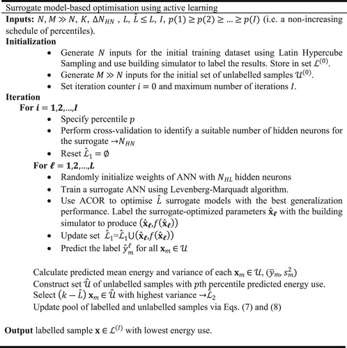
A new surrogate-based optimization method called Surrogate model-based Optimization using Active Sampling (SOAS) is developed in this section (the overall algorithm summarized in Figure 1). In this method, first an initial surrogate model is constructed using the labelled samples $\mathcal{L}$ (initial training dataset) generated by LHS. In the next step, in order to identify the best architecture of the netwo (i.e. number of hidden neurons), $K$-fold cross validation is applied. The network is then trained $L$ times with different random weight initializations to build a committee of networks consisting of $L$ surrogate models. Due to the different initialization of the weights, each of the $L$models will likely have different weights, resulting in a network with different accuracies.

Figure 1. Surrogate model-based optimization using active sampling.

At this point, $\hat{L}\in \left[1,L\right]$. surrogate models are optimized. Two variants of the algorithm are used:

1. $\hat{L}=1$. The best surrogate model (i.e. surrogate model with the best generalization performance) in the committee is used for optimization in each iteration.

2. $\hat{L}=L$. All members of committee are optimized in each iteration.

Since the optimization process does not require any further building simulations (only evaluation of the surrogate model), each optimization is much faster than the EnergyPlus-in-the-loop approach. The ACOR algorithm is used for optimization of surrogate model(s) and $\hat{L}$ optimized solutions are stored in a library for future labelling via building simulation software. In each iteration, the objective function of corresponding optimized solution(s) is calculated by EnergyPlus and compared with its value from previous iterations and then the library is updated with the smaller value. The solution stored in the library represents the best solution found so far.

If the stopping criteria (e.g. maximum number of iterations) are not satisfied, the next step is to add new samples to the labelled set to refine the surrogate models. Consider the current sets of unlabelled and labelled samples ${\mathcal{U}}^{\left(i\right)}$ and ${\mathcal{L}}^{\left(i\right)}$, respectively. For the next iteration, two strategies are used to select $k$ new samples for labelling:

1. Optimized solutions. The $\hat{L}$ optimized solutions obtained by the committee of surrogate model(s) in the current iteration are labelled (evaluated) by the building simulator (e.g. EnergyPlus) and stored into a new set ${\hat{\mathcal{L}}}_1.$ These samples are likely close to local minima and hence they have the potential to improve the model prediction accuracy in promising regions (resulting in local refinement).

2. Samples with high ambiguity and low energy use. The proposed sample selection method stated in section 3.3 is used to generate the set $\mathcal{U}$ from which the remaining $k-\hat{L}$ new samples are selected. The variance and mean of each sample $\mathbf{x}\in \hat{\mathcal{U}}$ are then calculated using Equations (4) and (5). Let ${\hat{\mathcal{U}}}_1\subseteq \hat{\mathcal{U}}$ be the set of $k-\hat{L}$ samples with the largest variance. These samples are then labelled by the building simulator, and stored into a set of newly labelled samples ${\hat{\mathcal{L}}}_2$. The sample pools are then updated for the next iteration as (7) $\begin{array}{rl}{\mathcal{L}}^{\left(i+1\right)}& ={\mathcal{L}}^{\left(i\right)}\cup {\hat{\mathcal{L}}}_1\cup {\hat{\mathcal{L}}}_2\end{array}$(7) (8) $\begin{array}{rl}{\mathcal{U}}^{\left(i+1\right)}& ={\mathcal{U}}^{\left(i\right)}\mathrm{\setminus }{\hat{\mathcal{U}}}_1\end{array}$(8)

The algorithm then proceeds to the next iteration, starting with the grid search and $K$-fold cross validation to find the number of hidden neurons. However, since only a small number of new samples have been added to the training dataset, the optimal number of hidden neurons in the previous iteration should be close to the number from the previous iteration. Thus, the following equation has been introduced to efficiently identify the optimized number of hidden neurons: (9) $\begin{array}{r}{N}_{HN}^{\left(i-1\right)}-\mathrm{\Delta }{N}_{HN}\le N_{HN}^{\left(i\right)}\le N_{HN}^{\left(i-1\right)}+\mathrm{\Delta }{N}_{HN}\end{array}$(9) where $N_{HN}^{\left(i\right)}$ is the best number of hidden neuron identified by $K$-fold cross-validation method at the $i$th iteration and $\mathrm{\Delta }{N}_{HN}$ is the half-width of the grid search interval. Obviously, the lower bound cannot be less than or equal to zero so it is saturated at one. The algorithm then proceeds with training the committee, optimization, and sample selection as above. The overall algorithm is summarized below.

3.5 Optimization algorithm

Ant colony optimization is a metaheuristic algorithm that was inspired by observations of ant behaviour. This optimization algorithm was first designed to address discrete optimization problems and later extended to solve problems with continuous variables (Socha and Dorigo 2008; Dorigo, Maniezzo, and Colorni 1996). This extension, ACOR algorithm, has performed well in solving building energy optimization problems in previous studies (Bamdad et al. 2017; Bamdad et al. 2018; Bamdad Masouleh et al. 2017c).

ACOR operates on a solution archive, which is shown in Figure 2. This archive contains the values of the $N$ decision variables ${\mathit{x}}_{\mathit{j}}=\left[x_j^1,x_j^2,\dots ,x_j^N\right]$ and the associated objective function values $f\left({\mathit{x}}_{\mathit{j}}\right)$. It should be noted that the values of $f\left({\mathit{x}}_{\mathit{j}}\right)$ are calculated by building simulation software. Solutions in the archive are sorted from lowest to highest objective values, i.e. (10) $\begin{array}{r}f\left({\mathit{x}}_1\right)\le f\left({\mathit{x}}_2\right)\le \dots \le f\left({\mathit{x}}_j\right)\le \dots \le f\left({\mathit{x}}_M\right)\end{array}$(10)

Figure 2. Solution archive for ACOR [adapted from (Socha and Dorigo 2008)].

New candidate solutions are generated according to a Gaussian kernel probability density function (PDF) based on the solutions in the archive. For a more detailed description of this algorithm, please refer to (Bamdad et al. 2017, 2018; Bamdad Masouleh et al. 2017c).

3.6. Building simulation

Building Type B is a three-storey office building with heavy-weight concrete construction and a gross floor area of 2003.85 m². The Australian Building Codes Board (ABCB) (2002a, 2002b) has recommended this building to represent the typical medium-size office buildings in Australia. A variable air volume system with water-cooled chiller (COP = 3.57) was modelled for this building with the heating and cooling sizing factors of 1.25. The details of building Type B are given in Figure 3, Tables 1 and 2. The schedules used for occupancy, lighting (limited control), equipment and HVAC working hours were the same as given by the National Australian Built Environment Rating System (NABERS) (2011).

Figure 3. Three-storey building Type B (ABCB) (Board, A.B.C. 2002a; Board, A.B.C. 2002b).

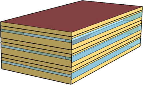
Table 1. Building construction details (Board, A.B.C. 2002a).

Component	Construction Materials	U-Value (W/m^2K)
Wall	200 mm heavy weight concrete R1.5 batts, 10 mm plasterboard (absorption coefficient=0.6)	0.520
Roof	Metal deck, air gap, 150 mm heavy weight concrete, roof space, R2.0 batts, 13 mm acoustic tiles (absorption coefficient=0.6)	0.267
Floors	175 mm concrete, carpet 2.7 cm	1.351
Windows Window to wall ratio	6 mm clear glass 37.5% (E & W faces), 15% (N & S faces)	5.89
Overhang	NA

Table 2: Building geometry details and assumptions used in building simulation (Board, A.B.C. 2002a).

Parameters	Values
Total floor area (m^2)	2004
Geometry (m)	36.5 × 18.3
Number of floors	3
Floor to ceiling height (m)	2.7
Floor to floor height (m)	3.6
Equipment load	15 W/m^2
Lighting load	15 W/m^2
Lifts and auxiliary service equipment	1 W/m^2
Occupancy	0.1 Person/m^2
Temperature set-point	20–24°C
Temperature set-back	28°C (18:00-07:00, business days)
Ventilation requirement	10 (L/s/person)
Infiltration	1 ACH outside HVAC operating hours, no infiltration during HVAC hours

4. Results

Surrogate model-based optimization using random sampling, the proposed SOAS method, and simulation-based optimization method using PSO and ACOR algorithms, are applied to building Type B to minimize the annual energy consumption (Equation (2)) with respect to 15 variables listed in Table 3. Two different Australian climates, Brisbane with warm humid summers and mild winters, and Melbourne with warm summers and cool winters, are considered in this research. The average number of variables in BOPs was selected here (Nguyen, Reiter, and Rigo 2014), and the feasible search intervals were determined according to other similar studies.

Table 3: Optimization variables and their range.

Variables	Description	Initial Value	Variable Range
x1	Roof emissivity	0.7	[0.5–0.9]
x2	Roof solar absorptance	0.7	[0.3–0.85]
x3	Wall insulation (cm)	4.5	[1–10]
x4	Wall solar absorptance	0.7	[0.3–0.9]
x5	North window height (m)	1.35	[0.5–1.5]
x6	South window height (m)	1.35	[0.5–1.5]
x7	East window height (m)	0.54	[0.5–1.5]
x8	West window height (m)	0.54	[0.5–1.5]
x9	North overhang depth (m)	0	[0–1.5]
x10	South overhang depth (m)	0	[0–1.5]
x11	East overhang depth (m)	0	[0–1.5]
x12	West overhang depth (m)	0	[0–1.5]
x13	Heating setpoint (°C)	20	[18–22]
x14	Cooling setpoint (°C)	24	[23–27]
x15	Building orientation (degree)	0	[0–45]

To conduct surrogate model-based optimization, a standard feed-forward multi-layer perceptron ANN with three layers (input, hidden, and output) was used to construct the surrogate model. The sigmoid function was used as the activation function and all input data were normalized between [0, 1]. Latin hypercube sampling method was used to generate a pool of unlabelled samples with $M=15000$ sample points. A MATLAB code was developed to run EnergyPlus automatically and control the whole optimization process, including a network training and optimization algorithm.

The number of neurons in the hidden later was determined via a grid search with $\mathrm{\Delta }{N}_{HN}=5$. The Levenberg–Marquardt back-propagation algorithm with Bayesian regularization was used to train the network. The algorithm parameters were selected based on recommendations in (Demuth, Beale, and Hagan 2006) and listed in Table 4. Once the training process was completed, the ACOR algorithm was applied to optimize the surrogate model(s). The initial surrogate model was built using 50 training samples, which were labelled by EnergyPlus (i.e. EnergyPlus calculates annual end-use energy use, Equation (2), associated with each sample (i.e. each sample includes a set of fifteen variables, the values of which are selected through the Latin Hypercube method)). In each iteration, 50 new samples were added to the training dataset (k=50) and in total 40 iterations were run for the surrogate model-based optimization method (i.e. 2000 building simulations). The committee of surrogate models contains five members $\left(L=5\right)$ with different initializations. To identify the regions with the low energy in the search space, Equation (6) is applied. The values of function $p_i$ are calculated based on Equation (11) where $i$ is the number of iterations, $\mathrm{\Delta }$is the step size and equals to $5\mathrm{\%}$, and $p_0=50\mathrm{\%}.$ The percentile is set to decrease due to the fact that by adding new training samples in each iteration, the prediction accuracy of the surrogate model is gradually improved. Therefore, the surrogate model is more likely to accurately identify the regions with low energy consumption. (11) $\begin{array}{r}{p}_{i+1}=\left\{\begin{array}{cl}{p}_i-\mathrm{\Delta }& \text{if }{p}_i>\mathrm{\Delta }\\ 1\mathrm{\%}& \text{if }{p}_i\le \mathrm{\Delta }\end{array}\right.\end{array}$(11) To conduct the simulation-based optimization, PSOIW (using GenOpt software) and ACOR algorithms were directly connected to EnergyPlus. The algorithms’ parameters were chosen based on the recommendations of previous studies (Kämpf, Wetter, and Robinson 2010; Bui, Soliman, and Abbass 2007) and are listed in Tables 5 and 6. In the PSOIW algorithm, cognitive acceleration and social acceleration are exploration (global search ability) and exploitation (local search ability) operators, respectively. In this algorithm, the inertia weight is used to keep balance between exploration and exploitation. A large value of inertia weight improves exploration while a small value facilitates exploitation (Wetter and Wright 2004).

Table 4: Parameters of Levenberg–Marquardt with Bayesian regularization.

Parameters	Value
Maximum number of epochs to train	2000
Marquardt adjustment parameter	0.005
Decrease factor for mu	0.1
Increase factor for mu	10
Maximum value for mu	1e10
Minimum performance gradient	1e-7

Table 5: Parameters used for ACOR.

Parameters	ACOR
No. of new solutions used in each iteration (ants)	5
$q$ parameter	0.1
Speed of convergence $\left(\xi \right)$	0.85
Archive size	50

Table 6: Parameters used for PSOIW.

Parameters	PSOIW
Topology	Von Neumann
Number of particles	100
Cognitive acceleration	2.05
Social acceleration	2.05
Max velocity gain	0.2
Initial inertia weight	1.0
Final inertia weight	0

Fifteen optimization runs were conducted for each optimization algorithm using High Performance Computing (HPC) cluster, since 2000 building simulations were required for each run. The time required for 2000 building simulations with EnergyPlus 8.1.0 is approximately 25 h.

4.1. Network configuration identification results

A $10$-fold cross validation is selected in this research, which has been recommended by previous studies (Chou and Bui 2014; Kohavi 1995). Mean Squared Error (MSE) is used to evaluate the performance of each network. Before training the network, all data is first normalized to fall between zero and one to ensure numerical stability for the training and optimization. In the network training process, the algorithm terminates when one of the following three criteria are achieved: (1) the number of epochs exceeds 5000; (2) the gradient norm is sufficiently small (1e-10); (3) the mean square error is below 1e-10.

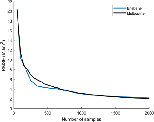
Figure 4 shows the results of $10$-fold cross validation for the ANN for different training samples for Brisbane and Melbourne. As can be seen in the figure, the number of hidden neurons increases with an increase in the number of training samples so that for the network with 2000 training samples, the optimal configurations of the network are 24 and 21 hidden neurons for Melbourne and Brisbane, respectively. The subfigure shows a snapshot of the Root Mean Square Error (RMSE) for different numbers of hidden neurons when there are 500 training samples. As can be seen, the minimum RMSE (0.0045) performance was achieved for a network with 6 hidden neurons for Brisbane. For Melbourne, the optimal configuration was achieved for the network when the number of hidden neurons is 9 and the RMSE error is 0.0053. Figure 5 shows RMSE of $K$-fold cross validation method averaged over 15 runs for both Brisbane and Melbourne. As expected, by adding more samples in the training dataset, the RMSE on the test data decreases.

Figure 4. Results of cross validation method to identify the network architecture.

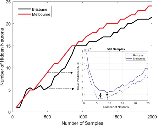
Figure 5. Root mean square error of $K$-fold cross validation method (average of 15 runs)

4.2. Optimization results

Figure 6 shows the median value of results of convergence curve for fifteen runs for Brisbane. This figure compares the results of five different methods, including two simulation-based optimization methods using PSOIW and ACOR algorithms, and three surrogate model-based optimization methods using different sampling strategies: random sampling, SOAS when $\hat{L}=1$ and SOAS when $\hat{L}=5$ (L-SOAS). In this figure, three types of comparisons are worthy of discussion: A first comparison is between different surrogate model-based optimization methods, which shows that the L-SOAS method performs the best, and both active sampling methods outperform random sampling. The second one is between all surrogate model-based optimization methods and the simulation-based optimization method using PSOIW, which shows all surrogate model-based optimizations perform better than PSOIW algorithm. Finally, is the comparison between surrogate models and simulation-based optimization method using ACOR. As can be seen, the surrogate model-based optimization methods are able to find better solutions than simulation-based optimization method using ACOR in the early stages of optimization, but after approximately $1000$ building simulations ACOR is able to achieve superior solutions. The reason is likely due to the approximation error of the surrogate model (Kecman 2001; Ascione et al. 2017; Haykin 1998). As can be seen, after approximately 1000 samples, the surrogate model performance can scarcely improve with increasing number of samples. However, from an energy point of view, these differences are quite small as a percentage of building energy consumption.

Figure 6. Convergence curve of the optimization results for Brisbane (Median value of fifteen runs)

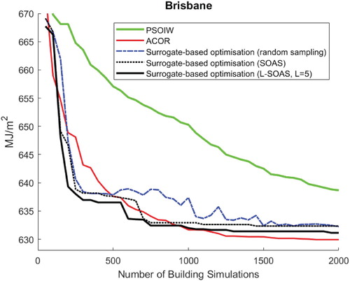
Regarding the optimization time, the network training time of surrogate model-based optimization methods depends on the number of sample points used for training. For example, the time required to find a solution within $1\mathrm{\%}$ of the final optimized solution is approximately 3 min (including time for 10-fold cross validation, network training time and optimization) with 400 training samples. By contrast, ACOR (simulation-based optimization) requires 600 simulations to find the similar solution, which takes 2.5 h longer (i.e. the total optimization time with 600 building simulations is approximately 7.5 h). It should be noted that with more training samples, the training time to create the surrogate model is longer so that with 2000 training samples, the surrogate-based optimization method requires approximately 30 min to find an optimized solution.

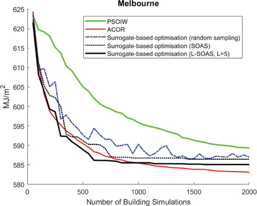
Figure 7 shows the median value of results of convergence curve for fifteen runs for Melbourne. Similar to the results for Brisbane, all surrogate model-based optimization methods outperform PSOIW, and L-SOAS performs the best among surrogate model-based optimization methods. As can be seen, L-SOAS outperforms ACOR at the early stages of optimization, however, ACOR performs better at the later stages of the optimization. Thus, in this example, the surrogate optimization method offers an increase in the early convergence rate, which is further enhanced by the L-SOAS active sampling. However, the advantages of the surrogate approach are lost when the number of labelled samples increases beyond 1000 samples.

Figure 7. Convergence curve of the optimization results for Melbourne (Median value of fifteen runs)

Figures 8 and 9 display the distribution of optimization results based on fifteen different runs for Brisbane and Melbourne respectively. As can be seen at the early stages of optimization, the spread of the optimization results using random sampling is larger than both active sampling methods. However, it improves towards the end of optimization process. With regard to active sampling methods, the variability of L-SOAS improves over the course of optimization and remains relatively small, demonstrating the reliability of this method for BOPs. The ACOR also performs well and the distribution of its optimization results continuously becomes smaller during the optimization process.

Figure 8. Distribution of optimization results based on fifteen different runs for Brisbane

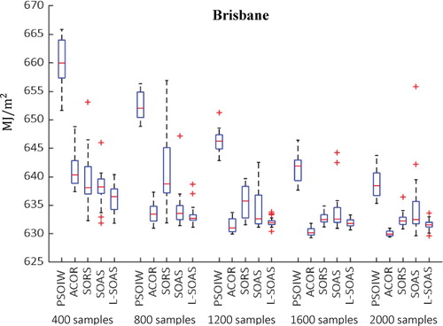
Figure 9. Distribution of optimization results based on fifteen different runs for Melbourne

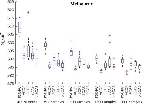
Table 7 shows the best parameter sets among all fifteen runs after 2000 building simulations for each algorithm for Brisbane and Melbourne. It should be noted that in order to compare the optimized values of objective function (i.e. total building energy consumption) all optimized parameters sets (found by either the surrogate or simulation methods) were exported to EnergyPlus for energy evaluation and then reported in this table. As can be seen for both cities, the best solutions (the bold rows in the table) were obtained by ACOR while PSOIW found the worst solution. This table shows that the optimized building orientations are approximately $11$ and $43$ degrees relative to North (clockwise) for Brisbane and Melbourne, respectively. For both cities, the optimized wall has the minimum solar absorptance, and the optimized roof has the maximum emissivity with minimum solar absorptance. For Melbourne, the maximum wall insulation thickness was selected by the optimization algorithm, while the minimum insulation thickness was chosen for Brisbane. This is likely due to Brisbane’s climate, where buildings frequently have a little-to-no heating loads and high internal loads in the buildings during daytime (Cohn, Ghahramani, and Jordan 1996). With regard to window size, the minimum value was selected for all building’ faces, except for the variable $x_{12}$ (west overhang depth) in Brisbane. The optimized value for overhang depends on city and building direction. The maximum and minimum were selected for the cooling and heating set-points for all cities, respectively. This is clearly expected when thermal comfort is not considered in the objective function and only as a constraint on the allowable range of indoor temperature set points.

Table 7: Best parameter sets of optimization results.

	Method	Objective Function (MJ/m^2)	x1	x2	x3	x4	x5	x6	x7	x8	x9	x10	x11	x12	x13	x14	x15
Brisbane	SMRS^a	630.60	0.9	0.3	1	0.3	0.5	0.5	0.5	0.5	0.29	0.25	0.34	0.65	18	27	11.09
	SOAS	630.48	0.9	0.3	1	0.3	0.5	0.5	0.5	0.66	0.35	0.39	0.36	1.50	18	27	8.78
	L-SOAS	630.18	0.9	0.3	1	0.3	0.5	0.5	0.5	0.7	0.33	0.23	0.47	1.50	18	27	10.23
	ACOR	629.62	0.88	0.3	1	0.3	0.5	0.5	0.5	0.72	0.55	0.54	0.54	1.44	18	27	11.11
	PSOIW	635.31	0.72	0.42	1	0.31	0.58	0.57	0.87	0.52	0.63	0.55	0.84	0.39	18	27	24.14
Melbourne	SMRS^a	583.89	0.9	0.3	10	0.3	0.5	0.5	0.5	0.5	0.26	0	0.54	0.89	18	27	0
	SOAS	581.73	0.9	0.3	10	0.3	0.5	0.5	0.5	0.5	0.39	0.43	0.21	0.52	18	27	45
	L-SOAS	581.53	0.9	0.3	10	0.3	0.5	0.5	0.5	0.5	0.38	0.39	0.26	0.54	18	27	40.83
	ACOR	580.51	0.89	0.31	10	0.31	0.5	0.5	0.51	0.51	0.53	0.52	0.24	0.54	18	27	42.76
	PSOIW	585.64	0.79	0.3	8	0.47	0.51	0.5	0.52	0.51	0.37	0.06	0.56	0.82	18	27	9.23

Note: ^aSurrogate with random sampling method (SMRS).

From an energy perspective, the discrepancy between optimized objective functions obtained by ACOR and surrogate model-based optimization using active learning methods may be considered small (in the order of around $0.1\mathrm{\%}$). Despite these small differences, different sets of parameters have been obtained, which shows that the building objective function is very multi-modal.

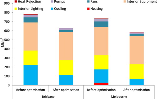
Figure 10 shows the building annual energy consumption and the breakdown of energy consumption before and after optimization for Brisbane and Melbourne for the best solutions found. After applying the optimization method, the annual energy use was reduced by $20.9\mathrm{\%}$ and $19.7\mathrm{\%}$ for Melbourne and Brisbane, respectively. Comparison of energy breakdown between non-optimized and optimized building shows that optimization has significantly reduced the fan energy use (approximately 61%) and cooling load (approximately 20%) for both cities. The fan energy use was reduced $34.6\text{MJ}/{\text{m}}^2$ and $37.9\text{MJ}/{\text{m}}^2$ for Brisbane and Melbourne, respectively. The cooling load dropped $109.8\text{MJ}/{\text{m}}^2$ and $76.8\text{MJ}/{\text{m}}^2$ for Brisbane and Melbourne, respectively.

Figure 10. Breakdown of energy consumption before and after optimization

It is noteworthy that despite the use of daylighting control, lighting loads almost remain unchanged before and after optimization. The reason is that minimizing the lighting and cooling loads is a conflicting objective, therefore, the optimization algorithm prioritizes reduction of the cooling loads. As the optimization algorithm seeks the best balance between the various building loads, it is more likely that an attempt to further reduce the cooling or lighting load would lead to a corresponding increase of equal or greater magnitude in the other.

5. Conclusion

In this research, a new surrogate model-based optimization method using active learning, called L-SOAS, was developed and compared with both the surrogate model-based optimization method using random sampling, and simulation-based optimization (EnergyPlus-in-the-loop). For the simulation-based optimization, two algorithms: PSOIW and ACOR were used as benchmarks.

The results indicated that the new sampling strategy improves the performance of the surrogate model in terms of number of required samples (i.e. simulations) and optimization results. The comparison of results showed that all surrogate-model based optimization methods achieve better results than simulation-based optimization using PSO algorithm implemented in GenOpt software in terms of optimality and computational time (i.e. lower number of simulation calls). However, surrogate model-based optimization and simulation-based optimization with ACO are very competitive. While the simulation-based optimization method using ACOR found better results in terms of optimality at the final optimization stages, the proposed surrogate model-based optimization method showed a better performance at the early optimization stages, yielding solutions within 1% of the best solution found in the fewest number of simulations (about 200 fewer simulations in the Brisbane case study). These results demonstrate the potential for active learning methods to improve the efficiency and accuracy of surrogate model-based optimization methods for BOPs.

From an energy point of view, results showed that after applying optimization methods to a typical medium-size commercial building, approximately $20\mathrm{\%}$ energy savings were achieved for both Brisbane and Melbourne. A comparison of energy breakdown between optimized and non-optimized building showed that cooling load and fan energy use experienced the largest energy reductions for both cities.

The proposed method demonstrates its potential to improve the performance of surrogate model-based optimization methods. In this study, ANNs were selected to create the surrogate model, however, the proposed method can be applied to other surrogate modelling approaches such as radial basis functions. Also, future work should extend to other possible active learning strategies to further improve the performance of surrogate-model based optimization methods especially at the later stages of optimization as well as multi-objective optimization problems.

Acknowledgement

Computational resources and services used in this work were provided by the HPC and Research Support Group, Queensland University of Technology, Brisbane, Australia.

Disclosure statement

No potential conflict of interest was reported by the author(s).

Correction Statement

This article has been republished with minor changes. These changes do not impact the academic content of the article

References

- Asadi, E., M. G. D. Silva, C. H. Antunes, L. Dias, and L. Glicksman. 2014. “Multi-objective Optimization for Building Retrofit: A Model Using Genetic Algorithm and Artificial Neural Network and an Application.” Energy and Buildings 81: 444–456.
- Ascione, F., N. Bianco, C. De Stasio, G. M. Mauro, and G. P. Vanoli. 2017. “Artificial Neural Networks to Predict Energy Performance and Retrofit Scenarios for any Member of a Building Category: A Novel Approach.” Energy 118: 999–1017.
- Attia, S., M. Hamdy, L. William O'Brien, and S. Carlucci. 2013. “ Computational Optimization for Zero Energy Buildings Design: Interview Results with Twenty-Eight International Experts.” In 13th Conference of International Building Performance Simulation Association, Chambéry, France.
- Bamdad, K., M. E. Cholette, L. Guan, and J. Bell. 2017a. Building Energy Retrofits Using ant Colony Optimisation, in Healthy Buildings 2017 Europe. Lublin: International Society of Indoor Air Quality and Climate.
- Bamdad, K., M. E. Cholette, L. Guan, and J. Bell. 2017b. “Ant Colony Algorithm for Building Energy Optimisation Problems and Comparison with Benchmark Algorithms.” Energy and Buildings 154 (Supplement C): 404–414.
- Bamdad, K., M. E. Cholette, L. Guan, and J. Bell. 2018. “Building Energy Optimisation Under Uncertainty Using ACOMV Algorithm.” Energy and Buildings 167: 322–333.
- Bamdad, K., Y. Ma, M.E. Cholette, and J. Bell, 2019. “ Optimisation of HVAC systems using ACOr algorithm, in The Future of HVAC 2019 Conference.” The Australian Institute of Refrigeration, Air Conditioning and Heating Brisbane, Australia.
- Bamdad Masouleh, K. 2018b. Building Energy Optimisation Using Machine Learning and Metaheuristic Algorithms. Brisbane: Queensland University of Technology. https://eprints.qut.edu.au/120281/.
- Bamdad Masouleh, K., M.E. Cholette, L. Guan, and J. Bell, 2017c. “ Building Energy Optimisation Using Artificial Neural Network and Ant Colony Optimisation.” In AIRAH and IBPSA's Australasian Building Simulation 2017 Conference, Melbourne, VIC.
- Board, A.B.C. 2002a. ABCB Energy Modelling of Office Buildings For Climate Zoning (Class 5 Climate Zoning Consultancy) Stages 1, 2 & 3. Melbourne, Victoria: Australian Building Codes Board.
- Board, A.B.C. 2002b. ABCB Energy Modelling of Office Buildings For Climate Zoning (Class 5 Climate Zoning Consultancy) Stages 4 & 5. Melbourne, Victoria: Australian Building Codes Board.
- Brownlee, A. E. I., and J. A. Wright. 2015. “Constrained, Mixed-Integer and Multi-Objective Optimisation of Building Designs by NSGA-II with Fitness Approximation.” Applied Soft Computing 33: 114–126.
- Bui, Lam T., Omar Soliman, and Hussein A. Abbass. 2007. “A Modified Strategy for the Constriction Factor in Particle Swarm Optimization.” Lecture Notes in Computer Science 4828: 333–344.
- Chou, J.-S., and D.-K. Bui. 2014. “Modeling Heating and Cooling Loads by Artificial Intelligence for Energy-Efficient Building Design.” Energy and Buildings 82: 437–446.
- Cohn, D. A., Z. Ghahramani, and M. I. Jordan. 1996. “Active Learning with Statistical Models.” J. Artif. Int. Res 4 (1): 129–145.
- Conraud-Bianchi, J. 2008. A Methodology for the Optimization of Building Energy, Thermal, and Visual Performance. Montréal, Québec: Concordia University.
- Demuth, H., M. Beale, and M. Hagan. 2006. Neural Network Toolbox 6 for User's Guide. Natick, Massachusetts: The MathWorks, Inc.
- Dorigo, M., V. Maniezzo, and A. Colorni. 1996. “Ant System: Optimization by a Colony of Cooperating Agents. Systems, Man, and Cybernetics, Part B: Cybernetics.” IEEE Transactions on 26 (1): 29–41.
- Eisenhower, B., Z. O’Neill, S. Narayanan, V. A. Fonoberov, and I. Mezić. 2012. “A Methodology for Meta-Model Based Optimization in Building Energy Models.” Energy and Buildings 47: 292–301.
- EnergyPlus Energy Simulation Software. 2015. http://apps1.eere.energy.gov/buildings/energyplus/.
- Evins, R. 2013. “A Review of Computational Optimisation Methods Applied to Sustainable Building Design.” Renewable and Sustainable Energy Reviews 22: 230–245.
- Gengembre, E., B. Ladevie, O. Fudym, and A. Thuillier. 2012. “A Kriging Constrained Efficient Global Optimization Approach Applied to low-Energy Building Design Problems.” Inverse Problems in Science and Engineering 20 (7): 1101–1114.
- Gilan, S., N. Goyal, and B. Dilkina. 2016. Active Learning in Multi-Objective Evolutionary Algorithms for Sustainable Building Design. New York: Association for Computing Machinery. doi.org/10.1145/2908812.2908947.
- Gossard, D., B. Lartigue, and F. Thellier. 2013. “Multi-objective Optimization of a Building Envelope for Thermal Performance Using Genetic Algorithms and Artificial Neural Network.” Energy and Buildings 67: 253–260.
- Haykin, S. 1998. Neural Networks: A Comprehensive Foundation. Upper Saddle River, New Jersey: Prentice Hall PTR.
- Haykin, S. S. 2009. Neural Networks and Learning Machines, Vol. 3. Upper Saddle River, NJ: Pearson .
- Hornik, K., M. Stinchcombe, and H. White. 1989. “Multilayer Feedforward Networks are Universal Approximators.” Neural Networks 2 (5): 359–366.
- Jin, Y. 2005. “A Comprehensive Survey of Fitness Approximation in Evolutionary Computation.” Soft Computing 9 (1): 3–12.
- Jin, Y. 2011. “Surrogate-assisted Evolutionary Computation: Recent Advances and Future Challenges.” Swarm and Evolutionary Computation 1 (2): 61–70.
- Kämpf, J. H., M. Wetter, and D. Robinson. 2010. “A Comparison of Global Optimization Algorithms with Standard Benchmark Functions and Real-World Applications Using EnergyPlus.” Journal of Building Performance Simulation 3 (2): 103–120.
- Kecman, V. 2001. Learning and Soft Computing: Support Vector Machines, Neural Networks, and Fuzzy Logic Models. Cambridge, Massachusetts: MIT Press.
- Kohavi, R., 1995. “ A Study of Cross-validation and Bootstrap for Accuracy Estimation and Model Selection.” In Proceedings of the 14th international joint conference on Artificial intelligence - Volume 2. 1995, Morgan Kaufmann Publishers Inc.: Montreal, Quebec, Canada. p. 1137-1143.
- Krogh, A., and J. Vedelsby. 1995. “Neural Network Ensembles, Cross Validation, and Active Learning.” Advances in Neural Information Processing Systems 7: 231–238.
- Kůrková, V. 1992. “Kolmogorov's Theorem and Multilayer Neural Networks.” Neural Networks 5 (3): 501–506.
- Liu, H., Y.-S. Ong, and J. Cai. 2018. “A Survey of Adaptive Sampling for Global Metamodeling in Support of Simulation-Based Complex Engineering Design.” Structural and Multidisciplinary Optimization 57 (1): 393–416.
- Magnier, L., and F. Haghighat. 2010. “Multiobjective Optimization of Building Design Using TRNSYS Simulations, Genetic Algorithm, and Artificial Neural Network.” Building and Environment 45 (3): 739–746.
- Mba, L., P. Meukam, and A. Kemajou. 2016. “Application of Artificial Neural Network for Predicting Hourly Indoor air Temperature and Relative Humidity in Modern Building in Humid Region.” Energy and Buildings 121 (Supplement C): 32–42.
- McCulloch, W., and W. Pitts. 1943. “A Logical Calculus of the Ideas Immanent in Nervous Activity.” The Bulletin of Mathematical Biophysics 5 (4): 115–133.
- McKay, M. D., R. J. Beckman, and W. J. Conover. 1979. “Comparison of Three Methods for Selecting Values of Input Variables in the Analysis of Output From a Computer Code.” Technometrics 21 (2): 239–245.
- Meckesheimer, M., A. J. Booker, R. R. Barton, and T. W. Simpson. 2002. “Computationally Inexpensive Metamodel Assessment Strategies.” AIAA Journal 40 (10): 2053–2060.
- Melo, A. P., R. S. Versage, G. Sawaya, and R. Lamberts. 2016. “A Novel Surrogate Model to Support Building Energy Labelling System: A new Approach to Assess Cooling Energy Demand in Commercial Buildings.” Energy and Buildings 131: 233–247.
- National Australian Built Environment Rating Scheme. 2011. NABERS Energy Guide to Building Energy Estimation.
- Neto, A. H., and F. A. S. Fiorelli. 2008. “Comparison Between Detailed Model Simulation and Artificial Neural Network for Forecasting Building Energy Consumption.” Energy and Buildings 40 (12): 2169–2176.
- Nguyen, A.-T., S. Reiter, and P. Rigo. 2014. “A Review on Simulation-Based Optimization Methods Applied to Building Performance Analysis.” Applied Energy 113: 1043–1058.
- Østergård, T., R. L. Jensen, and S. E. Maagaard. 2018. “A Comparison of six Metamodeling Techniques Applied to Building Performance Simulations.” Applied Energy 211: 89–103.
- Pang, Z., Z. O'Neill, Y. Li, and F. Niu. 2020. “The Role of Sensitivity Analysis in the Building Performance Analysis: A Critical Review.” Energy and Buildings 209: 109659.
- Roman, N. D., F. Bre, V. D. Fachinotti, and R. Lamberts. 2020. “Application and Characterization of Metamodels Based on Artificial Neural Networks for Building Performance Simulation: A Systematic Review.” Energy and Buildings 217: 109972.
- Romero, David, José Rincón, and Nastia Almao. 2001. “Optimization of the thermal behavior of tropical buildings.” Seventh International IBPSA Conference, Rio de Janeiro, Brazil.
- Settles, B. 2012. Active Learning. San Rafael, California: Morgan & Claypool Publishers.
- Socha, K., and M. Dorigo. 2008. “Ant Colony Optimization for Continuous Domains.” European Journal of Operational Research 185 (3): 1155–1173.
- Tresidder E, Y.Z. I. Alexander.J. Forrester, 2011. “ Optimisation of Low-Energy Building Design Using Surrogate Models.” In 12th Conference of International Building Performance Simulation Association, Sydney.
- Tresidder, E., Y. Z. Alexander, and J. Forrester. 2012. “ Acceleration of Building Design Optimisation Through the Use of Kriging Surrogate Models.” In Proceedings of building simulation and optimization Loughborough University, Loughborough, Leicestershire.
- UNEP, Buildings and Climate Change Summary for Decision-Makers. 2009. France. http://www.unep.org/sbci/pdfs/SBCI-BCCSummary.pdf.
- Ürge-Vorsatz, D., L. F. Cabeza, S. Serrano, C. Barreneche, and K. Petrichenko. 2015. “Heating and Cooling Energy Trends and Drivers in Buildings.” Renewable and Sustainable Energy Reviews 41: 85–98.
- Waibel, C., T. Wortmann, R. Evins, and J. Carmeliet. 2019. “Building Energy Optimization: An Extensive Benchmark of Global Search Algorithms.” Energy and Buildings 187: 218–240.
- Westermann, P., and R. Evins. 2019. “Surrogate Modelling for Sustainable Building Design – A Review.” Energy and Buildings 198: 170–186.
- Wetter, M., and J. Wright. 2004. “A Comparison of Deterministic and Probabilistic Optimization Algorithms for Nonsmooth Simulation-Based Optimization.” Building and Environment 39 (8): 989–999.
- Wortmann, T. 2019. “Genetic Evolution vs. Function Approximation: Benchmarking Algorithms for Architectural Design Optimization.” Journal of Computational Design and Engineering 6 (3): 414–428.
- Zemella, G., D. De March, M. Borrotti, and I. Poli. 2011. “Optimised Design of Energy Efficient Building Façades via Evolutionary Neural Networks.” Energy and Buildings 43 (12): 3297–3302.
- Zhang, R., F. Liu, A. Schörgendorfer, Y. Hwang, Y. M. Lee, and J. L. Snowdon. 2013. Optimal Selection of Building Components Using Sequential Design via Statistical Surrogate Models.