On modelling effects in the battery and thermal storage scheduling problem

ABSTRACT

The growing use of intermittent renewable energy sources requires an increased amount of storage capacity to match uncertain generation with uncertain demand. A possible solution is the use of thermal and electrical storages. This paper compares several model formulations: mixed integer linear programs (MILPs), nonlinear programs (NLPs), mixed integer nonlinear programs (MINLPs) for optimizing the operation of a multi-modal home energy system comprising heating and electricity subsystems. The respective optimization problems are then resolved within a model predictive control scheme and the final solutions are compared in terms of runtime and optimality. The results indicate that a thermocline-based thermal storage model leads to the overall lowest costs while not significantly impeding computing times. Additionally, the results show that a continuous heat pump model leads to reduced computing times without affecting the modelling accuracy.

Keywords:

• Thermal storages
• battery scheduling
• model predictive control
• mixed integer optimization
• nonlinear optimization
• modelling

1. Introduction

The growing use of intermittent renewable energy sources has created substantial technical, economic and political challenges. One challenge of particular prominence and importance is the problem of matching uncertain generation with uncertain demand. A possible solution is the use of thermal and electrical storages, which effectively allows for shifting available generation to meet demand (Setlhaolo, Sichilalu, and Zhang 2017; Appino et al. 2018). In this work, we concentrate on local storages within buildings, with a particular focus on batteries and hot water storage tanks. Considering the complexity of such distributed, multi-modal energy systems, optimization methods present a viable option for controlling such systems.

1.1. Model predictive control

The optimization of distributed, multi-modal energy systems requires forecasting upcoming thermal and electrical demands, setting up an optimization model that represents the energy system and then solving the optimization model, resulting in control signals that are sent to the systems actuators, e.g. charging a battery, curtailing a photovoltaic array or activating a heat pump. Since each of these steps introduces errors, such as forecasting errors and modelling errors, Model Predictive Control (MPC) is typically applied to such control problems.

The MPC approach has been in use since the 1980s and has a well-developed theory (Kwon, Bruckstein, and Kailath 1983; Mayne et al. 2000; Qin and Badgwell 2003). The main idea of MPC is to perform a receding horizon optimal control strategy such that the best controller input over a finite horizon is calculated but only the current time step is implemented. Afterwards, the state is updated and the process repeats for the remaining time steps. This allows for the consideration of future events and real-time flexibility. It is also well known that each new optimization horizon can adjust for some inaccuracies (Garcia, Prett, and Morari 1989). Many practical applications such as battery scheduling problems (Arnold and Andersson 2011), torque control (Geyer 2009) and building control (Maasoumy et al. 2014) involve nonlinear effects but the models used in MPC are most frequently only linear. The success of MPC in these applications derives in part from the fact that even though the dynamics of the systems in question are nonlinear, they are approximately linear over sufficiently short time periods, and thus a linear model that is continuously adjusted by empirical data can allow for robust control while still guaranteeing some notion of optimality. There are different approaches to model energy systems in such MPC control models.

1.2. Energy system modelling

Considering local storages within buildings, both batteries and hot water tanks have dynamics which are inherently non-linear and thus are generally not accurately modelled via linear equations. However, the degree to which they are inaccurate is only evaluated for static operation (Oliveski, Krenzinger, and Vielmo 2003).

While simulation software typically discretizes hot water storage tanks into multiple vertical layers (Oliveski, Krenzinger, and Vielmo 2003), MPC models follow different approaches. Most commonly, thermal storage units are modelled as thermal capacities that are perfectly mixed and are represented by their homogeneously distributed internal energy (Collazos, Maréchal, and Gähler 2009; Ashouri et al. 2013; Wakui and Yokoyama 2014; D'Ettorre et al. 2019). This approach therefore neglects thermal stratification that is inherent to these components. Only a few studies tried to represent thermal stratification in mixed-integer linear programs. In Fazlollahi, Becker, and Marchal (2014), the authors assume the temperatures in the top and bottom layers in their storage model as parameters. Within the optimization model, they discretize the temperature difference and compute the resulting volumes of each layer (Fazlollahi, Becker, and Marchal 2014). This approach is able to compute the stratification inside the storage, but in most applications, the temperature levels are decision variables of the optimization problem which cannot be computed with this model. Steen et al. (2015) propose to implement two simple storage models to represent a high temperature (HT) and a low temperature (LT) section within the storage tank. Their model is able to account for the charging of the LT section with HT fluid, but does not consider LT fluid flowing into the HT section if the HT section is discharged.

Similar to hot water storage tanks, there exist different approaches to model battery storages. There exist nonlinear approaches to model effects such as preventing a simultaneous charging and discharging of the battery (Appino et al. 2018). Alternatively, Murray, Faulwasser, and Hagenmeyer (2018); Sass et al. (2020) illustrate how such nonlinear battery models can be reformulated with mixed-integer linear approaches. In Bösenberg et al. (2015), it is shown that higher cycling rates can reduce battery lifetime, and thus a controller which avoids this can reduce long term maintenance costs. Smart metering is a highly related topic to battery control and some research has shown that levelling the power profile can help to obscure local load profiles from a centralized controller Yang et al. (2014).

1.3. Contribution

As previously mentioned, there exist a number of approaches that seek to solve the optimal control problem of distributed, multi-modal energy systems. Each approach utilizes different models and solution methods, but to date there has been no analysis of how best to formulate and solve this problem. The various combinations of modelling choices result in non-linear, mixed-integer linear and mixed-integer nonlinear systems. The main contribution of the present paper is to provide some insight as to which components of the Battery and Thermal Storage Scheduling (BATSS) problem should be modelled with linear dynamics and which require more complex modelling.

This paper is organized as follows: Section 2 proposes a number of different modelling alternatives for the combined battery and thermal storage scheduling problem. Section 3 solves the problems posed in Section 2 using state-of-the-art solution methods and these results are discussed in Section 4. Finally, Section 5 discusses the results of Section 3 and provides an outlook on possible future research directions.

2. Models

Although there is no standard formulation of the BATSS problem, any formulation will share a number of common features. Namely, there is a cost for total power used, heat pump, thermal storage, electric battery and some coupling of the subsystems. There may be multiple storages and loads, but we will restrict our analysis to the case of a single household (i.e. a heat pump, battery and thermal storages for both domestic hot water and space heating use). All conclusions based on the analysis of the single house case should apply to BATSS problem for multiple households as the form of the problem does not change, except for a linear coupling of the households.

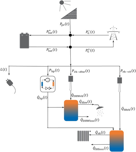
Sections 2.1– 2.5 give detailed descriptions of each of the major components of the model, which is summarized in Figure 1.

Figure 1. Schematic diagram of the system to be optimized.

2.1. Model of connection to main grid

The primary objective of any BATSS problem is to minimize electricity costs. Let the power fed into the main grid at time t be denoted by $P_G^{+}(t)\ge 0$ and the power drawn from the grid at that time step be likewise denoted by $P_G^{-}(t)\le 0$. Let the revenue per kW from feed-in at time t be denoted by $c^{+}(t)\ge 0$ and the cost of purchasing from the grid at time t by $c^{-}(t)\le 0$. The objective of minimizing electricity costs over the discretized time horizon $t\in \{1,\dots ,H\}$ can then be formulated as (1) $\begin{array}{r}max\sum _{t=1}^H(c^{+}(t)P_G^{+}(t)-c^{-}(t)P_G^{-}(t)){\mathrm{\Delta }}_t\end{array}$(1) where ${\mathrm{\Delta }}_t$ is the length of each time step. In principle, it is possible for the solution to contain both $P_G^{+}(t)>0$ and $P_G^{-}(t)>0$ for some time step t. To avoid this, one can use complementarity constraints. These may be formulated exactly as mixed-integer linear inequality constraints (Equation (2(2) $\begin{array}{rl}0\le P_G^{+}(t)& \le (1-z(t)){\overline{P}}_G\\ z(t){\underset{\_}{P}}_G\le P_G^{-}(t)& \le 0\\ \mathrm{where}z(t)& \in \{0,1\}\end{array}$(2) )) or inexactly via the continuous-valued nonlinear Fischer–Burmeister relaxation (Fischer 1992) (Equation (3(3) $\begin{array}{rl}0\le P_G^{+}(t)& \le {\overline{P}}_G\\ {\underset{\_}{P}}_G\le P_G^{-}(t)& \le 0\\ ϵ\le P_G^{+}(t)P_G^{-}(t)& \le 0\\ \mathrm{for}\mathrm{some}ϵ& <0\end{array}$(3) )): (2) $\begin{array}{rl}0\le P_G^{+}(t)& \le (1-z(t)){\overline{P}}_G\\ z(t){\underset{\_}{P}}_G\le P_G^{-}(t)& \le 0\\ \mathrm{where}z(t)& \in \{0,1\}\end{array}$(2) (3) $\begin{array}{rl}0\le P_G^{+}(t)& \le {\overline{P}}_G\\ {\underset{\_}{P}}_G\le P_G^{-}(t)& \le 0\\ ϵ\le P_G^{+}(t)P_G^{-}(t)& \le 0\\ \mathrm{for}\mathrm{some}ϵ& <0\end{array}$(3) where ${\overline{P}}_G$ and ${\underset{\_}{P}}_G$ are the upper and lower bounds on the power to/from the grid. A tighter Fischer–Burmeister relaxation (i.e., where ε is closer to 0) will result in more accurate solutions, but runs the risk of numerical issues for some solution methods.

As the cost of buying electricity from the main grid typically differs from the price of selling electricity to the grid, an integer decision variable can be used to differentiate between these two cases and enforce a complementarity constraint between them. Alternatively, absolute value functions may be used, but this would imply solving a real-valued Nonlinear Program (NLP) instead of a Mixed Integer Linear Program (MILP). As shown in Murray, Faulwasser, and Hagenmeyer (2018), the latter generally gives better results for the BATSS problem (Table 1).

Table 1. Grid connection parameters. Based on most recent values for private households in Western Germany.

Electricity Tariff	$c^{-}(t)$	0.30 $/kWh${}^{\mathrm{a}}$
Remuneration for feed-in	$c^{+}(t)$	0.11 $/kWh${}^{\mathrm{b}}$

${}^{\mathrm{a}}$www.destatis.de/DE/Publikationen/Thematisch/Preise/Energiepreise/EnergiepreisentwicklungPDF_5619001.pdf

${}^{\mathrm{b}}$www.bundesnetzagentur.de/SharedDocs/Downloads/DE/Sachgebiete/Energie/Unternehmen_Institutionen/ErneuerbareEnergien/ZahlenDatenInformationen/PV_Datenmeldungen/DegressionsVergSaetze_08-10_18.xlsx?_blob=publicationFile&v=2

2.2. Models of heat pump

One of the major components of the battery and thermal storage system is the heat pump. It is a device that uses electricity to heat water for domestic hot water or space heating usage or for charging either of the thermal storage tanks. We consider a two-point controlled air-to-water heat pump. Using different set-temperatures for domestic hot water and space heating results in three discrete operating modes for each time step, depending on whether it is providing water for domestic or space heating use¹, or neither. Thus an integer decision variable is used to model this choice. More information on heat pumps can be found in Langley (2002); Grassi (2017).

Equations:

• Power usage of heat pump

  $P_{hp}(t)=P_{dhw}{y}_{dhw}(t)+P_{sh}{y}_{sh}(t)$

• Heat output

  $Q_{hp}(t)=\mu (t,T)P_{hp}(t)$

• Only choose one temperature setting

  $y_{dhw}(t)+y_{sh}(t)\le 1$

Thereby $P_{dhw}$ and $P_{sh}$ are the power usages of the heat pump for water at 60${}^{\circ }$C and 35 ${}^{\circ }$C, respectively. Likewise, $y_{dhw}$ and $y_{sh}$ are the controls associated with each of these temperature outputs (cf. Table 2). The heat added to the thermal storage tanks is denoted by $Q_{hp}$, where the coefficient of performance (COP) $\mu (t,T)$ depends on the environment temperature at time t and desired output temperature T. For the domestic hot water tank, this is 60 ${}^{\circ }$, and 35 for the space heating tank. If a temperature forecast is given, then these coefficients can be precomputed. The ambient temperature and heating demand are shown in Figure 2, and the temperature-dependent COP for the investigated heat pump is illustrated in Figure 3. Thereby, the blue curve depicts the COP when providing heat for space heating and the red curve shows the COP for domestic hot water provision.

Figure 2. Ambient temperature data taken from Deutscher Wetterdienst (2017). The time frame spans several days in spring in Aachen. The solid red line is the ambient temperature, the dotted blue line is the domestic hot water demand and the dashed green line is the space heating demand.

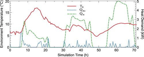
Figure 3. Collected data for the coefficient of performance for a given heat pump Dimplex with a linear interpolation. The solid blue line denotes the COP given the required $60\mathrm{deg}$ output for the domestic hot water tank. Likewise, the dashed red line denotes the COP for the $35\mathrm{deg}$ required by the space heating tank.

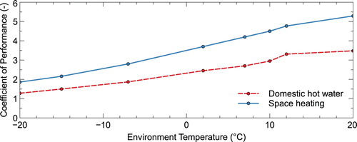
Table 2. Heat pump parameters. Technical data based on Dimplex LA 12TU heat pump Dimplex.

Coefficient of performance (domestic hot water)	$\mu (t,60)$	See Figure 3
Coefficient of performance (space heating)	$\mu (t,35)$	See Figure 3
Power usage for heating domestic hot water	$P_{dhw}$	3.75 kW
Power usage for space heating	$P_{sh}$	2.5 kW

While the heat pump has discrete settings, one may require these to be applied for the entire time step or just for a fraction. In the first case, the control decisions $y_{dhw}$ and $y_{sh}$ will be discrete valued and in the second case, they will be continuous. Both cases are shown in Equations (4(4) $\begin{array}{rl}& y_{dhw}(t)\in \{0,1\},\mathrm{\forall }t\end{array}$(4) ) and (5(5) $\begin{array}{rl}& 0\le y_{dhw}(t)\le 1,\mathrm{\forall }t\end{array}$(5) ): (4) $\begin{array}{rl}& y_{dhw}(t)\in \{0,1\},\mathrm{\forall }t\end{array}$(4) (5) $\begin{array}{rl}& 0\le y_{dhw}(t)\le 1,\mathrm{\forall }t\end{array}$(5) The advantage of (4(4) $\begin{array}{rl}& y_{dhw}(t)\in \{0,1\},\mathrm{\forall }t\end{array}$(4) ) is that the solution is clear and well-defined, however, it can lead to some inefficiency due to overcharging. For (5(5) $\begin{array}{rl}& 0\le y_{dhw}(t)\le 1,\mathrm{\forall }t\end{array}$(5) ), the precise amount of heating can be applied, but the exact time when the heatpump is activated is unclear. One could define the activation to always be from the beginning of the time step, however for multiple time steps with partial activations this could lead to cycling losses or increased maintenance costs to sequences of short activations.

2.3. Models of thermal storage tanks

Typically, simulation software discretizes thermal energy storages into multiple segments (nodes) in the vertical direction (Powell and Edgar 2013). Each node has a certain temperature and water mass. The temperature of the tank is constantly losing thermal energy to the environment, based on tank parameters (shown in Table 3) and ambient temperature (shown in Figure 2). Furthermore, if the storage is discharged, a net flow from the bottom to the top mixes the storage and vice versa during charging events. Thereby, the top and bottom segments have the largest surface areas; therefore, the top segment can become colder than the second-to-the-top segment in such simulation models. This is not a physical phenomenon; thus simulation software typically sorts the segments after each time-discrete step or at least performs a mixing (Oliveski, Krenzinger, and Vielmo 2003).

Table 3. Thermal storage tank parameters.

Diameter of domestic hot water storage	$d_{dhw}$	0.45 m
Diameter of space heating water storage	$d_{sh}$	0.79 m
Height of domestic hot water storage	$h_{dhw}$	0.75 m
Height of space heating water storage	$h_{sh}$	2 m
Volume of domestic hot water storage	$V_{dhw}$	0.12 ${\mathrm{m}}^3$
Volume of space heating water storage	$V_{sh}$	0.98 ${\mathrm{m}}^3$
Area of lid of domestic hot water storage	$A_{dhw}$	0.16 ${\mathrm{m}}^2$
Area of lid of space heating water storage	$A_{sh}$	0.49 ${\mathrm{m}}^2$
Set-point for flow temperature for domestic hot water	$T_{dhw}$	60${}^{\circ }$C
Set-point for flow temperature for space heating	$T_{sh}$	35${}^{\circ }$C
Temperature of water pumped into storage	$T_{\ell }$	25${}^{\circ }$C
Temperature of environment	$T_R(t)$	See Figure 2
Specific heat capacity of water	c	4.1796 kJ/(kg K)
Density of water	ρ	997 $\mathrm{kg}/{\mathrm{m}}^3$
Thermal conductivity of water	k	0.64 W/mK
Coefficient of heat losses	U	0.617 $\mathrm{W}/{\mathrm{m}}^2\mathrm{K}$
Time step length	${\mathrm{\Delta }}_t$	30 min${}^{\mathrm{a}}$
Building's (space heating/domestic hot water) demand	$m(t)$	See Figure 2
Efficiency of electric heater for DHW tank	${\epsilon }_{DHWeh}$	1
Efficiency of electric heater for SH tank	${\epsilon }_{SHeh}$	1

${}^{\mathrm{a}}$ The time step length was chosen to be 30 minutes due to the granularity of the available data sets.

However, simulation of the thermal storage tanks in such granularity is not necessarily useful nor practical in embedded systems. Herein we shall assume that temperature readings $T_1$, $T_2$ and $T_3$ are available. These correspond to the temperature of the water at the bottom, middle and top of the tank, respectively. Given this information, one way to model the state X of a tank is by using two nodes: the section of the tank with water at a usable temperature and the section with low, unusable temperature. This ‘thermocline’ model is depicted in Equation (7(7) $\begin{array}{rl}& \rho Vc(X(t+1)-X(t))/{\mathrm{\Delta }}_t\\ & =-m(t)(T_1-T_R(t))/c(T_{ts}-T_R(t))\\ & +((Q_{eh}(t)+Q_{hp}(t)\\ & -UA(T_1+T_2-2T_R(t))\\ & -U\pi dh(T_1-T_R(t)))/(T_{ts}-T_R(t)).\end{array}$(7) ). Another option is to model X as the total energy content of the tank as shown in Equation (6(6) $\begin{array}{rl}& \rho Vc(X(t+1)-X(t))/{\mathrm{\Delta }}_t\\ & =-m(t)/c+(Q_{eh}(t)+Q_{hp}(t)\\ & -UA(T_1+T_3-2T_R(t))\\ & -U\pi dh(T_2-T_R(t)))/(T_{ts}-T_3).\end{array}$(6) ). Doing so may be a poor choice if the temperature difference between the bottom and top of the tank is no longer very large, but can be more accurate if the water temperature in the top of the tank greatly exceeds the fixed temperature assumed in the thermocline model. In other words, if the hot water tank is charged a lot in a short period of time, then Equation (6(6) $\begin{array}{rl}& \rho Vc(X(t+1)-X(t))/{\mathrm{\Delta }}_t\\ & =-m(t)/c+(Q_{eh}(t)+Q_{hp}(t)\\ & -UA(T_1+T_3-2T_R(t))\\ & -U\pi dh(T_2-T_R(t)))/(T_{ts}-T_3).\end{array}$(6) ) will likely be more accurate while a long period without charging will result in the usable water being more accurately modelled by Equation (7(7) $\begin{array}{rl}& \rho Vc(X(t+1)-X(t))/{\mathrm{\Delta }}_t\\ & =-m(t)(T_1-T_R(t))/c(T_{ts}-T_R(t))\\ & +((Q_{eh}(t)+Q_{hp}(t)\\ & -UA(T_1+T_2-2T_R(t))\\ & -U\pi dh(T_1-T_R(t)))/(T_{ts}-T_R(t)).\end{array}$(7) ). Of course, the nonlinear dynamics of the thermal storages may be explicitly modelled as in Equation (8(8) $\begin{array}{rl}& \rho Vc(T_2(t+1)-T_2(t))/{\mathrm{\Delta }}_t\\ & =m(t)/c(T_3(t)-T_2(t))\\ & +Q_{hp}(t)(T_1(t)-T_2(t))/(T_{ts}-T_3(t))\\ & -U\pi dh(T_2(t)-T_R(t))\\ & +kA(T_3(t)+T_1(t)-2T_2(t))/0.2\mathrm{h}\end{array}$(8) ), however, doing so may lead to longer runtimes. Section 4 will present the results of each of these thermal storage models in combination with several other modelling options for the system.

The dynamics of thermal storage dynamics involve a number of parameters, which are given in Table 3. Note that the subscripts dhw and sh are omitted in (6(6) $\begin{array}{rl}& \rho Vc(X(t+1)-X(t))/{\mathrm{\Delta }}_t\\ & =-m(t)/c+(Q_{eh}(t)+Q_{hp}(t)\\ & -UA(T_1+T_3-2T_R(t))\\ & -U\pi dh(T_2-T_R(t)))/(T_{ts}-T_3).\end{array}$(6) ), (7(7) $\begin{array}{rl}& \rho Vc(X(t+1)-X(t))/{\mathrm{\Delta }}_t\\ & =-m(t)(T_1-T_R(t))/c(T_{ts}-T_R(t))\\ & +((Q_{eh}(t)+Q_{hp}(t)\\ & -UA(T_1+T_2-2T_R(t))\\ & -U\pi dh(T_1-T_R(t)))/(T_{ts}-T_R(t)).\end{array}$(7) ) and (8(8) $\begin{array}{rl}& \rho Vc(T_2(t+1)-T_2(t))/{\mathrm{\Delta }}_t\\ & =m(t)/c(T_3(t)-T_2(t))\\ & +Q_{hp}(t)(T_1(t)-T_2(t))/(T_{ts}-T_3(t))\\ & -U\pi dh(T_2(t)-T_R(t))\\ & +kA(T_3(t)+T_1(t)-2T_2(t))/0.2\mathrm{h}\end{array}$(8) ) for brevity, as the same dynamics hold for each tank.

1. Energy state dynamics (6) $\begin{array}{rl}& \rho Vc(X(t+1)-X(t))/{\mathrm{\Delta }}_t\\ & =-m(t)/c+(Q_{eh}(t)+Q_{hp}(t)\\ & -UA(T_1+T_3-2T_R(t))\\ & -U\pi dh(T_2-T_R(t)))/(T_{ts}-T_3).\end{array}$(6) 2. Thermocline between usable and unusable water (7) $\begin{array}{rl}& \rho Vc(X(t+1)-X(t))/{\mathrm{\Delta }}_t\\ & =-m(t)(T_1-T_R(t))/c(T_{ts}-T_R(t))\\ & +((Q_{eh}(t)+Q_{hp}(t)\\ & -UA(T_1+T_2-2T_R(t))\\ & -U\pi dh(T_1-T_R(t)))/(T_{ts}-T_R(t)).\end{array}$(7) 3. Nonlinear thermocline model. Includes the same state dynamics as in Equation (7(7) $\begin{array}{rl}& \rho Vc(X(t+1)-X(t))/{\mathrm{\Delta }}_t\\ & =-m(t)(T_1-T_R(t))/c(T_{ts}-T_R(t))\\ & +((Q_{eh}(t)+Q_{hp}(t)\\ & -UA(T_1+T_2-2T_R(t))\\ & -U\pi dh(T_1-T_R(t)))/(T_{ts}-T_R(t)).\end{array}$(7) ), except that $T_1,T_2,$ and $T_3$ are non-constant and have the following dynamics $\mathrm{\forall }t>0:$ $\begin{array}{rl}& \rho Vc(T_1(t+1)-T_1(t))/{\mathrm{\Delta }}_t\\ & =m(t)/c(T_2(t)-T_1(t))\\ & +Q_{hp}(t)(T_{ts}-T_1(t))/(T_{ts}-T_3(t))\\ & -U\pi dh(T_1(t)-T_R(t))\\ & +kA(T_2(t)-T_1(t)/0.2\mathrm{h}\end{array}$ (8) $\begin{array}{rl}& \rho Vc(T_2(t+1)-T_2(t))/{\mathrm{\Delta }}_t\\ & =m(t)/c(T_3(t)-T_2(t))\\ & +Q_{hp}(t)(T_1(t)-T_2(t))/(T_{ts}-T_3(t))\\ & -U\pi dh(T_2(t)-T_R(t))\\ & +kA(T_3(t)+T_1(t)-2T_2(t))/0.2\mathrm{h}\end{array}$(8) $\begin{array}{rl}& \rho Vc(T_3(t+1)-T_3(t))/{\mathrm{\Delta }}_t\\ & =m(t)/c(T_R(t)-T_3(t))\\ & +Q_{hp}(t)(T_2(t)-T_3(t))/(T_{ts}-T_3(t))\\ & -U\pi dh(T_3(t)-T_R(t))\\ & +kA(T_2(t)-T_3(t))/0.2\mathrm{h}\end{array}$ and where $T_1(0),T_2(0)$ and $T_3(0)$ are the thermal storage temperature readings.

In all three models, the main idea is to equate the change in usable water with the heat added by the heat pump ($Q_{hp}$) and electric heater ($Q_{eh}$), minus the hot water demand (m), and heat lost to the environment. Note that the notation $T_{ts}$ is used refer to the temperature set-point of the thermal storage tank in question. These values are given as $T_{dhw}$ and $T_{sh}$ in Table 3 for the domestic hot water and space heating tanks, respectively. It should also be noted that for Equations (6(6) $\begin{array}{rl}& \rho Vc(X(t+1)-X(t))/{\mathrm{\Delta }}_t\\ & =-m(t)/c+(Q_{eh}(t)+Q_{hp}(t)\\ & -UA(T_1+T_3-2T_R(t))\\ & -U\pi dh(T_2-T_R(t)))/(T_{ts}-T_3).\end{array}$(6) ) and (7(7) $\begin{array}{rl}& \rho Vc(X(t+1)-X(t))/{\mathrm{\Delta }}_t\\ & =-m(t)(T_1-T_R(t))/c(T_{ts}-T_R(t))\\ & +((Q_{eh}(t)+Q_{hp}(t)\\ & -UA(T_1+T_2-2T_R(t))\\ & -U\pi dh(T_1-T_R(t)))/(T_{ts}-T_R(t)).\end{array}$(7) ) the thermoclines X are further constrained by $0\le X(t)\le 1,$ where $X(t)=1$ corresponds to a completely ‘charged’ hot water tank, while $X(t)=0$ would correspond to a tank without any usable hot water.

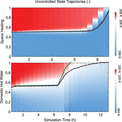
Figure 4 provides an illustrative example of the behaviour of the state X in the dynamics given by (6(6) $\begin{array}{rl}& \rho Vc(X(t+1)-X(t))/{\mathrm{\Delta }}_t\\ & =-m(t)/c+(Q_{eh}(t)+Q_{hp}(t)\\ & -UA(T_1+T_3-2T_R(t))\\ & -U\pi dh(T_2-T_R(t)))/(T_{ts}-T_3).\end{array}$(6) ), (7(7) $\begin{array}{rl}& \rho Vc(X(t+1)-X(t))/{\mathrm{\Delta }}_t\\ & =-m(t)(T_1-T_R(t))/c(T_{ts}-T_R(t))\\ & +((Q_{eh}(t)+Q_{hp}(t)\\ & -UA(T_1+T_2-2T_R(t))\\ & -U\pi dh(T_1-T_R(t)))/(T_{ts}-T_R(t)).\end{array}$(7) ) and (8(8) $\begin{array}{rl}& \rho Vc(T_2(t+1)-T_2(t))/{\mathrm{\Delta }}_t\\ & =m(t)/c(T_3(t)-T_2(t))\\ & +Q_{hp}(t)(T_1(t)-T_2(t))/(T_{ts}-T_3(t))\\ & -U\pi dh(T_2(t)-T_R(t))\\ & +kA(T_3(t)+T_1(t)-2T_2(t))/0.2\mathrm{h}\end{array}$(8) ). Here, the hot water demands and ambient temperature are as given in Table 3, however, no control actions are undertaken. The shaded cells use values taken from a detailed simulation of both tanks. Both the linear and nonlinear models seem to underestimate the heat losses for the thermal storages. Interestingly, the linear model (Equation (6(6) $\begin{array}{rl}& \rho Vc(X(t+1)-X(t))/{\mathrm{\Delta }}_t\\ & =-m(t)/c+(Q_{eh}(t)+Q_{hp}(t)\\ & -UA(T_1+T_3-2T_R(t))\\ & -U\pi dh(T_2-T_R(t)))/(T_{ts}-T_3).\end{array}$(6) )), seems to be the best predictor despite only relying on relatively simple dynamics.

Figure 4. The solid green line is the prediction of Model 1 (Equation (6(6) $\begin{array}{rl}& \rho Vc(X(t+1)-X(t))/{\mathrm{\Delta }}_t\\ & =-m(t)/c+(Q_{eh}(t)+Q_{hp}(t)\\ & -UA(T_1+T_3-2T_R(t))\\ & -U\pi dh(T_2-T_R(t)))/(T_{ts}-T_3).\end{array}$(6) )). The dashed purple line depicts the prediction of Model 2 (Equation 7(7) $\begin{array}{rl}& \rho Vc(X(t+1)-X(t))/{\mathrm{\Delta }}_t\\ & =-m(t)(T_1-T_R(t))/c(T_{ts}-T_R(t))\\ & +((Q_{eh}(t)+Q_{hp}(t)\\ & -UA(T_1+T_2-2T_R(t))\\ & -U\pi dh(T_1-T_R(t)))/(T_{ts}-T_R(t)).\end{array}$(7) ), and the dotted black line depicts what is predicted by the model defined by Model 3 (Equations (7(7) $\begin{array}{rl}& \rho Vc(X(t+1)-X(t))/{\mathrm{\Delta }}_t\\ & =-m(t)(T_1-T_R(t))/c(T_{ts}-T_R(t))\\ & +((Q_{eh}(t)+Q_{hp}(t)\\ & -UA(T_1+T_2-2T_R(t))\\ & -U\pi dh(T_1-T_R(t)))/(T_{ts}-T_R(t)).\end{array}$(7) ) and (8(8) $\begin{array}{rl}& \rho Vc(T_2(t+1)-T_2(t))/{\mathrm{\Delta }}_t\\ & =m(t)/c(T_3(t)-T_2(t))\\ & +Q_{hp}(t)(T_1(t)-T_2(t))/(T_{ts}-T_3(t))\\ & -U\pi dh(T_2(t)-T_R(t))\\ & +kA(T_3(t)+T_1(t)-2T_2(t))/0.2\mathrm{h}\end{array}$(8) )). The plot depicts 1−X for each model in order to better demonstrate alignment with the thermocline.

2.4. Models of battery

If the cost of electricity varies with time or local renewable generation exceeds local demand, then batteries can help to reduce long-term costs by storing excess energy. We assume that the battery has no self-discharge. It is further assumed that there are constant charging and discharging efficiencies, although this may not hold for some batteries when applied power is low (Belvedere et al. 2012). Equation (9(9) $\begin{array}{r}E(t+1)=E(t)+((1-\eta )P_{\mathrm{bat}}^{+}(t)+(1+\eta )P_{\mathrm{bat}}^{-}(t)){\mathrm{\Delta }}_t\end{array}$(9) ) models the dynamics of the state of charge of the battery, E, given these assumptions. (9) $\begin{array}{r}E(t+1)=E(t)+((1-\eta )P_{\mathrm{bat}}^{+}(t)+(1+\eta )P_{\mathrm{bat}}^{-}(t)){\mathrm{\Delta }}_t\end{array}$(9) where η denotes the charging efficiency of the battery, $P_{bat}^{+}(t)$ is the power injection to the battery at time t and $P_{bat}^{-}(t)$ is the power withdrawn from the battery at time t. In analogy to Section 2.1, we also introduce the following complementarity constraints on $P_{bat}^{+}(t)$ and $P_{bat}^{-}(t)$: $\begin{array}{rl}\mathrm{For}\mathrm{all}t& \in \{1,\dots ,H\}:\\ \underset{\_}{E}& \le E(t)\le \overline{E}\\ 0& \le P_{\mathrm{bat}}^{+}(t)\le (1-z_{\mathrm{bat}}(t)){\overline{P}}_{bat}\\ z_{\mathrm{bat}}(t){\underset{\_}{P}}_{\mathrm{bat}}& \le P_{\mathrm{bat}}^{-}(t)\le 0\\ \mathrm{where}{z}_{\mathrm{bat}}(t)& \in \{0,1\}\end{array}$ Additionally, the objective function may include a term that penalizes the emptiness of the battery at the end of the time horizon: (10) $\begin{array}{r}\underset{P_{\mathrm{bat}}^{+},P_{\mathrm{bat}}^{-}}{min}\gamma (\overline{E}-E(H))\end{array}$(10) for some penalty parameter γ. Augmenting the objective function by (10(10) $\begin{array}{r}\underset{P_{\mathrm{bat}}^{+},P_{\mathrm{bat}}^{-}}{min}\gamma (\overline{E}-E(H))\end{array}$(10) ) can improve operation costs if unexpectedly high electricity demands occur, where a grid connection would otherwise have to be utilized.

2.5. Model of electricity balance

A balance between the power from each source and the power used by each device is necessary to obtain physically relevant solutions. This constraint is modelled as shown in Equation (11(11) $\begin{array}{rl}& P_L(t)+P_{\mathrm{hp}}(t)+P_G^{+}(t)+P_{\mathrm{bat}}^{+}(t)+P_{eh\to dhw}(t)\\ & +P_{eh\to sh}(t)=P_{\mathrm{pv}}(t)+P_G^{-}(t)+P_{\mathrm{bat}}^{-}(t)\end{array}$(11) ). It is assumed that the load forecasts are deterministic² (11) $\begin{array}{rl}& P_L(t)+P_{\mathrm{hp}}(t)+P_G^{+}(t)+P_{\mathrm{bat}}^{+}(t)+P_{eh\to dhw}(t)\\ & +P_{eh\to sh}(t)=P_{\mathrm{pv}}(t)+P_G^{-}(t)+P_{\mathrm{bat}}^{-}(t)\end{array}$(11) where $P_{eh\to dhw}$ is the power used by the electric heater at time t to heat the domestic hot water tank and $P_{eh\to sh}$ is the power used by the electric heater at time t to heat the space heating tank. The parameters $P_L$ and $P_{pv}$ are the local demand and generation of electricity (cf. Table 4).

Table 4. Load and demand.

Building's electricity demand at each time step t	$P_L(t)$	See Figure 5
Power generated by PV panels at each time step t	$P_{\mathrm{pv}}(t)$	See Figure 5

3. Simulation results

The values listed in the tables of Section 2 are those that were used for the simulation. Recall that γ is the penalization factor for the emptiness of the battery at the final time step and recall the definitions of the following equations:

• Equation (2(2) $\begin{array}{rl}0\le P_G^{+}(t)& \le (1-z(t)){\overline{P}}_G\\ z(t){\underset{\_}{P}}_G\le P_G^{-}(t)& \le 0\\ \mathrm{where}z(t)& \in \{0,1\}\end{array}$(2) ): Mixed-integer linear grid connection complementary constraints.

• Equation (3(3) $\begin{array}{rl}0\le P_G^{+}(t)& \le {\overline{P}}_G\\ {\underset{\_}{P}}_G\le P_G^{-}(t)& \le 0\\ ϵ\le P_G^{+}(t)P_G^{-}(t)& \le 0\\ \mathrm{for}\mathrm{some}ϵ& <0\end{array}$(3) ): Continuous, non-convex grid connection complementary constraints.

• Equation (4(4) $\begin{array}{rl}& y_{dhw}(t)\in \{0,1\},\mathrm{\forall }t\end{array}$(4) ): Mixed-integer linear heat pump dynamics.

• Equation (5(5) $\begin{array}{rl}& 0\le y_{dhw}(t)\le 1,\mathrm{\forall }t\end{array}$(5) ): Linear heat pump dynamics (continuous relaxation of Equation (4(4) $\begin{array}{rl}& y_{dhw}(t)\in \{0,1\},\mathrm{\forall }t\end{array}$(4) )).

• Equation (6(6) $\begin{array}{rl}& \rho Vc(X(t+1)-X(t))/{\mathrm{\Delta }}_t\\ & =-m(t)/c+(Q_{eh}(t)+Q_{hp}(t)\\ & -UA(T_1+T_3-2T_R(t))\\ & -U\pi dh(T_2-T_R(t)))/(T_{ts}-T_3).\end{array}$(6) ): Linear thermal storage dynamics.

• Equation (7(7) $\begin{array}{rl}& \rho Vc(X(t+1)-X(t))/{\mathrm{\Delta }}_t\\ & =-m(t)(T_1-T_R(t))/c(T_{ts}-T_R(t))\\ & +((Q_{eh}(t)+Q_{hp}(t)\\ & -UA(T_1+T_2-2T_R(t))\\ & -U\pi dh(T_1-T_R(t)))/(T_{ts}-T_R(t)).\end{array}$(7) ): Alternative linear thermal storage dynamics.

• Equation (8(8) $\begin{array}{rl}& \rho Vc(T_2(t+1)-T_2(t))/{\mathrm{\Delta }}_t\\ & =m(t)/c(T_3(t)-T_2(t))\\ & +Q_{hp}(t)(T_1(t)-T_2(t))/(T_{ts}-T_3(t))\\ & -U\pi dh(T_2(t)-T_R(t))\\ & +kA(T_3(t)+T_1(t)-2T_2(t))/0.2\mathrm{h}\end{array}$(8) ): Nonlinear thermal storage dynamics.

Figure 5. The solid yellow line denotes the photovoltaic power generation and is taken from Dubey, Sarvaiya, and Seshadri (2013). The dotted green line denotes household electricity demand data and is taken from Richardson et al. (2010).

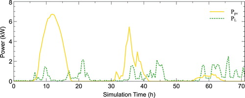
The space heating demand data is calculated for a typical one-family dwelling with 2 storeys, 150 m${}^2$ living area and a saddle roof. The building is located in Aachen, Germany, and has a building construction that complies with the German energy savings ordinance from 1984 (Constantin, Streblow, and Müller 2014). Specifically, the model considers thermal mass by modelling each of the nine rooms of the two-storey building separately. Thereby, each wall, ceiling and ground floor are composed of multiple layers that each have a different thermal capacitance and resistance. The thermal capacitances of windows and doors are not considered in this model, however, the capacitance of these elements is negligible compared to the other building elements. Furthermore, the model accounts for a quite detailed set point management including night setback. During operation, the set point temperature is guaranteed by a standard P-controller .³

The electrical consumption profile for a 4-person household (where hot water is not generated electrically) living in a one-family dwelling is based on Richardson et al. (2010), but with total consumption of 4000 kWh/a, which represents a typical consumption for such a household in 2017.⁴ The domestic hot water consumption is based on the occupancy profile used for determining the electrical demand (Richardson et al. 2010). Likewise, the hourly space heating profiles are computed with the freely available building simulation library Aixlib (Müller et al. 2016). PV output is determined for 21 modules, which corresponds to 7.6 kW peak PV output. The implemented PV model is based on Dubey, Sarvaiya, and Seshadri (2013). Weather data is obtained from the German Weather Service at 10-minute resolution for Aachen (Deutscher Wetterdienst 2017). It is assumed that the PV modules are facing south and have a pitch angle of 30${}^{\circ }$.

The results using the aforementioned parameters are shown in Tables 5, 6, and 7, where the final cost and error are computed using a detailed simulation of the system using the Aixlib library. Table 5 shows the results for all mixed integer linear programming (MILP) models, Table 6 shows the results for all mixed integer nonlinear programming (MINLP) models, and Table 7 shows the results for all nonlinear programming (NLP) models. Each of these problems are non-convex and generally classified as NP-complete. The difference lies in the solvers which are available for each, and the curvature of each problem. The NLPs are solved with IPOPT (Wächter and Biegler 2005), and the mixed-integer problems are solved with Bonmin (Bonami et al. 2008), which itself uses IPOPT to solve its continuous subproblems.

Table 5. Model comparison part 1: MILP models.

Model #	Grid connection	Heat pump dynamics	TS dynamics	γ	Run-time (s)	Final cost ($)	DHW error	SH error
1	Equation (2(2) $\begin{array}{rl}0\le P_G^{+}(t)& \le (1-z(t)){\overline{P}}_G\\ z(t){\underset{\_}{P}}_G\le P_G^{-}(t)& \le 0\\ \mathrm{where}z(t)& \in \{0,1\}\end{array}$(2) )	Equation (4(4) $\begin{array}{rl}& y_{dhw}(t)\in \{0,1\},\mathrm{\forall }t\end{array}$(4) )	Equation (7(7) $\begin{array}{rl}& \rho Vc(X(t+1)-X(t))/{\mathrm{\Delta }}_t\\ & =-m(t)(T_1-T_R(t))/c(T_{ts}-T_R(t))\\ & +((Q_{eh}(t)+Q_{hp}(t)\\ & -UA(T_1+T_2-2T_R(t))\\ & -U\pi dh(T_1-T_R(t)))/(T_{ts}-T_R(t)).\end{array}$(7) )	0	236.21	1.97	0.10	0.10
2	Equation (2(2) $\begin{array}{rl}0\le P_G^{+}(t)& \le (1-z(t)){\overline{P}}_G\\ z(t){\underset{\_}{P}}_G\le P_G^{-}(t)& \le 0\\ \mathrm{where}z(t)& \in \{0,1\}\end{array}$(2) )	Equation (4(4) $\begin{array}{rl}& y_{dhw}(t)\in \{0,1\},\mathrm{\forall }t\end{array}$(4) )	Equation (7(7) $\begin{array}{rl}& \rho Vc(X(t+1)-X(t))/{\mathrm{\Delta }}_t\\ & =-m(t)(T_1-T_R(t))/c(T_{ts}-T_R(t))\\ & +((Q_{eh}(t)+Q_{hp}(t)\\ & -UA(T_1+T_2-2T_R(t))\\ & -U\pi dh(T_1-T_R(t)))/(T_{ts}-T_R(t)).\end{array}$(7) )	0.1	239.36	2.34	0.14	0.09
3	Equation (2(2) $\begin{array}{rl}0\le P_G^{+}(t)& \le (1-z(t)){\overline{P}}_G\\ z(t){\underset{\_}{P}}_G\le P_G^{-}(t)& \le 0\\ \mathrm{where}z(t)& \in \{0,1\}\end{array}$(2) )	Equation (4(4) $\begin{array}{rl}& y_{dhw}(t)\in \{0,1\},\mathrm{\forall }t\end{array}$(4) )	Equation (7(7) $\begin{array}{rl}& \rho Vc(X(t+1)-X(t))/{\mathrm{\Delta }}_t\\ & =-m(t)(T_1-T_R(t))/c(T_{ts}-T_R(t))\\ & +((Q_{eh}(t)+Q_{hp}(t)\\ & -UA(T_1+T_2-2T_R(t))\\ & -U\pi dh(T_1-T_R(t)))/(T_{ts}-T_R(t)).\end{array}$(7) )	0.5	247.23	2.05	0.11	0.09
4	Equation (2(2) $\begin{array}{rl}0\le P_G^{+}(t)& \le (1-z(t)){\overline{P}}_G\\ z(t){\underset{\_}{P}}_G\le P_G^{-}(t)& \le 0\\ \mathrm{where}z(t)& \in \{0,1\}\end{array}$(2) )	Equation (4(4) $\begin{array}{rl}& y_{dhw}(t)\in \{0,1\},\mathrm{\forall }t\end{array}$(4) )	Equation (6(6) $\begin{array}{rl}& \rho Vc(X(t+1)-X(t))/{\mathrm{\Delta }}_t\\ & =-m(t)/c+(Q_{eh}(t)+Q_{hp}(t)\\ & -UA(T_1+T_3-2T_R(t))\\ & -U\pi dh(T_2-T_R(t)))/(T_{ts}-T_3).\end{array}$(6) )	0	225.02	2.11	0.50	0.13
5	Equation (2(2) $\begin{array}{rl}0\le P_G^{+}(t)& \le (1-z(t)){\overline{P}}_G\\ z(t){\underset{\_}{P}}_G\le P_G^{-}(t)& \le 0\\ \mathrm{where}z(t)& \in \{0,1\}\end{array}$(2) )	Equation (4(4) $\begin{array}{rl}& y_{dhw}(t)\in \{0,1\},\mathrm{\forall }t\end{array}$(4) )	Equation (6(6) $\begin{array}{rl}& \rho Vc(X(t+1)-X(t))/{\mathrm{\Delta }}_t\\ & =-m(t)/c+(Q_{eh}(t)+Q_{hp}(t)\\ & -UA(T_1+T_3-2T_R(t))\\ & -U\pi dh(T_2-T_R(t)))/(T_{ts}-T_3).\end{array}$(6) )	0.1	222.56	2.33	0.48	0.06
6	Equation (2(2) $\begin{array}{rl}0\le P_G^{+}(t)& \le (1-z(t)){\overline{P}}_G\\ z(t){\underset{\_}{P}}_G\le P_G^{-}(t)& \le 0\\ \mathrm{where}z(t)& \in \{0,1\}\end{array}$(2) )	Equation (4(4) $\begin{array}{rl}& y_{dhw}(t)\in \{0,1\},\mathrm{\forall }t\end{array}$(4) )	Equation (6(6) $\begin{array}{rl}& \rho Vc(X(t+1)-X(t))/{\mathrm{\Delta }}_t\\ & =-m(t)/c+(Q_{eh}(t)+Q_{hp}(t)\\ & -UA(T_1+T_3-2T_R(t))\\ & -U\pi dh(T_2-T_R(t)))/(T_{ts}-T_3).\end{array}$(6) )	0.5	263.23	2.24	0.37	0.20
7	Equation (2(2) $\begin{array}{rl}0\le P_G^{+}(t)& \le (1-z(t)){\overline{P}}_G\\ z(t){\underset{\_}{P}}_G\le P_G^{-}(t)& \le 0\\ \mathrm{where}z(t)& \in \{0,1\}\end{array}$(2) )	Equation (5(5) $\begin{array}{rl}& 0\le y_{dhw}(t)\le 1,\mathrm{\forall }t\end{array}$(5) )	Equation (7(7) $\begin{array}{rl}& \rho Vc(X(t+1)-X(t))/{\mathrm{\Delta }}_t\\ & =-m(t)(T_1-T_R(t))/c(T_{ts}-T_R(t))\\ & +((Q_{eh}(t)+Q_{hp}(t)\\ & -UA(T_1+T_2-2T_R(t))\\ & -U\pi dh(T_1-T_R(t)))/(T_{ts}-T_R(t)).\end{array}$(7) )	0	4.45	1.77	0.11	0.08
8	Equation (2(2) $\begin{array}{rl}0\le P_G^{+}(t)& \le (1-z(t)){\overline{P}}_G\\ z(t){\underset{\_}{P}}_G\le P_G^{-}(t)& \le 0\\ \mathrm{where}z(t)& \in \{0,1\}\end{array}$(2) )	Equation (5(5) $\begin{array}{rl}& 0\le y_{dhw}(t)\le 1,\mathrm{\forall }t\end{array}$(5) )	Equation (7(7) $\begin{array}{rl}& \rho Vc(X(t+1)-X(t))/{\mathrm{\Delta }}_t\\ & =-m(t)(T_1-T_R(t))/c(T_{ts}-T_R(t))\\ & +((Q_{eh}(t)+Q_{hp}(t)\\ & -UA(T_1+T_2-2T_R(t))\\ & -U\pi dh(T_1-T_R(t)))/(T_{ts}-T_R(t)).\end{array}$(7) )	0.1	4.51	2.09	0.11	0.08
9	Equation (2(2) $\begin{array}{rl}0\le P_G^{+}(t)& \le (1-z(t)){\overline{P}}_G\\ z(t){\underset{\_}{P}}_G\le P_G^{-}(t)& \le 0\\ \mathrm{where}z(t)& \in \{0,1\}\end{array}$(2) )	Equation (5(5) $\begin{array}{rl}& 0\le y_{dhw}(t)\le 1,\mathrm{\forall }t\end{array}$(5) )	Equation (7(7) $\begin{array}{rl}& \rho Vc(X(t+1)-X(t))/{\mathrm{\Delta }}_t\\ & =-m(t)(T_1-T_R(t))/c(T_{ts}-T_R(t))\\ & +((Q_{eh}(t)+Q_{hp}(t)\\ & -UA(T_1+T_2-2T_R(t))\\ & -U\pi dh(T_1-T_R(t)))/(T_{ts}-T_R(t)).\end{array}$(7) )	0.5	4.51	1.73	0.21	0.10
10	Equation (2(2) $\begin{array}{rl}0\le P_G^{+}(t)& \le (1-z(t)){\overline{P}}_G\\ z(t){\underset{\_}{P}}_G\le P_G^{-}(t)& \le 0\\ \mathrm{where}z(t)& \in \{0,1\}\end{array}$(2) )	Equation (5(5) $\begin{array}{rl}& 0\le y_{dhw}(t)\le 1,\mathrm{\forall }t\end{array}$(5) )	Equation (6(6) $\begin{array}{rl}& \rho Vc(X(t+1)-X(t))/{\mathrm{\Delta }}_t\\ & =-m(t)/c+(Q_{eh}(t)+Q_{hp}(t)\\ & -UA(T_1+T_3-2T_R(t))\\ & -U\pi dh(T_2-T_R(t)))/(T_{ts}-T_3).\end{array}$(6) )	0	4.30	1.84	0.29	0.08
11	Equation (2(2) $\begin{array}{rl}0\le P_G^{+}(t)& \le (1-z(t)){\overline{P}}_G\\ z(t){\underset{\_}{P}}_G\le P_G^{-}(t)& \le 0\\ \mathrm{where}z(t)& \in \{0,1\}\end{array}$(2) )	Equation (5(5) $\begin{array}{rl}& 0\le y_{dhw}(t)\le 1,\mathrm{\forall }t\end{array}$(5) )	Equation (6(6) $\begin{array}{rl}& \rho Vc(X(t+1)-X(t))/{\mathrm{\Delta }}_t\\ & =-m(t)/c+(Q_{eh}(t)+Q_{hp}(t)\\ & -UA(T_1+T_3-2T_R(t))\\ & -U\pi dh(T_2-T_R(t)))/(T_{ts}-T_3).\end{array}$(6) )	0.1	4.32	2.27	0.27	0.08
12	Equation (2(2) $\begin{array}{rl}0\le P_G^{+}(t)& \le (1-z(t)){\overline{P}}_G\\ z(t){\underset{\_}{P}}_G\le P_G^{-}(t)& \le 0\\ \mathrm{where}z(t)& \in \{0,1\}\end{array}$(2) )	Equation (5(5) $\begin{array}{rl}& 0\le y_{dhw}(t)\le 1,\mathrm{\forall }t\end{array}$(5) )	Equation (6(6) $\begin{array}{rl}& \rho Vc(X(t+1)-X(t))/{\mathrm{\Delta }}_t\\ & =-m(t)/c+(Q_{eh}(t)+Q_{hp}(t)\\ & -UA(T_1+T_3-2T_R(t))\\ & -U\pi dh(T_2-T_R(t)))/(T_{ts}-T_3).\end{array}$(6) )	0.5	4.43	2.52	0.34	0.08

Table 6. Model comparison part 2: NLP models.

Model #	Grid connection	Heat pump dynamics	TS dynamics	γ	Run-time (s)	Final cost ($)	DHW error	SH error
13	Equation (3(3) $\begin{array}{rl}0\le P_G^{+}(t)& \le {\overline{P}}_G\\ {\underset{\_}{P}}_G\le P_G^{-}(t)& \le 0\\ ϵ\le P_G^{+}(t)P_G^{-}(t)& \le 0\\ \mathrm{for}\mathrm{some}ϵ& <0\end{array}$(3) )	Equation (5(5) $\begin{array}{rl}& 0\le y_{dhw}(t)\le 1,\mathrm{\forall }t\end{array}$(5) )	Equation (8(8) $\begin{array}{rl}& \rho Vc(T_2(t+1)-T_2(t))/{\mathrm{\Delta }}_t\\ & =m(t)/c(T_3(t)-T_2(t))\\ & +Q_{hp}(t)(T_1(t)-T_2(t))/(T_{ts}-T_3(t))\\ & -U\pi dh(T_2(t)-T_R(t))\\ & +kA(T_3(t)+T_1(t)-2T_2(t))/0.2\mathrm{h}\end{array}$(8) )	0	4.04	1.96	0.10	0.08
14	Equation (3(3) $\begin{array}{rl}0\le P_G^{+}(t)& \le {\overline{P}}_G\\ {\underset{\_}{P}}_G\le P_G^{-}(t)& \le 0\\ ϵ\le P_G^{+}(t)P_G^{-}(t)& \le 0\\ \mathrm{for}\mathrm{some}ϵ& <0\end{array}$(3) )	Equation (5(5) $\begin{array}{rl}& 0\le y_{dhw}(t)\le 1,\mathrm{\forall }t\end{array}$(5) )	Equation (8(8) $\begin{array}{rl}& \rho Vc(T_2(t+1)-T_2(t))/{\mathrm{\Delta }}_t\\ & =m(t)/c(T_3(t)-T_2(t))\\ & +Q_{hp}(t)(T_1(t)-T_2(t))/(T_{ts}-T_3(t))\\ & -U\pi dh(T_2(t)-T_R(t))\\ & +kA(T_3(t)+T_1(t)-2T_2(t))/0.2\mathrm{h}\end{array}$(8) )	0.1	4.05	1.96	0.10	0.08
15	Equation (3(3) $\begin{array}{rl}0\le P_G^{+}(t)& \le {\overline{P}}_G\\ {\underset{\_}{P}}_G\le P_G^{-}(t)& \le 0\\ ϵ\le P_G^{+}(t)P_G^{-}(t)& \le 0\\ \mathrm{for}\mathrm{some}ϵ& <0\end{array}$(3) )	Equation (5(5) $\begin{array}{rl}& 0\le y_{dhw}(t)\le 1,\mathrm{\forall }t\end{array}$(5) )	Equation (8(8) $\begin{array}{rl}& \rho Vc(T_2(t+1)-T_2(t))/{\mathrm{\Delta }}_t\\ & =m(t)/c(T_3(t)-T_2(t))\\ & +Q_{hp}(t)(T_1(t)-T_2(t))/(T_{ts}-T_3(t))\\ & -U\pi dh(T_2(t)-T_R(t))\\ & +kA(T_3(t)+T_1(t)-2T_2(t))/0.2\mathrm{h}\end{array}$(8) )	0.5	4.15	2.14	0.19	0.08
16	Equation (3(3) $\begin{array}{rl}0\le P_G^{+}(t)& \le {\overline{P}}_G\\ {\underset{\_}{P}}_G\le P_G^{-}(t)& \le 0\\ ϵ\le P_G^{+}(t)P_G^{-}(t)& \le 0\\ \mathrm{for}\mathrm{some}ϵ& <0\end{array}$(3) )	Equation (5(5) $\begin{array}{rl}& 0\le y_{dhw}(t)\le 1,\mathrm{\forall }t\end{array}$(5) )	Equation (7(7) $\begin{array}{rl}& \rho Vc(X(t+1)-X(t))/{\mathrm{\Delta }}_t\\ & =-m(t)(T_1-T_R(t))/c(T_{ts}-T_R(t))\\ & +((Q_{eh}(t)+Q_{hp}(t)\\ & -UA(T_1+T_2-2T_R(t))\\ & -U\pi dh(T_1-T_R(t)))/(T_{ts}-T_R(t)).\end{array}$(7) )	0	4.12	1.89	0.11	0.08
17	Equation (3(3) $\begin{array}{rl}0\le P_G^{+}(t)& \le {\overline{P}}_G\\ {\underset{\_}{P}}_G\le P_G^{-}(t)& \le 0\\ ϵ\le P_G^{+}(t)P_G^{-}(t)& \le 0\\ \mathrm{for}\mathrm{some}ϵ& <0\end{array}$(3) )	Equation (5(5) $\begin{array}{rl}& 0\le y_{dhw}(t)\le 1,\mathrm{\forall }t\end{array}$(5) )	Equation (7(7) $\begin{array}{rl}& \rho Vc(X(t+1)-X(t))/{\mathrm{\Delta }}_t\\ & =-m(t)(T_1-T_R(t))/c(T_{ts}-T_R(t))\\ & +((Q_{eh}(t)+Q_{hp}(t)\\ & -UA(T_1+T_2-2T_R(t))\\ & -U\pi dh(T_1-T_R(t)))/(T_{ts}-T_R(t)).\end{array}$(7) )	0.1	4.10	2.04	0.11	0.07
18	Equation (3(3) $\begin{array}{rl}0\le P_G^{+}(t)& \le {\overline{P}}_G\\ {\underset{\_}{P}}_G\le P_G^{-}(t)& \le 0\\ ϵ\le P_G^{+}(t)P_G^{-}(t)& \le 0\\ \mathrm{for}\mathrm{some}ϵ& <0\end{array}$(3) )	Equation (5(5) $\begin{array}{rl}& 0\le y_{dhw}(t)\le 1,\mathrm{\forall }t\end{array}$(5) )	Equation (7(7) $\begin{array}{rl}& \rho Vc(X(t+1)-X(t))/{\mathrm{\Delta }}_t\\ & =-m(t)(T_1-T_R(t))/c(T_{ts}-T_R(t))\\ & +((Q_{eh}(t)+Q_{hp}(t)\\ & -UA(T_1+T_2-2T_R(t))\\ & -U\pi dh(T_1-T_R(t)))/(T_{ts}-T_R(t)).\end{array}$(7) )	0.5	4.20	1.89	0.14	0.09
19	Equation (3(3) $\begin{array}{rl}0\le P_G^{+}(t)& \le {\overline{P}}_G\\ {\underset{\_}{P}}_G\le P_G^{-}(t)& \le 0\\ ϵ\le P_G^{+}(t)P_G^{-}(t)& \le 0\\ \mathrm{for}\mathrm{some}ϵ& <0\end{array}$(3) )	Equation (5(5) $\begin{array}{rl}& 0\le y_{dhw}(t)\le 1,\mathrm{\forall }t\end{array}$(5) )	Equation (6(6) $\begin{array}{rl}& \rho Vc(X(t+1)-X(t))/{\mathrm{\Delta }}_t\\ & =-m(t)/c+(Q_{eh}(t)+Q_{hp}(t)\\ & -UA(T_1+T_3-2T_R(t))\\ & -U\pi dh(T_2-T_R(t)))/(T_{ts}-T_3).\end{array}$(6) )	0	3.81	1.77	0.27	0.08
20	Equation (3(3) $\begin{array}{rl}0\le P_G^{+}(t)& \le {\overline{P}}_G\\ {\underset{\_}{P}}_G\le P_G^{-}(t)& \le 0\\ ϵ\le P_G^{+}(t)P_G^{-}(t)& \le 0\\ \mathrm{for}\mathrm{some}ϵ& <0\end{array}$(3) )	Equation (5(5) $\begin{array}{rl}& 0\le y_{dhw}(t)\le 1,\mathrm{\forall }t\end{array}$(5) )	Equation (6(6) $\begin{array}{rl}& \rho Vc(X(t+1)-X(t))/{\mathrm{\Delta }}_t\\ & =-m(t)/c+(Q_{eh}(t)+Q_{hp}(t)\\ & -UA(T_1+T_3-2T_R(t))\\ & -U\pi dh(T_2-T_R(t)))/(T_{ts}-T_3).\end{array}$(6) )	0.1	3.88	2.18	0.29	0.08
21	Equation (3(3) $\begin{array}{rl}0\le P_G^{+}(t)& \le {\overline{P}}_G\\ {\underset{\_}{P}}_G\le P_G^{-}(t)& \le 0\\ ϵ\le P_G^{+}(t)P_G^{-}(t)& \le 0\\ \mathrm{for}\mathrm{some}ϵ& <0\end{array}$(3) )	Equation (5(5) $\begin{array}{rl}& 0\le y_{dhw}(t)\le 1,\mathrm{\forall }t\end{array}$(5) )	Equation (6(6) $\begin{array}{rl}& \rho Vc(X(t+1)-X(t))/{\mathrm{\Delta }}_t\\ & =-m(t)/c+(Q_{eh}(t)+Q_{hp}(t)\\ & -UA(T_1+T_3-2T_R(t))\\ & -U\pi dh(T_2-T_R(t)))/(T_{ts}-T_3).\end{array}$(6) )	0.5	3.92	2.55	0.30	0.07

Table 7. Model comparison part 3: MINLP models.

Model #	Grid connection	Heat pump dynamics	TS dynamics	γ	Run-time (s)	Final cost ($)	DHW error	SH error
22	Equation (2(2) $\begin{array}{rl}0\le P_G^{+}(t)& \le (1-z(t)){\overline{P}}_G\\ z(t){\underset{\_}{P}}_G\le P_G^{-}(t)& \le 0\\ \mathrm{where}z(t)& \in \{0,1\}\end{array}$(2) )	Equation (4(4) $\begin{array}{rl}& y_{dhw}(t)\in \{0,1\},\mathrm{\forall }t\end{array}$(4) )	Equation (8(8) $\begin{array}{rl}& \rho Vc(T_2(t+1)-T_2(t))/{\mathrm{\Delta }}_t\\ & =m(t)/c(T_3(t)-T_2(t))\\ & +Q_{hp}(t)(T_1(t)-T_2(t))/(T_{ts}-T_3(t))\\ & -U\pi dh(T_2(t)-T_R(t))\\ & +kA(T_3(t)+T_1(t)-2T_2(t))/0.2\mathrm{h}\end{array}$(8) )	0	285.01	2.71	0.23	0.08
23	Equation (2(2) $\begin{array}{rl}0\le P_G^{+}(t)& \le (1-z(t)){\overline{P}}_G\\ z(t){\underset{\_}{P}}_G\le P_G^{-}(t)& \le 0\\ \mathrm{where}z(t)& \in \{0,1\}\end{array}$(2) )	Equation (4(4) $\begin{array}{rl}& y_{dhw}(t)\in \{0,1\},\mathrm{\forall }t\end{array}$(4) )	Equation (8(8) $\begin{array}{rl}& \rho Vc(T_2(t+1)-T_2(t))/{\mathrm{\Delta }}_t\\ & =m(t)/c(T_3(t)-T_2(t))\\ & +Q_{hp}(t)(T_1(t)-T_2(t))/(T_{ts}-T_3(t))\\ & -U\pi dh(T_2(t)-T_R(t))\\ & +kA(T_3(t)+T_1(t)-2T_2(t))/0.2\mathrm{h}\end{array}$(8) )	0.1	266.85	2.68	0.35	0.07
24	Equation (2(2) $\begin{array}{rl}0\le P_G^{+}(t)& \le (1-z(t)){\overline{P}}_G\\ z(t){\underset{\_}{P}}_G\le P_G^{-}(t)& \le 0\\ \mathrm{where}z(t)& \in \{0,1\}\end{array}$(2) )	Equation (4(4) $\begin{array}{rl}& y_{dhw}(t)\in \{0,1\},\mathrm{\forall }t\end{array}$(4) )	Equation (8(8) $\begin{array}{rl}& \rho Vc(T_2(t+1)-T_2(t))/{\mathrm{\Delta }}_t\\ & =m(t)/c(T_3(t)-T_2(t))\\ & +Q_{hp}(t)(T_1(t)-T_2(t))/(T_{ts}-T_3(t))\\ & -U\pi dh(T_2(t)-T_R(t))\\ & +kA(T_3(t)+T_1(t)-2T_2(t))/0.2\mathrm{h}\end{array}$(8) )	$0.5$	268.09	2.41	0.44	0.08
25	Equation (2(2) $\begin{array}{rl}0\le P_G^{+}(t)& \le (1-z(t)){\overline{P}}_G\\ z(t){\underset{\_}{P}}_G\le P_G^{-}(t)& \le 0\\ \mathrm{where}z(t)& \in \{0,1\}\end{array}$(2) )	Equation (5(5) $\begin{array}{rl}& 0\le y_{dhw}(t)\le 1,\mathrm{\forall }t\end{array}$(5) )	Equation (8(8) $\begin{array}{rl}& \rho Vc(T_2(t+1)-T_2(t))/{\mathrm{\Delta }}_t\\ & =m(t)/c(T_3(t)-T_2(t))\\ & +Q_{hp}(t)(T_1(t)-T_2(t))/(T_{ts}-T_3(t))\\ & -U\pi dh(T_2(t)-T_R(t))\\ & +kA(T_3(t)+T_1(t)-2T_2(t))/0.2\mathrm{h}\end{array}$(8) )	0	4.58	1.91	0.10	0.08
26	Equation (2(2) $\begin{array}{rl}0\le P_G^{+}(t)& \le (1-z(t)){\overline{P}}_G\\ z(t){\underset{\_}{P}}_G\le P_G^{-}(t)& \le 0\\ \mathrm{where}z(t)& \in \{0,1\}\end{array}$(2) )	Equation (5(5) $\begin{array}{rl}& 0\le y_{dhw}(t)\le 1,\mathrm{\forall }t\end{array}$(5) )	Equation (8(8) $\begin{array}{rl}& \rho Vc(T_2(t+1)-T_2(t))/{\mathrm{\Delta }}_t\\ & =m(t)/c(T_3(t)-T_2(t))\\ & +Q_{hp}(t)(T_1(t)-T_2(t))/(T_{ts}-T_3(t))\\ & -U\pi dh(T_2(t)-T_R(t))\\ & +kA(T_3(t)+T_1(t)-2T_2(t))/0.2\mathrm{h}\end{array}$(8) )	0.1	4.63	2.08	0.10	0.08
27	Equation (2(2) $\begin{array}{rl}0\le P_G^{+}(t)& \le (1-z(t)){\overline{P}}_G\\ z(t){\underset{\_}{P}}_G\le P_G^{-}(t)& \le 0\\ \mathrm{where}z(t)& \in \{0,1\}\end{array}$(2) )	Equation (5(5) $\begin{array}{rl}& 0\le y_{dhw}(t)\le 1,\mathrm{\forall }t\end{array}$(5) )	Equation (8(8) $\begin{array}{rl}& \rho Vc(T_2(t+1)-T_2(t))/{\mathrm{\Delta }}_t\\ & =m(t)/c(T_3(t)-T_2(t))\\ & +Q_{hp}(t)(T_1(t)-T_2(t))/(T_{ts}-T_3(t))\\ & -U\pi dh(T_2(t)-T_R(t))\\ & +kA(T_3(t)+T_1(t)-2T_2(t))/0.2\mathrm{h}\end{array}$(8) )	0.5	4.64	1.78	0.25	0.09
28	Equation (3(3) $\begin{array}{rl}0\le P_G^{+}(t)& \le {\overline{P}}_G\\ {\underset{\_}{P}}_G\le P_G^{-}(t)& \le 0\\ ϵ\le P_G^{+}(t)P_G^{-}(t)& \le 0\\ \mathrm{for}\mathrm{some}ϵ& <0\end{array}$(3) )	Equation (4(4) $\begin{array}{rl}& y_{dhw}(t)\in \{0,1\},\mathrm{\forall }t\end{array}$(4) )	Equation (8(8) $\begin{array}{rl}& \rho Vc(T_2(t+1)-T_2(t))/{\mathrm{\Delta }}_t\\ & =m(t)/c(T_3(t)-T_2(t))\\ & +Q_{hp}(t)(T_1(t)-T_2(t))/(T_{ts}-T_3(t))\\ & -U\pi dh(T_2(t)-T_R(t))\\ & +kA(T_3(t)+T_1(t)-2T_2(t))/0.2\mathrm{h}\end{array}$(8) )	0	274.04	2.75	0.20	0.11
29	Equation (3(3) $\begin{array}{rl}0\le P_G^{+}(t)& \le {\overline{P}}_G\\ {\underset{\_}{P}}_G\le P_G^{-}(t)& \le 0\\ ϵ\le P_G^{+}(t)P_G^{-}(t)& \le 0\\ \mathrm{for}\mathrm{some}ϵ& <0\end{array}$(3) )	Equation (4(4) $\begin{array}{rl}& y_{dhw}(t)\in \{0,1\},\mathrm{\forall }t\end{array}$(4) )	Equation (8(8) $\begin{array}{rl}& \rho Vc(T_2(t+1)-T_2(t))/{\mathrm{\Delta }}_t\\ & =m(t)/c(T_3(t)-T_2(t))\\ & +Q_{hp}(t)(T_1(t)-T_2(t))/(T_{ts}-T_3(t))\\ & -U\pi dh(T_2(t)-T_R(t))\\ & +kA(T_3(t)+T_1(t)-2T_2(t))/0.2\mathrm{h}\end{array}$(8) )	0.1	268.44	2.77	0.23	0.07
30	Equation (3(3) $\begin{array}{rl}0\le P_G^{+}(t)& \le {\overline{P}}_G\\ {\underset{\_}{P}}_G\le P_G^{-}(t)& \le 0\\ ϵ\le P_G^{+}(t)P_G^{-}(t)& \le 0\\ \mathrm{for}\mathrm{some}ϵ& <0\end{array}$(3) )	Equation (4(4) $\begin{array}{rl}& y_{dhw}(t)\in \{0,1\},\mathrm{\forall }t\end{array}$(4) )	Equation (8(8) $\begin{array}{rl}& \rho Vc(T_2(t+1)-T_2(t))/{\mathrm{\Delta }}_t\\ & =m(t)/c(T_3(t)-T_2(t))\\ & +Q_{hp}(t)(T_1(t)-T_2(t))/(T_{ts}-T_3(t))\\ & -U\pi dh(T_2(t)-T_R(t))\\ & +kA(T_3(t)+T_1(t)-2T_2(t))/0.2\mathrm{h}\end{array}$(8) )	0.5	259.16	2.25	0.38	0.09
31	Equation (3(3) $\begin{array}{rl}0\le P_G^{+}(t)& \le {\overline{P}}_G\\ {\underset{\_}{P}}_G\le P_G^{-}(t)& \le 0\\ ϵ\le P_G^{+}(t)P_G^{-}(t)& \le 0\\ \mathrm{for}\mathrm{some}ϵ& <0\end{array}$(3) )	Equation (4(4) $\begin{array}{rl}& y_{dhw}(t)\in \{0,1\},\mathrm{\forall }t\end{array}$(4) )	Equation (7(7) $\begin{array}{rl}& \rho Vc(X(t+1)-X(t))/{\mathrm{\Delta }}_t\\ & =-m(t)(T_1-T_R(t))/c(T_{ts}-T_R(t))\\ & +((Q_{eh}(t)+Q_{hp}(t)\\ & -UA(T_1+T_2-2T_R(t))\\ & -U\pi dh(T_1-T_R(t)))/(T_{ts}-T_R(t)).\end{array}$(7) )	0	237.73	2.14	0.11	0.11
32	Equation (3(3) $\begin{array}{rl}0\le P_G^{+}(t)& \le {\overline{P}}_G\\ {\underset{\_}{P}}_G\le P_G^{-}(t)& \le 0\\ ϵ\le P_G^{+}(t)P_G^{-}(t)& \le 0\\ \mathrm{for}\mathrm{some}ϵ& <0\end{array}$(3) )	Equation (4(4) $\begin{array}{rl}& y_{dhw}(t)\in \{0,1\},\mathrm{\forall }t\end{array}$(4) )	Equation (7(7) $\begin{array}{rl}& \rho Vc(X(t+1)-X(t))/{\mathrm{\Delta }}_t\\ & =-m(t)(T_1-T_R(t))/c(T_{ts}-T_R(t))\\ & +((Q_{eh}(t)+Q_{hp}(t)\\ & -UA(T_1+T_2-2T_R(t))\\ & -U\pi dh(T_1-T_R(t)))/(T_{ts}-T_R(t)).\end{array}$(7) )	0.1	255.07	2.48	0.14	0.12
33	Equation (3(3) $\begin{array}{rl}0\le P_G^{+}(t)& \le {\overline{P}}_G\\ {\underset{\_}{P}}_G\le P_G^{-}(t)& \le 0\\ ϵ\le P_G^{+}(t)P_G^{-}(t)& \le 0\\ \mathrm{for}\mathrm{some}ϵ& <0\end{array}$(3) )	Equation (4(4) $\begin{array}{rl}& y_{dhw}(t)\in \{0,1\},\mathrm{\forall }t\end{array}$(4) )	Equation (7(7) $\begin{array}{rl}& \rho Vc(X(t+1)-X(t))/{\mathrm{\Delta }}_t\\ & =-m(t)(T_1-T_R(t))/c(T_{ts}-T_R(t))\\ & +((Q_{eh}(t)+Q_{hp}(t)\\ & -UA(T_1+T_2-2T_R(t))\\ & -U\pi dh(T_1-T_R(t)))/(T_{ts}-T_R(t)).\end{array}$(7) )	0.5	197.81	2.54	0.06	0.12
34	Equation (3(3) $\begin{array}{rl}0\le P_G^{+}(t)& \le {\overline{P}}_G\\ {\underset{\_}{P}}_G\le P_G^{-}(t)& \le 0\\ ϵ\le P_G^{+}(t)P_G^{-}(t)& \le 0\\ \mathrm{for}\mathrm{some}ϵ& <0\end{array}$(3) )	Equation (4(4) $\begin{array}{rl}& y_{dhw}(t)\in \{0,1\},\mathrm{\forall }t\end{array}$(4) )	Equation (6(6) $\begin{array}{rl}& \rho Vc(X(t+1)-X(t))/{\mathrm{\Delta }}_t\\ & =-m(t)/c+(Q_{eh}(t)+Q_{hp}(t)\\ & -UA(T_1+T_3-2T_R(t))\\ & -U\pi dh(T_2-T_R(t)))/(T_{ts}-T_3).\end{array}$(6) )	0	235.54	2.35	0.42	0.11
35	Equation (3(3) $\begin{array}{rl}0\le P_G^{+}(t)& \le {\overline{P}}_G\\ {\underset{\_}{P}}_G\le P_G^{-}(t)& \le 0\\ ϵ\le P_G^{+}(t)P_G^{-}(t)& \le 0\\ \mathrm{for}\mathrm{some}ϵ& <0\end{array}$(3) )	Equation (4(4) $\begin{array}{rl}& y_{dhw}(t)\in \{0,1\},\mathrm{\forall }t\end{array}$(4) )	Equation (6(6) $\begin{array}{rl}& \rho Vc(X(t+1)-X(t))/{\mathrm{\Delta }}_t\\ & =-m(t)/c+(Q_{eh}(t)+Q_{hp}(t)\\ & -UA(T_1+T_3-2T_R(t))\\ & -U\pi dh(T_2-T_R(t)))/(T_{ts}-T_3).\end{array}$(6) )	0.1	199.13	1.87	0.47	0.08
36	Equation (3(3) $\begin{array}{rl}0\le P_G^{+}(t)& \le {\overline{P}}_G\\ {\underset{\_}{P}}_G\le P_G^{-}(t)& \le 0\\ ϵ\le P_G^{+}(t)P_G^{-}(t)& \le 0\\ \mathrm{for}\mathrm{some}ϵ& <0\end{array}$(3) )	Equation (4(4) $\begin{array}{rl}& y_{dhw}(t)\in \{0,1\},\mathrm{\forall }t\end{array}$(4) )	Equation (6(6) $\begin{array}{rl}& \rho Vc(X(t+1)-X(t))/{\mathrm{\Delta }}_t\\ & =-m(t)/c+(Q_{eh}(t)+Q_{hp}(t)\\ & -UA(T_1+T_3-2T_R(t))\\ & -U\pi dh(T_2-T_R(t)))/(T_{ts}-T_3).\end{array}$(6) )	0.5	213.08	3.10	0.39	0.20

The final cost for each model is based on the actual power usage as calculated in the Aixlib simulation model. The DHW and SH errors are taken as a sum of squares of the difference between the energy states of the thermal storage model and the simulation model over the entire time horizon H. (12) $\begin{array}{r}Error=\sum _{t=1}^H{(X(t)-X_{sim}(t))}^2\end{array}$(12) where $X(t)$ is what is predicted for the next time step based on the relevant thermal storage model from Section 2, and $X_{sim}(t)$ is what actually occurred. This is computed via $X_{sim}(t)=V_{usable}(t)/V$, where $V_{usable}$ is the volume of water above $T_{sh}$ or $T_{dhw}$, depending on the thermal storage tank in question.

The errors for the domestic how water tank are on average 2.53 times higher than the errors for the space heating storage tank. This finding is also supported by Figure 4. In these figures, the dynamics of the space heating tank are more accurately modelled than the smaller domestic hot water tank. However, both models are still fairly accurate in the short term, and thus don't result in particularly large errors overall.

3.1. Sensitivity analysis

To assess the extent to which the results of Section 3 are dependent on the fixed parameters described in Section 2, the following problem variants are tested:

• Battery capacity increased by 20%

• Battery capacity decreased by 20%

• Thermal storage capacity increased by 20%

• Thermal storage capacity decreased by 20%

• Heating and electrical loads increased by 20%

• Heating and electrical loads decreased by 20%

The maximum and minimum results from these tests are shown in Tables 8, 9, and 10. The model numbers shown in these tables correspond with those shown in Tables 5, 6, and 7.

Table 8. Model comparison part 1: MILP models.

	Runtime(s)		Final cost($)		DHW error		SH error
Model #	Min.	Max.	Min.	Max.	Min.	Max.	Min.	Max.
1	225.07	281.16	−0.40	4.87	0.06	0.20	0.09	0.15
2	210.70	301.81	−0.24	5.00	0.06	0.16	0.08	0.16
3	177.08	251.19	0.05	4.85	0.07	0.27	0.07	0.16
4	189.31	268.09	−0.42	4.31	0.34	0.58	0.07	0.18
5	172.77	285.01	−0.21	5.16	0.23	0.55	0.06	0.16
6	173.08	266.85	0.22	4.36	0.35	0.49	0.07	0.23
7	0.86	4.85	−0.60	2.58	0.01	0.21	0.04	0.10
8	0.87	4.69	−0.42	2.28	0.01	0.11	0.04	0.08
9	0.87	4.64	−0.68	2.42	0.01	0.21	0.04	0.10
10	2.17	4.73	−0.64	2.63	0.22	0.32	0.04	0.09
11	2.11	4.66	−0.27	2.30	0.10	0.31	0.04	0.08
12	2.07	4.63	−0.69	2.52	0.10	0.34	0.04	0.11

Table 9. Model comparison part 2: NLP models.

	Runtime (s)		Final cost ($)		DHW error		SH error
Model #	Min.	Max.	Min.	Max.	Min.	Max.	Min.	Max.
13	0.77	4.14	−0.25	2.81	0.01	0.30	0.04	0.08
14	0.78	4.17	−0.92	2.53	0.01	0.27	0.04	0.08
15	0.78	4.20	−0.52	2.74	0.01	0.29	0.04	0.20
16	0.75	4.20	−0.60	2.50	0.01	0.14	0.04	0.09
17	0.76	4.12	−0.23	2.07	0.01	0.11	0.04	0.09
18	0.76	4.16	−0.31	2.70	0.01	0.19	0.04	0.09
19	1.87	4.15	−0.51	2.52	0.19	0.31	0.04	0.08
20	1.87	4.04	−0.28	2.27	0.10	0.31	0.04	0.08
21	1.94	4.08	−0.44	3.05	0.10	0.35	0.04	0.08

Table 10. Model comparison part 3: MINLP models.

	Runtime(s)		Final cost($)		DHW error		SH error
Model #	Min.	Max.	Min.	Max.	Min.	Max.	Min.	Max.
22	223.35	292.55	−0.01	5.21	0.11	0.37	0.07	0.20
23	225.02	266.63	0.27	5.24	0.08	0.50	0.07	0.23
24	222.56	284.92	−0.38	4.82	0.08	0.55	0.06	0.13
25	0.88	4.85	−1.02	2.52	0.01	0.34	0.04	0.08
26	0.86	4.71	−0.12	2.31	0.01	0.29	0.04	0.08
27	0.88	4.75	−0.50	2.27	0.01	0.27	0.04	0.09
28	212.02	280.12	0.16	4.87	0.09	0.39	0.07	0.20
29	205.81	278.12	0.16	5.55	0.08	0.42	0.07	0.26
30	199.13	280.61	0.21	5.14	0.17	0.49	0.05	0.16
31	197.81	270.91	−0.50	4.82	0.06	0.17	0.08	0.12
32	215.73	255.82	−0.10	5.38	0.11	0.21	0.08	0.12
33	173.74	288.46	0.35	4.93	0.06	0.19	0.09	0.17
34	161.15	259.16	−0.26	5.21	0.36	0.52	0.04	0.21
35	184.55	274.04	0.22	4.66	0.20	0.56	0.05	0.11
36	170.71	268.44	−0.05	4.93	0.23	0.49	0.07	0.20

The negative cost is due to the case where load is decreased (but pv generation is unaffected) and excess generated power is sold to the grid. Interestingly, the runtime for models which include a continuous heat pump seems to be largely unaffected by the parameter changes, while there is significant deviation amongst the models which include discrete heat pump dynamics. The model error varies consistently amongst all models. Furthermore, none of the tests result in a consistent increase or decrease in model error. For example, the minimum SH tank error for Model 18 occurs in the case of increased load, while the SH tank error for Model 1 is highest in this case. Overall, there is a slight increase in DHW error in the case of increased loads, and a slight decrease for both TS tank errors in the case of decreased loads.

4. Analysis of results

The results from Section 3 are grouped into three categories: MILP, NLP and MINLP models. There are a number of interesting insights to be gleaned from Tables 5, 6, and 7. The first of which is that using a discrete heat pump model leads to runtimes that are 2 orders of magnitude longer than the same model with a continuous heat pump model. As the error for the space heating and domestic hot water tanks indicate, the continuous model does not have a sizable impact on accuracy. As shown in Section 3.1, the runtime of models which include discrete heat pump dynamics has some sensitivity with respect to the input parameters and load profiles, however, even in the best case the problem is not solved nearly as quickly as an equivalent model with continuous heat pump dynamics.

Second, penalizing the emptiness of the battery in the final time step of the optimization subproblems generally has an unpredictable effect on the overall cost of system operation. For example, both the most and least expensive models have $\gamma =0.5$. On average, a penalty term of 0 or 0.1 seemed to result in the lowest costs. This could be due in part to the specific electricity and heating demands, as this penalty can sometimes help mitigate the costs of unexpected peaks in electricity or heating demand, while leading to some suboptimality otherwise.

Third, whether or not the grid connection is modelled using mixed-integer or continuous, nonlinear dynamics did not seem to significantly affect the runtime, cost or accuracy of the modelled system. This is particularly interesting given the huge impact caused by the choice of continuous vs. discrete heat pump activation.

Overall, using thermal storages modelled with (6(6) $\begin{array}{rl}& \rho Vc(X(t+1)-X(t))/{\mathrm{\Delta }}_t\\ & =-m(t)/c+(Q_{eh}(t)+Q_{hp}(t)\\ & -UA(T_1+T_3-2T_R(t))\\ & -U\pi dh(T_2-T_R(t)))/(T_{ts}-T_3).\end{array}$(6) ) or (8(8) $\begin{array}{rl}& \rho Vc(T_2(t+1)-T_2(t))/{\mathrm{\Delta }}_t\\ & =m(t)/c(T_3(t)-T_2(t))\\ & +Q_{hp}(t)(T_1(t)-T_2(t))/(T_{ts}-T_3(t))\\ & -U\pi dh(T_2(t)-T_R(t))\\ & +kA(T_3(t)+T_1(t)-2T_2(t))/0.2\mathrm{h}\end{array}$(8) ) lead to the slightly faster runtime and also slightly higher cost. The lowest operational cost ($1.73) is achieved by using (2(2) $\begin{array}{rl}0\le P_G^{+}(t)& \le (1-z(t)){\overline{P}}_G\\ z(t){\underset{\_}{P}}_G\le P_G^{-}(t)& \le 0\\ \mathrm{where}z(t)& \in \{0,1\}\end{array}$(2) ) as the grid connection, (5(5) $\begin{array}{rl}& 0\le y_{dhw}(t)\le 1,\mathrm{\forall }t\end{array}$(5) ) for the heat pump and (7(7) $\begin{array}{rl}& \rho Vc(X(t+1)-X(t))/{\mathrm{\Delta }}_t\\ & =-m(t)(T_1-T_R(t))/c(T_{ts}-T_R(t))\\ & +((Q_{eh}(t)+Q_{hp}(t)\\ & -UA(T_1+T_2-2T_R(t))\\ & -U\pi dh(T_1-T_R(t)))/(T_{ts}-T_R(t)).\end{array}$(7) ) for the thermal storage model. Doing so also results in one of the slowest runtime amongst the models with continuous heat pumps (4.51 s). However, as the scale of the problem is in the order of hours and days, the difference between runtimes is quite trivial but the difference in cost is much more significant.

The solution trajectories output by the models can also offer some insight into the effects of each modelling choice. To this end, the results for the most and least expensive models from Section 3 are shown in Figures 6 and 7.

Figure 6. Thermal storage trajectories for the most and least expensive models of Section 4. $X_{dhw}$ denotes the proportion of usable water in the domestic hot water tank and $X_{sh}$ is the proportion of usable water in the space heating tank.

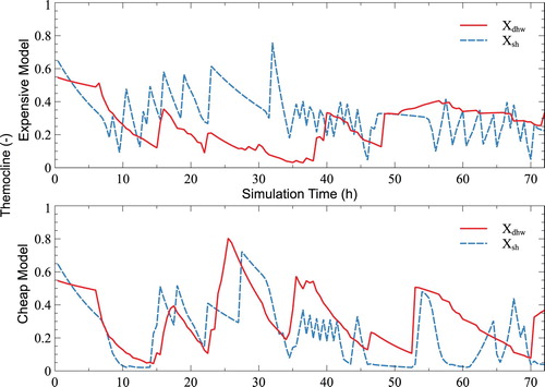
Figure 7. Solution trajectories for the most and least expensive models of Section 4.

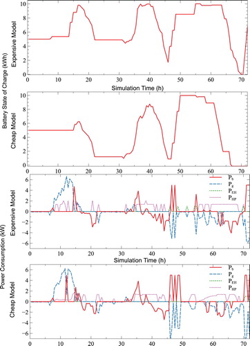
Despite the fact that both models use $\gamma =0.5$, the final state of charge for the batteries is quite different. The more expensive model has a last minute charging of the battery, which increases costs, while the least expensive ends with the battery completely depleted. Another significant factor in the cost difference is the fact that the more expensive case uses a discrete heat pump model and thus must rely on the electric heater at times. As can be observed in Figure 7, the heat pump usage is the biggest difference between both models. The least expensive case has a continuous heat pump model and thus can charge the thermal storage tanks without ever relying on the inefficient electric heater. An implementation of the continuous heat pump solution could lead to chattering behaviour as it is rapidly switched on and off to only provide limited heating. This could lead to hidden costs in maintenance which are not accounted for in the presented results.

5. Conclusion

In this paper, multiple linear and nonlinear mixed-integer problem formulations for the cost-optimal control of a multi-model home energy system are compared. Several models for each component of the combined battery, heat pump and thermal storage system are given and compared within an MPC framework.

Overall, for the given inputs, the continuous heat pump model leads to faster computing times without significantly affecting the model accuracy. The continuous heat pump is also shown to be better able to handle increased loads compared to the discrete case. However, as mentioned, there may be additional difficulties involved with implementing and using the solution to such a model. The linear thermocline-based thermal storage model yields the most cost-effective model on average while staying within reasonable runtime limits. The grid connection can be freely modelled as either a mixed-integer linear or continuous, non-convex equality constraint without loss of accuracy or speed. This choice will likely depend more on the algorithmic limitations of the user. Finally, some small penalty for the emptiness of the battery at the end of the scheduling horizon can be beneficial, although not in every case. The lowest-cost model includes a mixed-integer grid connection, continuous heat pump dynamics, a linear thermocline-based thermal storage model and a large penalty on battery emptiness at the end of the time horizon.

Future works will be conducted in multiple facets. From an optimization point of view, future studies will seek to quantify and develop heuristics for choosing the penalty for storage emptiness at the end of the scheduling horizon depending on forecast data. Regarding application, future works will also include an examination of other scenarios, such as industrial settings or atypical weather. Furthermore, future work will attempt to solve the stochastic version of the BATSS problem with chance constraints and/or flexible loads.

Furthermore, while the focus of the paper is on the modelling of heat pumps, thermal storages, and batteries, it would also be interesting to take temperature variations and room comfort into account. This could take the form of specific building topology or additional objective function terms.

6. Nomenclature

6.1. Control variables

$P_G^{+}(t)$	=	power fed to main grid at time t.
$P_G^{-}(t)$	=	power drawn from main grid at time t.
$z(t)$	=	indicator variable for power flow direction at the grid connection at time t.
$y_{dhw}(t)$	=	indicator variable for heat pump to warm the domestic hot water tank at time t.
$y_{sh}(t)$	=	indicator variable for heat pump to warm the space heating tank at time t.
$P_{bat}^{+}(t)$	=	power sent to battery at time t.
$P_{bat}^{-}(t)$	=	power drawn from battery at time t.
$z_{bat}(t)$	=	indicator variable for power flow direction at the battery at time t.
$P_{eh\to dhw}(t)$	=	power used by electric heater in domestic hot water tank at time t.
$P_{eh\to sh}(t)$	=	power used by electric heater in space heating tank at time t.

6.2. State variables

$P_{hp}(t)$	=	power used by heat pump at time t.
$Q_{hp}(t)$	=	heat output of heat pump at time t.
$X(t)$	=	thermal storage tank thermocline at time t.
$T_1(t)$	=	temperature at the bottom of the thermal storage tank at time t.
$T_2(t)$	=	temperature in the middle of the thermal storage tank at time t.
$T_3(t)$	=	temperature at the top of the thermal storage tank at time t.
$E(t)$	=	state of charge of the battery at time t.

Disclosure statement

No potential conflict of interest was reported by the author(s).

Notes

1 Regulations typically require domestic hot water to be heated to around 60 ${}^{\circ }$C for health reasons while space heating requires much less heat, at around 35 ${}^{\circ }$C for modern underfloor heating systems.

2 Future work will attempt to solve the stochastic version of the BATSS problem with chance constraints and/or flexible loads.

3 The exact data for each of the components of this model can be found at https://github.com/RWTH-EBC/AixLib/blob/development/AixLib/ThermalZones/HighOrder/Examples/OFDHeatLoad.mo

4 For the full report in German: https://www.stromspiegel.de/fileadmin/ssi/stromspiegel/Broschuere/Stromspiegel_2017_web.pdf.

References

- Setlhaolo, D., S. Sichilalu, and J. Zhang. 2017. “Residential Load Management in An Energy Hub with Heat Pump Water Heater.” Applied Energy 208: 551–560. doi: 10.1016/j.apenergy.2017.09.099
- Appino, R., A. Ordiano, R. Mikut, T. Faulwasser, and V. Hagenmeyer. 2018. “On the Use of Probabilistic Forecasts in Scheduling of Renewable Energy Sources Coupled to Storages.” Applied Energy 210: 1207–1218. doi: 10.1016/j.apenergy.2017.08.133
- Kwon, W., A. Bruckstein, and T. Kailath. 1983. “Stabilizing State Feedback Design Via the Moving Horizon Method.” International Journal of Control 37 (3): 631–643. doi: 10.1080/00207178308932998
- Mayne, D., J. Rawlings, C. Rao, and P. Scokaert. 2000. “Constrained Model Predictive Control: Stability and Optimality.” Automatica 36 (6): 789–814. doi: 10.1016/S0005-1098(99)00214-9
- Qin, S., and T. Badgwell. 2003. “A Survey of Industrial Model Predictive Control Technology.” Control Engineering Practice 11 (7): 733–764. doi: 10.1016/S0967-0661(02)00186-7
- Garcia, C., D. Prett, and M. Morari. 1989. “Model Predictive Control: Theory and Practicea Survey.” Automatica 25 (3): 335–348. doi: 10.1016/0005-1098(89)90002-2
- Arnold, M., and G. Andersson. 2011. “Model Predictive Control for Energy Storage Including Uncertain Forecasts.” Power Systems Computation Conference 23: 24–29.
- Geyer, T.. 2009. “Generalized Model Predictive Direct Torque Control: Long Prediction Horizons and Minimization of Switching Losses,” in Proceedings of the 48h IEEE Conference on Decision and Control (CDC) held jointly with 2009 28th Chinese Control Conference, 6799–6804. Shanghai: IEEE.
- Maasoumy, M., M. Razmara, M. Shahbakhti, and A. Vincentelli. 2014. “Handling Model Uncertainty in Model Predictive Control for Energy Efficient Buildings.” Energy and Buildings 77: 377–392. doi: 10.1016/j.enbuild.2014.03.057
- Oliveski, R., A. Krenzinger, and H. Vielmo. 2003. “Comparison Between Models for the Simulation of Hot Water Storage Tanks.” Solar Energy 75 (2): 121–134. doi: 10.1016/j.solener.2003.07.009
- Collazos, A., F. Maréchal, and C. Gähler. 2009. “Predictive Optimal Management Method for the Control of Polygeneration Systems.” Computers & Chemical Engineering 33 (10): 1584–1592. doi: 10.1016/j.compchemeng.2009.05.009
- Ashouri, A., S. Fux, M. Benz, and L. Guzzella. 2013. “Optimal Design and Operation of Building Services Using Mixed-Integer Linear Programming Techniques.” Energy 59:365–376. doi: 10.1016/j.energy.2013.06.053
- Wakui, T., and R. Yokoyama. 2014. “Optimal Structural Design of Residential Cogeneration Systems in Consideration of Their Operating Restrictions.” Energy 64: 719–733. doi: 10.1016/j.energy.2013.10.002
- D'Ettorre, F., P. Conti, E. Schito, and D. Testi. 2019. “Model Predictive Control of a Hybrid Heat Pump System and Impact of the Prediction Horizon on Cost-Saving Potential and Optimal Storage Capacity.” Applied Thermal Engineering 148 (5): 524–535. doi: 10.1016/j.applthermaleng.2018.11.063
- Fazlollahi, S., G. Becker, and F. Marchal. 2014. “Multi-Objectives, Multi-Period Optimization of District Energy Systems: Iidaily Thermal Storage.” Computers & Chemical Engineering 71: 648–662. doi: 10.1016/j.compchemeng.2013.10.016
- Steen, D., M. Stadler, G. Cardoso, M. Groissböck, N. DeForest, and C. Marnay. 2015. “Modeling of Thermal Storage Systems in Milp Distributed Energy Resource Models.” Applied Energy 137: 782–792. doi: 10.1016/j.apenergy.2014.07.036
- Murray, A., T. Faulwasser, and V. Hagenmeyer. 2018. “Mixed-Integer vs. Real-Valued Formulations of Distributed Battery Scheduling Problems,” in 10th Symposium on Control of Power and Energy Systems (CPES 2018), Tokyo, Japan.
- Sass, S., T. Faulwasser, D. Hollermann, C. Kappatou, D. Sauer, T. Schütz, D. Yang Shu, A. Bardow, L. Gröll, V. Hagenmeyer, D. Müller, and A. D. Mitsos. 2020. “Model Compendium, Data, and Optimization Benchmarks for Sector-Coupled Energy Systems.”Computers & Chemical Engineering 135 (6).
- Bösenberg, U., M. Falk, C. Ryan, R. Kirkham, M. Menzel, J. Janek, M. Fröba, G. Falkenberg, and U. Fittschen. 2015. “Correlation Between Chemical and Morphological Heterogeneities in LiNi0.5Mn1.5O4 Spinel Composite Electrodes for Lithium-Ion Batteries Determined by Micro-X-ray Fluorescence Analysis.” Chemistry of Materials 27 (7): 2525–2531. doi: 10.1021/acs.chemmater.5b00119
- Yang, L., X. Chen, J. Zhang, and H. Poor. 2014. “Optimal Privacy-Preserving Energy Management for Smart Meters,” in IEEE INFOCOM 2014 – IEEE Conference on Computer Communications, 513–521, Toronto, Canada.
- Fischer, A.. 1992. “A Special Newton-Type Optimization Method.” Optimization 24 (3-4): 269–284. doi: 10.1080/02331939208843795
- Langley, B.. 2002. Heat Pump Technology. Pearson.
- Grassi, W.. 2017. Heat Pumps: Fundamentals and Applications. Springer.
- Deutscher Wetterdienst. 2017. “ ftp://ftp-cdc.dwd.de/pub/CDC/observations_germany/climate/10_minutes/solar/historical/.”
- Dimplex. 0000. “Technische daten LA 6TU www.dimplex.de/pdf/de/produktattribute/produkt_1725609_extern_egd.pdf.”
- Powell, K., and T. Edgar. 2013. “An Adaptive-Grid Model for Dynamic Simulation of Thermocline Thermal Energy Storage Systems.” Energy Conversion and Management 76: 865–873. doi: 10.1016/j.enconman.2013.08.043
- Belvedere, B., M. Bianchi, A. Borghetti, C. Nucci, M. Paolone, and A. Peretto. 2012. “A Microcontroller-Based Power Management System for Standalone Microgrids with Hybrid Power Supply.” IEEE Transactions on Sustainable Energy 3 (3): 422–431. doi: 10.1109/TSTE.2012.2188654
- Dubey, S., J. Sarvaiya, and B. Seshadri. 2013. “Temperature Dependent Photovoltaic (pv) Efficiency and Its Effect on Pv Production in The World–A Review.” Energy Procedia 33: 311–321. doi: 10.1016/j.egypro.2013.05.072
- Richardson, I., M. Thomson, D. Infield, and C. Clifford. 2010. “Domestic Electricity Use: A High-Resolution Energy Demand Model.” Energy and Buildings 42 (10): 1878–1887. doi: 10.1016/j.enbuild.2010.05.023
- Constantin, A., R. Streblow, and D. Müller. 2014. “The Modelica Housemodels Library: Presentation and Evaluation of a Room Model with The ASHRAE Standard 140,” in Proceedings of the 10th International Modelica Conference; March 10-12; 2014; Lund; Sweden, 293–299.
- Müller, D., M. Lauster, A. Constantin, M. Fuchs, and P. Remmen. 2016. “Aixlib–An Open-Source Modelica Library within the Iea-Ebc Annex 60 Framework,” BauSIM 2016, 3–9. Dresden: Aixlib.
- Wächter, A., and L. Biegler. Apr. 2005. “On the Implementation of An Interior-Point Filter Line-Search Algorithm for Large-Scale Nonlinear Programming.” Mathematical Programming 106: 25–57. doi: 10.1007/s10107-004-0559-y
- Bonami, P., L. Biegler, A. Conn, G. Cornuéjols, I. Grossmann, C. Laird, J. Lee, A. Lodi, F. Margot, N. Sawaya, and A. Wächter. May 2008. “An Algorithmic Framework for Convex Mixed Integer Nonlinear Programs.” Discrete Optimization 5: 186–204. doi: 10.1016/j.disopt.2006.10.011