Calculating solar irradiance without shading geometry: a point cloud-based method

Abstract

Accurate simulation of solar irradiance on facades and roofs in a built environment is a critical step for determining photovoltaic yield and solar gains of buildings, which in an urban setting are often affected by the surroundings. In this paper, a new modelling method is introduced that uses Digital Surface Model (DSM) point clouds as shading geometry, combined with a matrix-based approach for simulating solar irradiance. The proposed method uses the DSM as shading geometry directly, eliminating the need for 3D surface geometry generation and conducting ray-tracing, thus simplifying the simulation workflow. The real-world applicability is demonstrated with two case studies, where it is shown that if the site is shaded, ignoring the shading from the surroundings would cause overprediction in the simulated annual PV yield, underprediction of the annual heating and overprediction of the annual cooling demand.

KEYWORDS:

• Solar irradiance
• photovoltaics
• solar heat gains
• shading

1. Introduction

Most buildings exist in an urban environment where the close proximity of other buildings affect their performance through the urban heat island effect, convective and radiative heat exchange between adjacent buildings, and reflection and shading of solar irradiance (Hong and Luo 2018). Moreover, if the building is equipped with a photovoltaic (PV) system, the solar access of the PV system is also influenced by the surroundings. To incorporate these effects in building performance investigations, information is required about both the geometry and surface properties of the surroundings (Al-Sallal and Al-Rais 2012; Bianchi et al. 2020).

3D city models can be used for representing the features of cities and landscapes, such as buildings, bridges, tunnels and transportation objects (McGlinn et al. 2019; Reinhart and Davila 2016). Worldwide coverage of 3D city models is hard to assess, due to the scattered nature of databases but it appears that their availability is increasing, especially for larger cities. Some municipalities offer their 3D city models for free (Gemeente Eindhoven 2011; SWEB 2019; tudelft3d 2021) and paid services are also available (ArcGIS 2019; CGTrader 2020).

The inherent source of geometry representation in 3D city models is often a combination of a point cloud (obtained via Light Detection and Ranging (LiDAR) or photogrammetry surveys) and Geospatial Information System (GIS) data (Biljecki, Ledoux, and Stoter 2017). The GIS data provides the exact location and the perimeter of the building plan, while the point cloud provides height information. Therefore, the availability of a high level of detail 3D city models is often interlinked with the availability of LiDAR or photogrammetry datasets.

LiDAR has recently gained popularity for use in solar resource assessment and PV suitability studies in the built environment (Brito et al. 2017, 2012; Lingfors et al. 2018, 2017). LiDAR measurements are conducted with surveying aircraft equipped with specialized equipment, emitting rapid laser bursts and recording their return time, while tracking precise location with a global positioning system (Jakubiec and Reinhart 2012). To make such collected raw point cloud data more useable, the point cloud then is resampled into a regular grid of usually 5, 1 or 0.5 m. Such resampled point clouds are called Digital Surface Models (DSMs). DSM data is freely available through government services in certain countries such as The Netherlands, United States and United Kingdom (Department for Environment Food & Rural Affairs 2020; Land Registry of the Netherlands 2020; USGS 2020).

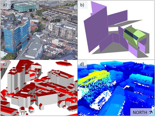
In absence of a 3D city model, if available, one can rely on the DSM data only to take into account the shading effect of the surroundings (see Figure 1). To calculate shading, most building energy and daylight simulation software need a surface geometry representation of the shading obstructions, such as polygons defined with the coordinates of their vertices. An established approach is to generate a 3D surface geometry from the DSM using the Delaunay triangulation algorithm, resulting in a 3D model of the surveyed area (Jakubiec and Reinhart 2013). The 3D geometry can then be imported into a building energy or daylight simulation software to serve as input for representing the surroundings. However, this often requires conversion between different geometry file formats, which is still only partially automated, making it a time-consuming task (Jones, Greenberg, and Pratt 2012). This is especially true, when working with point clouds. Arguably, to date, the most coherent workflow for handling DSM point clouds, building energy and daylight simulation model geometry is offered by Ladybug tools (Roudsari 2017; Roudsari and Pak 2013). However, some modellers or researchers might find the user interface or the paid license for Rhinoceros (Robert McNeel & Associates 2020) a somewhat limiting factor.

Figure 1. Geometry representations of the same area in Eindhoven, the Netherlands from different sources: (a) Aerial view from GoogleMaps (Google 2020), (b) immediate surroundings modelled in SketchUp CAD software (Trimble 2020), (c) GML model (Gemeente Eindhoven 2011), (d) DSM point cloud (Land Registry of the Netherlands, 2020).

In order to expand the toolset of building energy modellers and researchers for taking into account the shading effect of the surroundings, the Point Cloud Based (PCB) 2 phase solar irradiance modelling method is developed and presented in this paper. It is a new method that facilitates the use of DSM point clouds directly as geometry input, combined with a matrix-based approach to model solar irradiance (see Figure 2). Using the DSM data directly as shading input makes the considered shading geometry more up-to-date, since as soon as the DSM is published, the irradiance simulation can already be conducted and there is no reliance on other actors to publish further processed 3D city models.

Figure 2. Schematic workflows for simulating solar irradiance using DSM as shading geometry with the (a) 2 phase (existing state of the art) and the (b) PCB 2 phase (contribution of this paper) methods. A more detailed description of these workflows can be found in Sections 2 and 3.

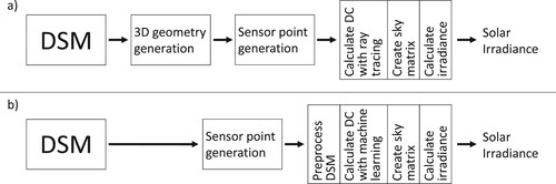
The paper is structured as follows: In Section 2, matrix-based solar irradiance methods are introduced and the theoretical background of the state-of-the-art 2 phase method is described. In Section 3, the main contribution of this paper, the PCB 2 phase method is described alongside an inter-model comparison between the 2 phase and PCB 2 phase methods. Section 4 demonstrates the usability of the PCB 2 phase method in real-world applications, such as, calculating shaded solar irradiance for PV modelling and calculating solar heat gain for building energy modelling using DSM point clouds for shading. In Section 5, conclusions are drawn and the limitations of the proposed method are discussed.

2. Matrix-based solar irradiance simulation methods

Provided that a 3D surface model of the environment is available, ray-tracing is a widely used method to calculate the Plane Of Array (POA) solar irradiance or illuminance both on external and internal surfaces of buildings, taking into account the shading effect and the reflections from the surroundings (Brembilla et al. 2019; Wang, Wei, and Ruan 2020). Radiance is an open-source suite of validated tools to model and render luminous effects of building fenestration and interior lighting (Ward and Shaskespeare 2003). It is less commonly used for such purpose, but Radiance can also model solar irradiance on PV surfaces (Lo, Lim, and Rahman 2015). However, simulation with ray-tracing at every timestep can be time-consuming, especially for (annual) hourly or sub-hourly simulations. In order to reduce computation time for an annual calculation, the concept of the daylight coefficient was introduced in 1983 (Tregenza and Waters 1983). This concept was later developed further, by introducing multiple phases to the calculation of the flux transfer matrix between the sensor point¹ and the discretized sky² (Subramaniam 2017a) in order to speed up calculations, increase the spatial resolution or add the capability of modelling dynamic scenes.

For modelling solar irradiance on external static built surfaces, perhaps the most fitting method is the 2 phase or the 2 phase DDS method (Bourgeois, Reinhart, and Ward 2008). The multi-phase methods improve on simulation speed by reducing the amount of ray-tracing calculations needed for the annual simulation. Other efforts, such as Accelerad (Jones and Reinhart 2017, 2015), focus on speeding up the ray-tracing simulations themselves. However, ray-tracing based methods can only be used if the 3D model geometry of the surroundings is readily available. The PCB 2 phase method proposed in this paper aims to make solar irradiance modelling more time-efficient by bypassing the ray-tracing steps and more importantly, by using the DSM point cloud directly to calculate daylight coefficients, which eliminate the need for 3D geometry generation. Since the PCB 2 phase method builds on the 2 phase method, in the next subsections, the 2 phase method is described first, then the PCB 2 phase method is described in section 3.

2.1. The 2 phase method

2.1.1. Background

The 2 phase method (or daylight coefficient method) is based on the recognition that the irradiance at a given sensor point is determined by the radiance of the sky and the geometry and optical properties of the surroundings and while the sky conditions change at every time step, the surroundings of a sensor point (e.g. a city around a rooftop) are usually static (Brembilla and Mardaljevic 2019). The simulation can therefore be separated into two phases: generating a daylight coefficient vector (i.e. a list of daylight coefficient values) and a sky vector (i.e. a list of radiance values for the segments of a discretized sky). The daylight coefficient vector describes the flux-transfer relation between a luminous sky segment and a sensor point (Tregenza and Waters 1983)³ (1) $\mathrm{\Delta }{I}_{\alpha }=D{C}_{\alpha }\ast L_{\alpha }\ast \mathrm{\Delta }{S}_{\alpha }$(1) where $\mathrm{\Delta }{I}_{\alpha }$ is the irradiance contribution of the αth sky segment [W/m²] $D{C}_{\alpha }$ is the daylight coefficient of the αth sky segment [-] $L_{\alpha }$ is the radiance of the αth sky segment [W*sr^-1*m^-2] $\mathrm{\Delta }{S}_{\alpha }$ is the angular size of the αth sky segment [sr] The calculated $I_{SP}$ irradiance at the sensor point at a given timestep can be obtained by adding up the $\mathrm{\Delta }{I}_{\alpha }$ irradiance contributions from all sky segments. For annual calculations, instead of a sky vector, one can use a sky matrix (a list of lists of sky segment radiance values) to calculate $I_{SP}$. To do this, a discretized sky needs to be created for each timestep (see next sub-section), but the most time-consuming part of the simulation, which is calculating the daylight coefficients with ray-tracing, still just has to be done once.

2.1.2. Modelling the discretized sky

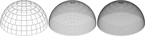
A discretized sky is a numerical approximation of a continuous sky model (Subramaniam and Mistrick 2018). In this work, the Tregenza sky division method (sometimes also called Reinhart sky discretization) (McNeil 2014a) is used, which is the most common discretization for daylight coefficient calculations. The spatial accuracy of the 2 phase method increases as the number of sky segments increase. Usually, increasing the sky discretization is done by sub-dividing the sky segments with an MF factor resulting in $144\ast \text{M}{\text{F}}^2+1$ sky patches (see Figure 3).

Figure 3. Sky discretizations with different resolutions: MF1, MF4 and MF6 with 145, 2305 and 5185 sky segments, respectively.

One can use e.g. the Gendaymtx (LBNL 2020a) Radiance sub-program to generate a sky matrix. It takes weather data as input (e.g. pre-processed from an epw weather file) and produces a matrix of sky segment radiance values using the Perez all-weather model (Perez, Seals, and Michalsky 1993). Gendaymtx also calculates a ground radiance value based on the ground albedo which is stored in the sky vector as the 0th sky segment.

2.1.3. Calculating the daylight coefficients with ray-tracing

Calculating the daylight coefficients (apart from a few simple cases) is only feasible in a numerical way. Most daylight simulation software uses Radiance as a simulation engine for calculating the daylight coefficients with ray-tracing. To date, probably the most popular implementation is DAYSIM, but others are also available which build on DAYSIM, such as DIVA4Rhino, and early versions of Ladybug-Honeybee (Subramaniam 2017b). Newer versions of Ladybug-Honeybee already support Radiance-based 2 and 3 phase methods. Since the implementation of new Radiance functions such as Rfluxmtx (LBNL 2020b), calculating daylight coefficients natively in Radiance became simpler to execute in fivesteps:

• (1). Scene geometry generation and pre-processing. This can be done in a CAD software e.g. Trimble SketchUp (Trimble 2020). Material properties (reflectance and specularity) can be defined in a separate material definition file.

• (2). Sensor point generation. The position, tilt and orientation angle of the sensor points needs to be defined in a pts file. This can be done in simple cases with only a few sensor points in a text editor, or with a pre-processing tool, like Pyrano (Bognár and Loonen 2020) or Ladybug-Honeybee (Roudsari 2017).

• (3). Calculating the Daylight coefficients, or more specifically, the flux transfer coefficients ($E=DC\ast \mathrm{\Delta }S$ with the unit $\left[sr\right]$). The calculation of the flux transfer coefficients with ray-tracing happens by placing the sensor point and the model geometry in a uniformly glowing sphere and calculating the relative contribution of each sky segment to the irradiance at the sensor point by binning the ray-contributions based on incidence angle.

• (4). Weather input pre-processing and generating the sky matrix. In this step, the sky matrix is generated from the weather input, which is usually an epw weather file and the output is 8760 sky vectors (together representing the sky matrix) containing the radiance values of their sky segments calculated with the Perez all-weather model.

• (5). Calculating the irradiance time series. This last step consists of multiplying the sky matrix and the flux-transfer vector.

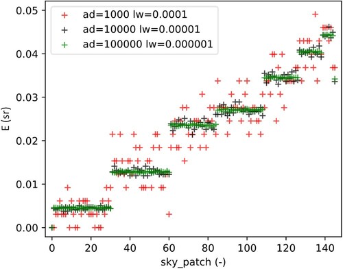
A few key parameters need to be set to find the right balance between accuracy and speed of the flux transfer coefficient calculations with Radiance: m, ab, ad and lw. The m parameter defines the fineness of the Tregenza sky discretization (see Figure 3). ab is the number of considered ray bounces. An ab value of 2 or 3 is sufficient for solar irradiance calculations to be used as input in PV simulations. Higher ab increases simulation time. ad is the number of ambient divisions. Increasing ad increases the number of sampling rays emitted from the sensor point. Higher ad value will lead to less ‘noise’ in the results (see Figure 4). However, if the fineness of the sky discretization is increased in order to reduce noise, ad needs to be further increased as well, which increases simulation time. lw defines a limit to the weight of the ray contributions to avoid tracing rays that would have an insignificant effect on the results. It is recommended to use $lw=1/ad$ (McNeil 2014b).

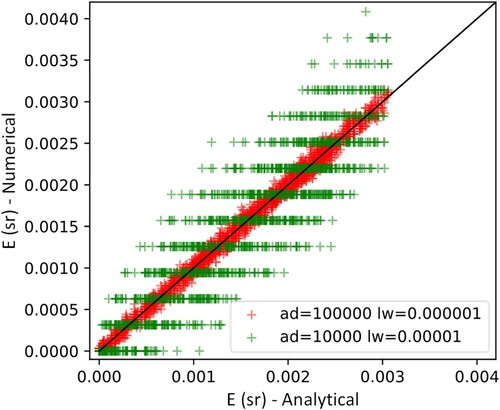
Figure 4. Flux-transfer coefficients calculated with different ad and lw parameters for a sensor point in an empty scene, looking upwards. The exact E values are close to the green data points.

3. The PCB 2 phase method

3.1. Background

The 2 phase method has made calculating solar irradiance in urban environments more efficient, by eliminating the need for conducting ray-tracing for each timestep and converting the effect of the surroundings into a set of coefficients corresponding to each segment of the discretized sky. The 2 phase method utilizes Radiance as a ray-tracer to calculate the flux transfer coefficients. In order to conduct ray-tracing, a surface-based geometry representation and reflectance properties of the environment are necessary as input. However, this input is not always available. It is more and more common that municipalities conduct LiDAR surveys of cities or other urban areas. However, converting the LiDAR point cloud of entire neighbourhoods into a surface model can require a lot of (human) modelling effort and time which limits the usability of these datasets.

The PCB 2 phase method was developed to calculate solar irradiance on external built surfaces using DSM point clouds as shading geometry input. The aim was to adapt the modelling method to the type of input that is available in typical PV or solar heat gain modelling application while preserving sufficient accuracy of the simulation results. In the PCB 2 phase method, the ray-tracing step of the 2 phase method is replaced with three steps: (1) an analytical calculation of the flux-transfer coefficients for an empty scene, (2) a sky segment cover ratio calculation based on the DSM point-cloud projected onto the sky hemisphere and (3) an approximation of diffuse reflected solar irradiance from the surroundings.

3.2. Analytical calculation of the flux-transfer coefficients for an empty scene

To calculate the flux-transfer coefficients for each sky segment, first, the indefinite integral of the irradiance function is determined over a uniformly glowing sphere (with ${\text{L}}_{\varphi \theta }=1\mathrm{W}\ast \mathrm{s}{\text{r}}^{-1}\ast {\text{m}}^{-2}$) sphere around the sensor point using the continuous form of Equation (1) (2) $E_{\mathrm{\Phi }\theta }=\int \int ◯D{C}_{\varphi \theta }\ast L_{\mathrm{\Phi }\theta }\text{d}S$(2) Intuitively, $E$ can be imagined as the volume between the surface of the irradiance function and the unit sphere in Figure 5.

Figure 5. Parametrization of the sky hemisphere.

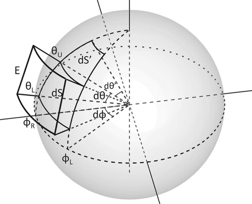
To calculate the integral, one can parametrize the sky hemisphere with the azimuth $\left(\varphi \right)$ and elevation angle $\left(\theta \right)$ thus getting the following equation (3) $E_{\varphi \theta }=\int \int D{C}_{\varphi \theta }\ast L_{\varphi \theta }\ast \text{cos}\theta \text{d}\theta \text{d}\varphi$(3) Note that a new $\text{cos}\theta$ factor got introduced to the equation. This is the consequence of the parametrization: as $\theta$ approaches $\pi /2$, the area of $dS$ approaches 0 which is taken into account with the $cos\theta$ factor. This effect can be observed by comparing $dS$ and $d{S}^{\mathrm{\prime }}$ in Figure 5. The next step is to evaluate Equation (3) with the known parameters, thus we can write (4) $E_{\varphi \theta }=\int \int \text{sin}\theta \ast \text{cos}\theta \text{d}\theta \text{d}\varphi$(4) because ${\text{L}}_{\varphi \theta }=1\mathrm{W}\ast \mathrm{s}{\text{r}}^{-1}\ast {\text{m}}^{-2}$ (the radiance of the uniformly glowing sphere), and because $\text{D}{\text{C}}_{\varphi \theta }=\mathrm{s}\mathrm{i}\mathrm{n}\theta$ in an empty scene for an upwards-looking sensor point, as $\text{D}{\text{C}}_{\varphi \theta }$ is merely determined by Lambert’s cosine law (Tregenza and Waters 1983). One can start solving Equation (4) by starting with the inner integral with respect to $\theta$, then the result can be substituted into Equation (4) to calculate the outer integral with respect to $\varphi$ (5) $\begin{array}{rl}\int -\frac{1}{4}[\cos \left(2\theta \right){]}_{{\theta }_L}^{{\theta }_U}\text{d}\varphi & =-\frac{1}{4}[\cos \left(2\theta \right){]}_{{\theta }_L}^{{\theta }_U}\ast \int 1\text{d}\varphi \\ & =-\frac{1}{4}\left[\cos \left(2\theta \right){]}_{{\theta }_L}^{{\theta }_U}\ast \right[\varphi {]}_{{\varphi }_R}^{{\varphi }_L}\end{array}$(5)

By substituting the bounds according to the Newton–Leibniz axiom one can get (6) $E_{\varphi \theta }=-\frac{1}{4}\ast \left(\cos \left(2{\theta }_U\right)-\cos \left(2{\theta }_L\right)\right)\ast \left({\varphi }_L-{\varphi }_R\right)$(6)

The flux-transfer coefficients of the Tregenza sky segments can be calculated by substituting the left-right azimuths $({\varphi }_L,{\varphi }_R)$ and upper-lower elevations $({\theta }_{\text{U}},{\theta }_L)$ with the azimuths and elevations of the sky segment edges. Figure 6 shows the comparison between the ray-tracing calculated and analytical results. It can be observed that the match is not perfect between the exact analytical solution and the numerical calculation conducted with Radiance. However, the accuracy of the Radiance calculation can be increased (at the expense of longer simulation time) by adjusting ad and lw parameters.

Figure 6. Flux-transfer coefficients calculated for an upward-looking sensor point in an empty scene with a 145 sky segment Tregenza sky division with Radiance (ad=10000, lw=0.00001) and with the analytical calculation (Equation (6)).

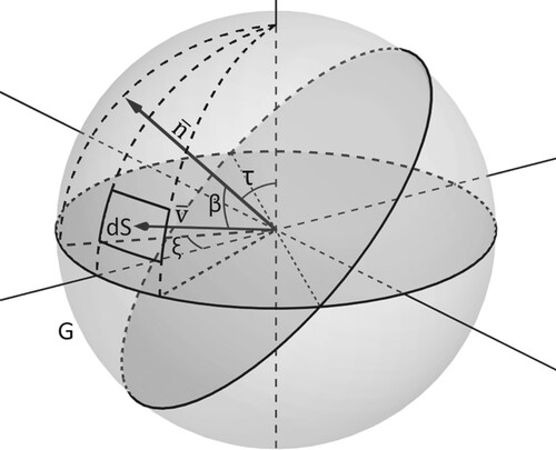
The next step is to generalize the calculation to an arbitrarily tilted sensor point. With the tilted sensor point, the incidence angles change, thus $E$ changes. Also, the ground plane falls into the field of view of the sensor point, therefore, a flux-transfer coefficient for a ground segment needs to be calculated as well. In the case of an arbitrarily tilted sensor point, $\text{D}{\text{C}}_{\varphi \theta }$ is the cosine of the $\text{β}$ angle between the $\overline{n}$ unit vector of the sensor point view angle and the $\overline{v}$ unit vector with $\varphi$ azimuth and $\theta$ elevation (see Figure 7), which can be expressed as (7) $D{C}_{\varphi \theta }=\text{cos}\theta \ast \text{sin}\tau \ast \cos \left(\xi -\varphi \right)+\text{sin}\theta \ast \text{cos}\tau$(7) where $\tau$ is the sensor point unit vector tilt angle [rad] $\xi$ is the sensor point unit vector orientation angle [rad]

Figure 7. Sky hemisphere with the arbitrarily tilted sensor point.

Substituting Equations (7)–(3) and using that ${\text{L}}_{\varphi \theta }=1\mathrm{W}\ast \mathrm{s}{\text{r}}^{-1}\ast {\text{m}}^2$, one gets the following: (8) $\begin{array}{rl}{E}_{\varphi \theta }& =\int \int \left(\text{cos}\theta \ast \text{sin}\tau \ast \cos \left(\xi -\varphi \right)+\text{sin}\theta \ast \text{cos}\tau \right)\\ & \ast \text{cos}\theta \text{d}\theta \text{d}\varphi \end{array}$(8)

After calculating the inner integral of Equation (8) with respect to $\theta$ is and using the trigonometric formulas $co{s}^{2}a=1/2\ast \text{cos}\left(2a\right)+1$ and $\text{cos}a\ast \text{sin}a=1/2\ast \text{sin}\left(2a\right)$ one can write (9) $\begin{array}{rl}& \frac{1}{2}\ast \left(\text{sin}\tau \ast \cos \left(\xi -\varphi \right)\ast \left(\int \cos \left(2\theta \right)\text{d}\theta +\int 1\text{d}\theta \right)\right.\\ & \left.+\text{cos}\tau \ast \int \sin \left(2\theta \right)\text{d}\theta \right)\\ & =\frac{1}{4}\ast [\text{sin}\tau \ast \cos (\xi -\varphi \left)\ast \right(\text{sin}\left(2\theta \right)+2\theta )\\ & -\text{cos}\tau \ast \mathrm{c}\mathrm{o}\mathrm{s}\left(2\theta \right){]}_{{\theta }_L}^{{\theta }_U}\end{array}$(9)

One can substitute the bounds according to the Newton–Leibniz axiom and calculate the outer integral with respect to $\varphi$ (10) $\begin{array}{rl}& \frac{1}{4}\int (\text{sin}\tau \ast \cos (\xi -\varphi )\ast (\text{sin}\left(2{\theta }_U\right)+2{\theta }_U)\\ & -\text{cos}\tau \ast cos\left(2{\theta }_U\right))\\ & -(\text{sin}\tau \ast \cos (\xi -\varphi )\ast (\text{sin}\left(2{\theta }_L\right)+2{\theta }_L)\\ & -\text{cos}\tau \ast cos\left(2{\theta }_L\right))d\varphi \\ & =\frac{1}{4}\ast [\text{sin}\tau \ast \text{sin}(\varphi -\xi )\ast (\left(\text{sin}\left(2{\theta }_U\right)+2{\theta }_U\right)\\ & -\left(\text{sin}\left(2{\theta }_L\right)+2{\theta }_L\right))\\ & -\text{cos}\tau \ast \varphi \ast \left(\text{cos}\right(2{\theta }_U)\\ & -\text{cos}\left(2{\theta }_L\right)){]}_{{\varphi }_R}^{{\varphi }_L}\end{array}$(10)

Substituting the bounds results in the following: (11) $\begin{array}{rl}{E}_{\varphi \theta }& =\frac{1}{4}\ast \left(\text{sin}\tau \ast \mathrm{s}\mathrm{i}\mathrm{n}\right({\varphi }_L-\xi \left)\ast \right(\left(\text{sin}\left(2{\theta }_U\right)+2{\theta }_U\right)\\ & -\left(\text{sin}\left(2{\theta }_L\right)+2{\theta }_L\right))\\ & -\text{cos}\tau \ast {\varphi }_L\ast \left(\text{cos}\left(2{\theta }_U\right)-\text{cos}\left(2{\theta }_L\right)\right))\\ & -\frac{1}{4}\ast \left(\right(\text{sin}\tau \ast \text{sin}\left({\varphi }_R-\xi \right)\ast \left(\right(\text{sin}\left(2{\theta }_U\right)+2{\theta }_U)\\ & -\left(\text{sin}\left(2{\theta }_L\right)+2{\theta }_L\right))\\ & -\text{cos}\tau \ast {\varphi }_R\ast \left(\text{cos}\left(2{\theta }_U\right)-\text{cos}\left(2{\theta }_L\right)\right))\end{array}$(11) Equation (11) gives negative results for the parts of the sky hemisphere that are ‘behind’ the sensor point’s field of view. In those cases, $E_{\varphi \theta }$ should be interpreted as 0. The flux-transfer coefficient for the ground segment (marked with $G$ in Figure 7) can be derived from the view factor (Duffie and Beckman 2013) of the ground segment (12) $E_G=\frac{\pi }{2}\ast \left(1-\text{cos}\tau \right)$(12)

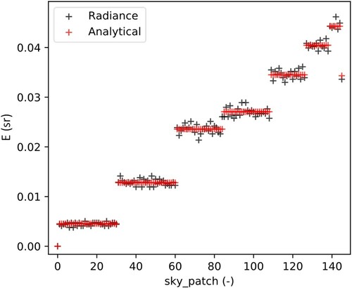
The ray-tracing based, and the analytically calculated flux-transfer coefficients can be compared for a south-facing sensor point with a 45° tilt in Figure 8 with a sky discretization of 2305 sky segments.

Figure 8. Flux-transfer coefficients calculated for a south-facing sensor point with 45° tilt for a 2305-segment sky division with Radiance (numerical) and with the exact (analytical) calculation (Equation (11)). The accuracy of the Radiance calculation can be increased (at the expense of longer simulation time) by adjusting ad and lw parameters.

3.3. Sky segment cover ratio calculation from a DSM point-cloud

With the calculation of the $E$ flux-transfer coefficients for an empty scene (from now on we call this $E_{\text{cos}}$) one can express the flux-transfer relationship between the sensor point and the sky segments determined by Lambert’s cosine law. Next, a method is introduced for taking into account the shading effect of the surrounding geometry with the Cover Ratios (CR) of the sky segments calculated from a DSM point cloud of the surroundings. CR is the angular size of a sky segment that is apparently covered by an obstruction, divided by the angular size of the whole sky segment (13) $\text{CR}=\frac{S_C}{S_S}$(13) where $S_C$ is the covered angular size of the sky segment [sr] $S_S$ is the angular size of the sky segment [sr] The angular size of a sky segment can be calculated similarly to Equation (4) just with 1 instead of $\text{D}{\text{C}}_{\varphi \theta }$ (14) $S_S=\int \int 1\ast \mathrm{c}\mathrm{o}\mathrm{s}\theta \text{ d}\theta \text{d}\varphi =\left[\varphi {]}_{{\varphi }_R}^{{\varphi }_L}\ast \right[\text{sin}\theta {]}_{{\theta }_L}^{{\theta }_U}$(14)

One can get the angular size of the sky segments by substituting the left, right azimuth limits $({\varphi }_L,{\varphi }_R)$ and upper, lower elevation limits $({\theta }_U,{\theta }_L)$ of the sky segments (15) $S_S=\left({\varphi }_L-{\varphi }_R\right)\ast \left(\text{sin}{\theta }_U-\text{sin}{\theta }_L\right)$(15) Calculating $S_C$, on the other hand, is not straightforward without a 3D surface geometry of the surroundings, as the proposed method relies only on the x, y, z coordinates of the surroundings’ DSM point cloud. Calculating the $\text{CR}$ values for a discretized sky is, therefore, a multi-step process:

The first step is pre-processing the DSM point cloud input. This means selecting an appropriate radius around the sensor point where the irradiance is simulated. Only the DSM points within this radius will be included in the simulation. The suitable radius depends on the topology of the urban environment (usually between 200-500 metres), so the selected subset covers all objects (buildings, vegetation) that can potentially shade the sensor point.

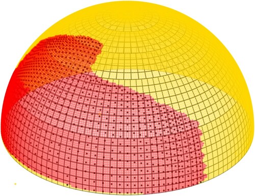
The second step is projecting the point cloud on a unit-sphere around the sensor point. In this step, the DSM point cloud representing the geometry of the surroundings is transformed from the Cartesian coordinate system to a spherical coordinate system where each DSM point is defined by its azimuth, elevation angle, and distance from the centre of the sphere $(\varphi ,\theta ,r\text{)}$. Then, the DSM points can be projected on the unit-sphere, by making $r=1$ or all points. Figure 9 shows the outcome of such projection with artificially generated (1 point per m²) points over a 3D geometry. Projecting the DSM points on the unit sphere can be regarded as a form of parameter reduction since the distance of an object from the sensor point does not influence whether it shades the sensor point, only its apparent position on the sky hemisphere and angular size. Now, that the point cloud on the unit sphere is two-dimensional (i.e. it can be described by merely $\varphi$ and $\theta$ it can be examined together with the discretized sky, in the same coordinate system (see Figure 10).

Figure 9. (left) Geometry of the scene with artificially generated DSM points on it. (right) DSM point cloud of the scene projected to the surface of a unit-sphere around the sensor point.

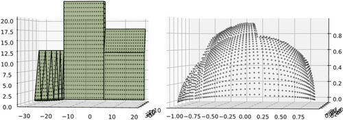
Figure 10. DSM point cloud representation of test-geometry projected to the discretized sky hemisphere with 2305 segments.

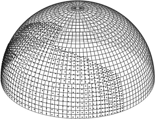
The last step is classifying the sky hemisphere to covered and uncovered areas (by the projected DSM point cloud) and determining the CR of the sky segments. By regarding Figure 10 and using human intuition, one could draw a line around the projected sensor points, indicating the edge of the projected geometry on the sky hemisphere. On one side of the line would be the covered side of the sky hemisphere and the other is uncovered sky. Moreover, one can admit to classifying some sky segments with no projected DSM points in them as covered, because all the other segments around them are covered. Also, one would probably intuitively determine some segments around the edges as partially covered by the DSM point cloud. For an automated calculation of the CR of the sky segments one would need a similar ‘intuitive’ classification of the sky hemisphere to covered and uncovered areas executed by the computer. Since the number and distribution of the projected DSM points are rather unpredictable (determined by the quality of the DSM point cloud) a generalization method is needed, to determine the CR of the sky segments. To do this, Support Vector Machine (SVM) classification is used (see the appendix) to divide the sky hemisphere into covered and uncovered areas. Since SVM is a supervised machine learning method, a labelled training dataset is needed. The projected DSM point cloud (with $\varphi ,\theta$ features) labelled as covered sky points is used as training data representing the covered sky area. For uncovered training data, one can generate a uniform grid of sky points (see Figure 11).

Figure 11. The training dataset of the SVM model. Black points are the training points labelled as covered (this is the projected DSM point cloud) and the blue points are the sky points (a uniform grid of points generated to represent the sky).

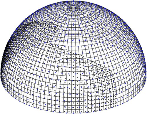
Together, these points on the sky hemisphere represent the training data for the SVM model. Once the model is trained, one can test the sky at any arbitrary position, to determine whether it is in the covered or uncovered area of the sky (see Figure 12). This way, the DSM points on the sky hemisphere can be ‘multiplied’, and the covered fraction of the sky segments becomes quantifiable.

Figure 12. Tested points with the trained SVM model. Red points are classified as covered and the yellow points are classified as uncovered. Black points are the projected DSM points.

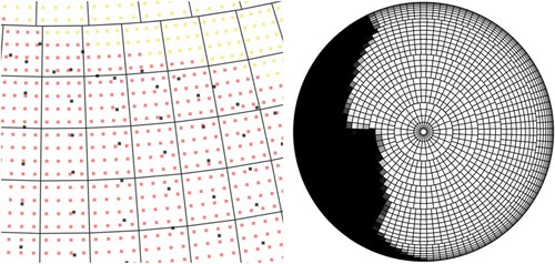
One can choose the locations for testing the sky with the trained SVM in such a way that the quantification of CR is convenient. Figure 13 shows a magnified section of the discretized sky with the projected DSM points and the tested points with the SVM model. There are 4 × 4 tested points in each sky segment, therefore CR or a given sky segment can be calculated as (18) $\text{CR}=\frac{n_C}{n_S}$(18) where $n_C$ is the number of test points classified as covered in the segment [-] $n_S$ is the number of test points in the segment [-]

Figure 13. (left) Magnified section of Figure 12: Tested points with the trained SVM model. Red points are classified as covered and the yellow points are classified as uncovered. Black points are the projected DSM points. (right) CR values visualized on the sky hemisphere. Black indicates a CR of 1, white indicates 0.

3.4. Approximating reflected solar irradiance

With $E_{\text{cos}}$ and CF, one can take into account the cosine effect and the shading from the surroundings. A last component that needs to be added to the model is the contribution of the reflected component $E_r$ to the flux-transfer coefficients. As the geometry input is merely a DSM point cloud without surfaces, the surface normals are not available, and therefore, it cannot be determined at which angle a light ray would bounce off the geometry. The PCB 2 phase method is therefore not suitable for calculating the reflected irradiance from specular surfaces, as in those cases the surface normals are a necessary input. Instead, it is assumed that the surrounding geometry is diffusely reflective (which is a commonly used assumption in practice), and two methods are proposed to approximate the re-distribution of $E_r$ over the sky hemisphere using a uniform ϵ albedo for the surroundings.

Figure 14(a,b) show simplified diagrams of determining the change in the flux-transfer coefficient of the sky segments with specular and diffuse reflections using the 2 phase method. This is done by finding the source sky segment of the reflected light with ray-tracing. In the specular case, the sampling ray is reflected from the surface according to the law of reflection before it hits a sky segment. As a result, the $E$ of the sky segment increases. In the diffusely reflective case, when a sampling ray hits a diffuse surface, new sampling rays are generated in all directions in front of the plane of the surface. Where these new sampling rays hit the sky segments, the $E$ increases. This can also be observed with the 2 phase method simulation results in Figure 15(a,b) which show the change in $E$ due to reflections compared to $E_{\text{cos}}$. Blue indicates a decrease and red an increase in $E$, while white indicates no change (no reflected sampling rays hit those sky segments).

Figure 14. Schematic diagram of the workings of identifying the source of the reflected light with (a) Ray-tracing for specular surfaces, (b) Ray-tracing for diffusely reflective surfaces, (c) PCB 2 phase method with the Uniform re-distribution reflection approximation and (d) PCB 2 phase method with the Opposite side re-distribution reflection approximation. Blue arrows on the sky hemisphere represent ${\text{E}}_{\text{cos}}$ yellow ones represent ${\text{E}}_{\text{r}}$.

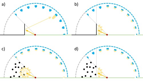
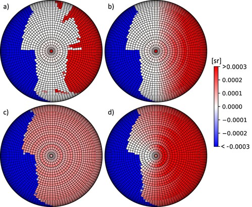
Figure 15. Diagrams showing the change in E for each sky segment of a 2305-discretized sky due to reflected light compared to ${\text{E}}_{\text{cos}}$ for an upwards-looking sensor point. Blue indicates decrease, red increase in $\text{E}$while white indicates no change. (a) and (b) cases were simulated with the 2 phase method (with ray-tracing) using the 3D geometry shown in Figure 17 with a specular and diffuse albedo of 0.5. (c) and (d) shows the same output generated with the PCB 2 phase method with the Uniform and the Opposite side re-distribution reflection approximation, where the geometry input was the artificially generated DSM point cloud (as seen in Figure 9).

In the case of the PCB 2 phase method, the direction of the reflections has to be assumed from the point-cloud representation of the surrounding geometry. Two methods are proposed for this purpose

• Uniform re-distribution method. In this case, it is assumed that the obstructions with a given ϵ albedo reflect the light in all directions (at a 4π steradian angle) equally. For each sky segment, first, it is calculated what is the part of $E$ that gets reflected $E_{\text{cos}}\ast CF\ast ϵ$ and then this gets redistributed to all the other sky segments in an area-weighted way. A schematic representation of the workings of this method is shown in Figure 14(c) and simulation results in Figure 15(c).

• Opposite side re-distribution method. In this case, it is assumed that each sky segment only reflects the opposite half of the sky hemisphere (at a 2π steradian angle). For each sky segment with an azimuth angle of $\varphi$, after calculating what is the part of $E$ that gets reflected from it $E_{\text{cos}}\ast CF\ast ϵ$, it is identified, which sky segments are between the $\varphi +{90}^{\circ }$ and $\varphi -{90}^{\circ }$ azimuth bounds, and the reflected $E$ gets distributed among those, in an area-weighted way. A schematic representation of the workings of this method is shown in Figure 14(d) and simulation results in Figure 15(d).

With the methods described above, reflected light can be taken into account when using raw DSM point clouds as geometry input for simulating solar irradiance with the PCB 2 phase method. The two proposed (Uniform and Opposite side) methods for re-distributing the reflected $E$ differ in their assumptions about the surroundings and simulation speed.

3.5. Combining the phases

The irradiance at sensor point ($I_{SP}$) can be calculated by adding up the irradiance contributions of the sky segments (19) $I_{SP}=\sum _{\alpha =0}^n\left(E_{\text{cos},\alpha }\ast \left(1-C{R}_{\alpha }\right)+E_{r,\alpha }\right)\ast L_{\alpha }$(19) where $I_{SP}$ is the irradiance at the sensor point [W/m²] $n$ is the number of sky segments (the 0^th segment is the ground) [-] $E_{\text{cos},\alpha }$ is the flux-transfer coefficient of α sky segment for an empty scene [sr] $C{R}_{\alpha }$ is the cover ratio of α sky segment [-] $E_{r,\alpha }$ is the reflected component of the flux-transfer coefficient for α sky segment [sr] $L_{\alpha }$ is the radiance of the α sky segment [W*sr^-1*m^-2]

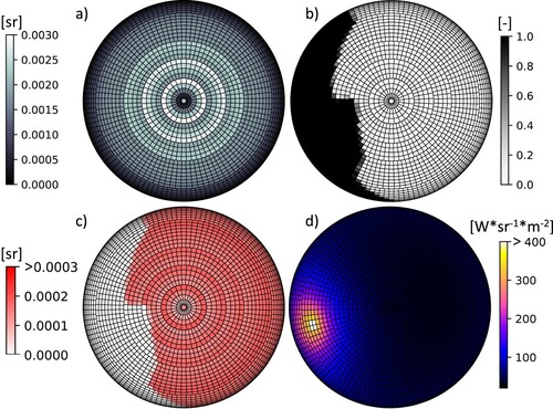
Figure 16 shows the ${\text{E}}_{\text{cos},\alpha }$, $\text{C}{R}_{\alpha }$, ${\text{E}}_{\text{r},\alpha }$ and ${\text{L}}_{\alpha }$ values plotted on the discretized sky hemisphere for the geometry shown in Figure 9.

Figure 16. Values of (a) ${\text{E}}_{\text{cos}}$, (b) $\text{CR}$, (c) ${\text{E}}_{\text{r}}$ plotted on the discretized sky hemisphere for an upward-looking sensor point with the geometry shown in Figure 9, and (d) $\text{L}$ sky segment radiance values (at 16:00 on the 26th of May in Amsterdam based on an IWEC weather file).

3.6. Inter-model comparison of 2 phase and PCB 2 phase solar irradiance modelling methods

To compare the simulated solar irradiance with the 2 phase and the PCB 2 phase methods, the model geometry (shown in Figure 17), and an artificially generated point cloud (shown in Figure 9) are used. The model geometry consists of diffusely reflective surfaces and a ground plane. The simulations are conducted at one position, with four different azimuths and tilts 90-90, 180-0, 180-45 and 270-0 degrees, respectively. This is to ensure that the two methods are compared under various circumstances, as the tested sensor points have different amounts of obstruction, ground and sky in their field of view.

Figure 17. Geometry of the scene with the four sensor points, all located at the origin of the coordinate system. The orientation and tilt angles of the sensor points are 90-90, 180-0, 180-45, 270-0 degrees for the cyan, red, green and yellow sensor points respectively.

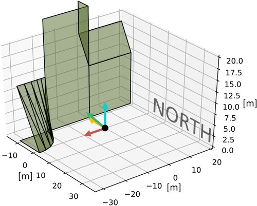
Figure 18 shows solar irradiance simulation results with the two methods on a sunny day, without taking into account reflected light using a black model geometry $ϵ=0$. This comparison assesses the geometric fidelity of the PCB 2 phase method to represent the geometry of the surroundings with the Cover Ratios, based on a DSM point cloud. It can be concluded, that the direct and diffuse shading calculated with the PCB 2 phase method matches very closely to the result of the 2 phase method.

Figure 18. Simulated solar irradiance with the 2 phase (solid line) and the PCB 2 phase (dashed line) method for the four sensor points, with black ground and surroundings, on the 31st of March in Amsterdam based on an IWEC weather file.

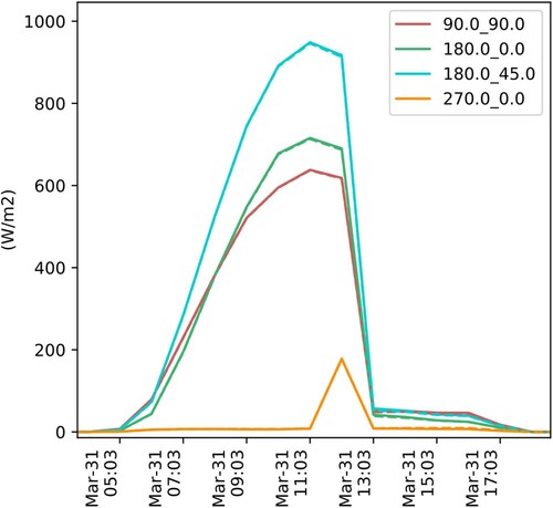
Figure 19 shows a comparison of simulated solar irradiance with grey diffusely reflective $ϵ=0.5$ round plane and surroundings. Here, three methods are compared: the 2 phase method, the PCB 2 phase method considering the reflected light with the uniform re-distribution method (UD), and lastly the PCB 2 phase method with the opposite side re-distribution method (OSD) (see Section 3.4). By comparing the results in Figure 18 with the ones in Figure 19 it can be seen that the simulated irradiance is higher in the latter case as there the reflected irradiance is also contributing to the results. Most notably, significant differences between the black and the grey models can be observed for the sensor point facing west $\text{(azimuth}={270}^{\circ },\text{elevation}=0^{\circ })$. This sensor point is looking directly at the obstruction and its field of view is almost entirely filled with buildings and the ground plane. Therefore, most of its irradiance is coming from the reflected component. It can be seen that in the morning the 2 phase result matches very closely with the PCB 2 phase OSD results. This is because the assumption used for the OSD method (reflecting the light diffusely from the opposite of the sky hemisphere) matches very closely with reality when the sun is en face with the vertical façade in the simulation model. On the other hand, when the sun moves to the south around noon, the difference between the 2 phase and the PCB 2 phase OSD results increases somewhat. The PCB 2 phase UD method underpredicts the irradiance in the morning, by 10-20% and provides a better match when the sun is in sight or behind the obstruction in the afternoon. In the other – for PV applications more realistic – cases, the match between the 2 and PCB 2 phase results is good for both the UD and OSD versions (maximum deviation is 13% on a timestep level and less than 2.5% on a daily level). A good match can also be observed on a cloudy day in Figures 20 and 21, which shows the yearly simulated solar irradiance with the different discussed methods.

Figure 19. Simulated solar irradiance with the 2 phase (solid line) and the PCB 2 phase-UD (dashed line) and 2 Phase-OSD (dotted line) methods for the four sensor points, with grey ground and surroundings $(ϵ=0.5)$ on the 31st of March in Amsterdam based on an IWEC weather file.

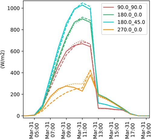
Figure 20. Simulated solar irradiance with the 2 phase (solid line) and the PCB 2 phase-UD (dashed line) and 2 phase-OSD (dotted line) methods for the four sensor points, with grey ground and surroundings $(ϵ=0.5)$ on a cloudy day of April 5th in Amsterdam based on an IWEC weather file.

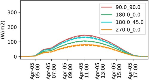
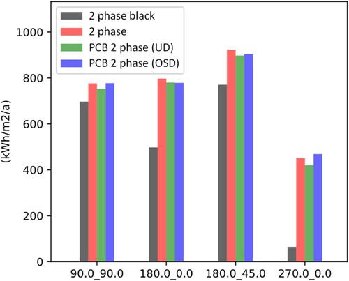
Figure 21. Yearly simulated solar irradiation with the 2 phase (red), the PCB 2 phase-UD (green) and the PCB 2 phase-OSD (blue) methods for the four sensor points, with grey ground and surroundings $(ϵ=0.5)$ based on an IWEC Amsterdam weather file. The 2 phase simulation without reflected component (black) simulation output is also provided for reference.

3.7. Discussion

Based on the above-described case study, it can be concluded that the PCB 2 phase method can simulate the solar irradiance within a few percent accuracy compared to the 2 phase method. An advantage of the PCB 2 phase method over the 2 phase is simpler model input: the DSM point cloud can directly be used as shading obstruction input without the need for generating a 3D surface geometry. A drawback of the method is the incapability of simulating specular reflections, as simulating those would require knowledge about surface normals which are not available without a 3D surface model. However, one could argue that triangulation methods (such as Delauney, ball-pivoting and Poisson) are also often not able to accurately determine the surface normals.

4. Demonstration of the applicability of the PCB 2 phase method

This section demonstrates the real-world application of the PCB 2 phase method with two case studies. In the first case, the PCB 2 phase method is used to calculate the impact of shading on a PV system. In the second case, the effect of surrounding buildings on the solar heat gain, and thus on the heating and cooling demand of a building is investigated. In both cases, openly available DSM point clouds are used as shading geometry input. While the inter-model comparison in Section 3.6 intended to compare the accuracy of the proposed method to the state of the art 2 phase method with the same shading geometry, the case studies in this section are developed to show the importance of incorporating the shading effect of the surroundings when simulating PV or solar heat gains as opposed to ignoring shading.

4.1. Effect of shading on PV performance modelled with the PCB 2 phase method

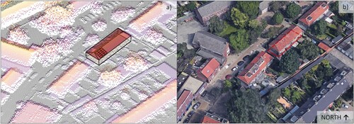
To demonstrate the real-world usability of the PCB 2 phase method for simulating the effect of shading on PV systems, a case study is used in Eindhoven, the Netherlands. Figure 22 shows the 3D model geometry of the building, matched with the corresponding DSM point cloud. The DSM point cloud used for this case study is openly available from the PDOK portal (Land Registry of the Netherlands 2020).

Figure 22. (a) 3D model geometry of a building placed in the corresponding DSM point cloud. (b) Aerial view of the same building and surroundings.

The case study building has a PV system installed on its South-East oriented roof consisting of 12 series-connected PV modules with 10 × 6 PV cells, 3 bypass diodes and 310 W nominal power each. The shaded solar irradiance is calculated for each PV cell with the PCB 2 phase method (see Figure 23 for the sensor-point layout) following the steps described in Section 3. The Pyrano Python package (Bognár and Loonen 2020) was used to pre-process the point cloud, the model geometry and to execute the simulations. The simulated solar irradiance on the PV cells was used as input to simulate the PV yield with PVMismatch (Mikofski, Meyers, and Chaudhari 2018), which is an explicit IV & PV curve calculator for PV system circuits.

Figure 23. (a) 3D model geometry of the case study building with the PV system on it. (b) The PV system with the irradiance sensor points generated for each PV cell.

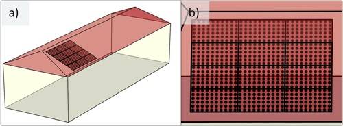
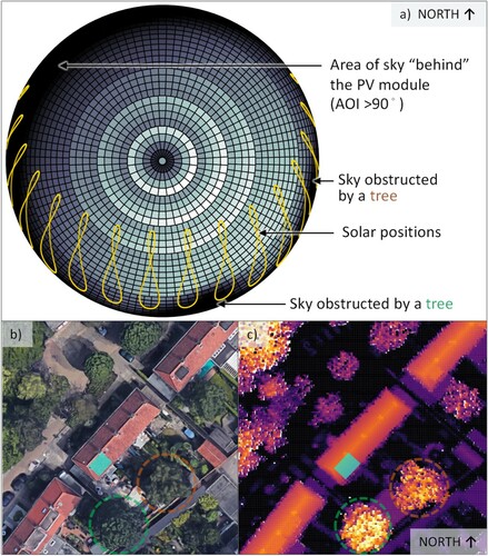
Figure 24(a) shows the calculated mean flux-transfer coefficients for the sensor points generated over the PV system. Note that the features of the surroundings (marked in Figure 24(b,c)) can be recognized on the calculated flux-transfer coefficient values plotted to their corresponding sky segment. It can be also observed that the segments of the sky that is outside of the 180˚ field of view of the PV modules do not contribute to the POA irradiance of the sensor points.

Figure 24. (a) Flux transfer coefficient values visualized on the sky hemisphere. The darker-lighter colours showing lower-higher values respectively. (b) Aerial view of the surroundings. The location of the PV system is indicated with a turquoise rectangle. (c) Height map of the DSM of the surroundings.

The effect of the shading can be observed in Figure 25, where the shaded and unshaded mean POA solar irradiance on the PV cells is compared. The graph shows a clear and overcast day in February. Evidently, the effect of shading on overcast days is negligible, due to the absence of direct solar irradiance. On the other hand, shading from the surrounding trees cause a significant reduction in solar irradiance on clear days. To provide an annual overview, Figure 26 shows the simulated hourly mean solar irradiance on the PV cells and the simulated PV yield resampled to monthly aggregated values. The effect of shading is higher in the transition and winter months than in the summer months. This is due to the lower solar elevation angles in the winter as opposed to the summer months, when due to high solar elevations, the obstructions do not ‘get in the way’ of direct solar irradiance. This is in accordance with what was observed based on the flux-transfer coefficients of the sky segments in Figure 24.

Figure 25. Simulated shaded (s_irr) and unshaded (ns_irr) mean POA solar irradiance on the PV cells on a clear and overcast day in February.

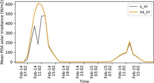
Figure 26. (a) Simulated monthly shaded (s_irr) and unshaded (ns_irr) solar irradiance on the PV cells. (b) Simulated monthly shaded (s_dc_power) and unshaded (ns_dc_power) DC power of the PV system.

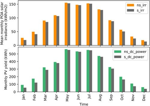
It can also be observed that the difference between the shaded and unshaded simulated DC PV yield is larger than the difference between the shaded and unshaded solar irradiance. This is due to the additional performance loss of the PV systems caused by partial shading (Bognár, Loonen, and Hensen 2019). On a yearly level, the simulated unshaded and shaded PV yield is 3801 and 3520 kWh respectively, thus ignoring the shading effect from the surroundings would cause an 8% overprediction in the simulated annual PV yield in this case. With an increasing interest for battery charging and better matching between energy demand and onsite generation, the timing of PV electricity generation becomes more important than only the annual yield. In such cases, it is expected that the added value of accounting for partial shading will only be more pronounced.

4.2. Effect of shading on building solar heat gains modelled with the PCB 2 phase method

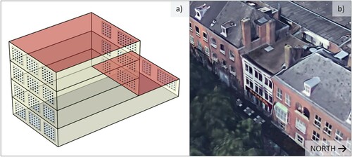
In the case study shown in this section, the effect of shading by the surroundings on the heating and cooling loads of a building is demonstrated. The case study building is located in the city centre of Eindhoven, the Netherlands (see Figure 27). The building has windows in the South-East and North-West facades and is shaded by trees and neighbouring buildings. Some of the most important parameters of the building model are summarized in Table 1. The weather input is an IWEC Amsterdam hourly weather file.

Figure 27. (a) Height map of the DSM and (b) aerial view of the case study building and its surroundings. Green rectangle indicates the location of the building in question.

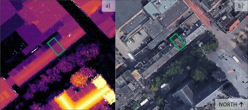
Table 1. Case study model parameters.

External walls U-value (W/m^2K)	0.177	Total floor area (m^2)	312.5
Flat roof U-value (W/m^2K)	0.143	Heating setpoint/setback (˚C)	21/12
Ground floor U-value (W/m^2K)	0.218	Cooling setpoint/setback (˚C)	24/28
External glazing U-value (W/m^2K)	2.665	Air change rate (ACH)	0.2
External glazing SHGC (-)	0.703	Internal heat gains (W/m^2)	2.5

The building energy simulations are conducted with EnergyPlus (Crawley et al. 2000), which by default uses its built-in shading module to calculate the sunlit fraction of the building surfaces from a 3D model of shading geometry, which is in turn used to calculate the solar heat gains through building fenestration. Recent efforts (Hong and Luo 2018) made it possible to outsource the sunlit fraction calculation from EnergyPlus to external software. This means that the sunlit fraction calculations of an EnergyPlus model can be executed with the PCB 2 phase method and imported into EnergyPlus which makes it a convenient method to calculate the solar heat gain of buildings using DSM point clouds as geometry input. Until this point, it was demonstrated how the PCB 2 phase method can be used to calculate solar irradiance at distinct sensor points. To calculate the sunlit fraction of the external glazing surfaces, first the EnergyPlus model geometry is imported into Pyrano and a sensor point grid is generated over the glazing surfaces in a similar way as it was done for the PV modules in section 4.1. Figure 28 shows the sensor point grids over the windows of the EnergyPlus model.

Figure 28. (a) 3D model of the case study building with the irradiance sensor points indicated on the windows. (b) External view of the façade.

The sunlit fraction of a surface can be calculated from the cover ratio (see Section 3.3) in the following way: firstly, the mean cover ratio for each sky segment $C{R}_{m,\alpha }$ is calculated over the sensor points corresponding to the given surface. Then, at every time step (t), it is determined in which sky segment (s) the sun is located. The sunlit fraction of the surface at the given time step is: $1-C{R}_{m,s,t}$. 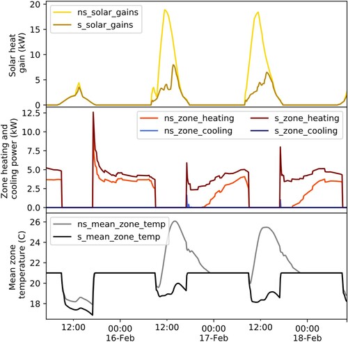Once the sunlit fraction is determined for each window in the model, the sunlit fraction values are imported into EnergyPlus using a ‘Schedule:File:Shading’ EnergyPlus object to run annual simulations. Figure 29 shows the total solar heat gain, the heating and cooling load and the mean air temperature of the case study building, with and without the effect of shading by the surroundings on three consecutive days in February. On an overcast day (15^th of February), the heating loads of the shaded and not shaded cases are similar due to the similar (lack of) solar heat gains. On a sunny day, however, higher heating demand can be observed for the case with shading.

Figure 29. Simulated solar heat gain, heating/cooling load and mean air temperature of the case study building. The graphs show a comparison between the models with and without the shading effect of the surroundings. ‘s' prefix indicates the results with shading and ‘ns' indicates the results without shading.

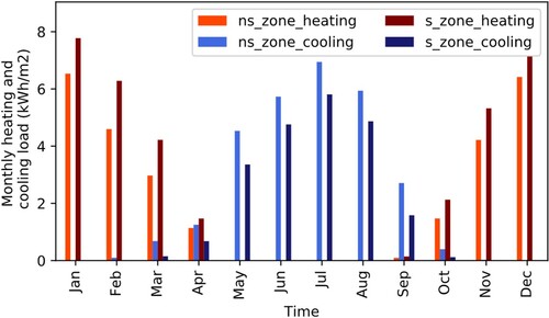
Similar trends can be observed on a monthly level. Figure 30 shows the monthly cumulative heating and cooling loads of the case study building. Shading from the surroundings increases the heating demand and reduces the cooling demand of the building. On a yearly level, the heating demand is 27 and 34 kWh/m² and the cooling demand is 28 and 21 kWh/m² for the unshaded and shaded cases respectively. Therefore, ignoring shading from the surroundings would cause a 21% underprediction of the annual heating demand and 33% overprediction of the annual cooling demand in this case.

Figure 30. Monthly cumulative heating and cooling load normalized with the floor area of the case study building. ‘s' prefix indicates the results with shading and ‘ns' indicates the results without shading.

5. Conclusions

In order to aid the process of taking into account the shading effect of the surroundings, the PCB 2 phase solar irradiance modelling method was developed. The PCB 2 phase method uses DSM point clouds as shading geometry, combined with a matrix-based approach to model solar irradiance. The open-source implementation of the method is available in the Pyrano Python package (Bognár and Loonen 2020). The PCB 2 phase method was compared to a state-of-the-art approach in Section 3.6, where it was found that it can simulate solar irradiance within a few percent accuracy compared to the 2 phase method when simulated with the same shading geometry.

The presented method can simplify the modelling process as the 3D model generation step can be bypassed with it. Moreover, 3D city models often do not include trees and other non-building shading obstructions, which are in turn captured with the PCB 2 phase method. The method can be applied for taking into account the shading effect of the surroundings when calculating interior daylight conditions, PV yield and solar heat gains of buildings. In Section 4, the latter two cases were demonstrated with real-world case studies conducted for determining the effect of shading on PV performance and heating-cooling loads of a building.

5.1. Limitations

The following limitations should be considered when using the PCB 2 phase method:

• The method can only be applied at places where an up-to-date DSM point cloud of the surroundings is available, with sufficient resolution $(\le 0.5\text{m})$.

• The PCB 2 phase method can estimate the amount of the reflected light from the surrounding surfaces, but it cannot calculate its orientation, thus it uses the assumption that the shading obstructions diffusely reflect the light in all directions (at a 4π steradian angle) or to just one half of the sky hemisphere (at a 2π steradian angle) depending on which reflection approximation method is used, as described in section 3.4. On one hand, as many obstructions (walls, roofs of buildings, vegetation) are diffusely reflective, this assumption results in a good approximation of reflected light from most built surfaces. On the other hand, since the PCB 2 phase method does not have means to calculate specular reflections, in case of surroundings with mostly specular-reflective surfaces (e.g. fully glazed buildings, or polished metal facades) the reflected component of the simulated POA irradiance cannot be reliably simulated.

• One cannot assign different reflectance properties to different shading obstructions as only one reflectance can be set for the entire point cloud and one for the ground plane.

• When calculating the shaded POA solar irradiance with the PCB 2 phase method, there are a number of parameters that are needed to be set. These parameters control the sky discretization and the criteria for the SVM classifications. In this paper, for a DSM with 0.5 m resolution the $C=1$, and $\gamma =50$ parameters (see the appendix) and 1296 evenly distributed sky points (see section 3.3) were used for the SVM classification. It is possible that when working with different inputs than the ones used in this paper (e.g. DSM with a different resolution) these parameters are needed to be retuned.

Acknowledgements

We would like to acknowledge Kristóf Horváth from the Budapest University of Technology for enlightening discussions about sphere parametrization.

Disclosure statement

No potential conflict of interest was reported by the author(s).

Additional information

Funding

This work has been supported by the project ‘PV OpMaat’, financed by the cross-border collaboration programme Interreg V Flanders-Netherlands with the financial support of the European Regional Development Fund (CCI 2014TC16RFCB046).

Notes

1 A sensor point is defined by its location [x, y, z] and its orientation vector [xi, yi, zi]. The field of view of a sensor point is 2π steradians.

2 Discretized skies are explained in Section 2.1.2.

3 Note: In Tregenza and Waters’ article they defined Equation (1) with photometric units: illuminance [cd*sr/m²] for $\mathrm{\Delta }{I}_{\alpha }$ and luminance [cd/m²] for $L_{\alpha }$. In this paper, radiometric units are used: irradiance [W/m²] for $\mathrm{\Delta }{I}_{\alpha }$ and radiance [W*sr^-1*m^-2] for $L_{\alpha }$.

Appendix

Machine learning can be defined as the process of solving a practical problem by firstly gathering a dataset, then algorithmically building a statistical model based on that dataset. The built statistical model then is used to solve the practical problem in question. Machine learning techniques can be divided into four categories: supervised, semi-supervised, unsupervised and reinforcement learning (Burkov 2019). In this work, we use Support Vector Machines (SVM) to solve classification problems in Section 3.3. SVMs are in the group of supervised learning techniques. Supervised learning methods take labelled data points with known features as training data to produce a model. Then when we give the model features as input, it will return the corresponding labels as output.

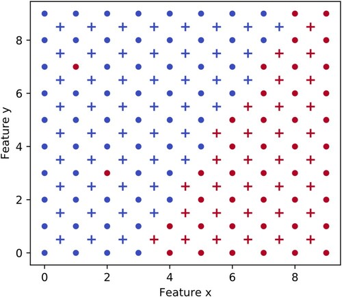
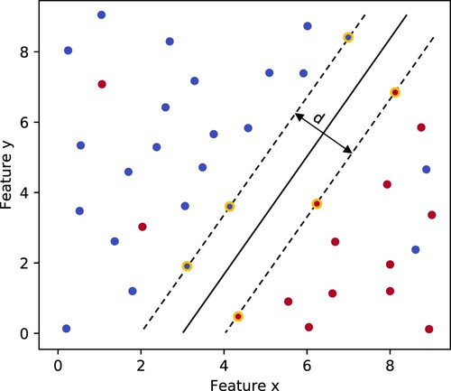
Figure A1 shows a schematic example of classification with SVMs. Each training point is characterized by two features (Feature x and Feature y) and a label (+) or (−). These points are used to train the SVM, and as a result, a hyperplane is identified that divides the points into two classes, following the widest street approach, that is, the dividing line is as far from the divided clusters as possible.

Figure A1. Example of a 2D-separable classification problem. The support vectors are marked with yellow, which define the largest separation (d) between the red and blue classes Adapted from Cortes and Vapnik (1995).

In cases, when the training data is not linearly separable, the decision surface has to be nonlinear. This can be achieved by transforming the training data to a different n-dimensional feature space with a kernel function, where the points are linearly separable with an n-1 dimension hyperplane. In this paper the Radial Basis Function (RBF) was used, implemented in Python, using the Scikit-learn package (Pedregosa et al. 2012). The RBF kernel allows for a non-linear soft-margin classification, where $C$ is a parameter for the soft-margin cost function that allows for adjusting the trade-off between misclassifying a training point and having an overfitted decision surface. $\gamma$ determines the radius of a training point, in which it has an influence on the SVM model. A small $\gamma$ allows for more isolated ‘islands’ of classes in the feature space.

After training the SVM, new data points can be classified into the (+) or (-) classes based on their features. This is indicated in Figure A2. In the concrete case of the PCB 2 phase method, Feature x is the solar azimuth, Feature y is the solar elevation. The labels of the data points are either ‘shaded’ or ‘not shaded’. Due to the soft-margin nature of the used SVM classification method, the prediction is not sensitive to individual, erroneously introduced training points. It is expected, that faulty training points occur in a randomly scattered way in the feature space, therefore with correctly tuned $C$ and $\gamma$ parameters, they do not influence the prediction.

Figure A2. Training (•) and predicted (+) data points on the x–y feature space.

References

- Al-Sallal, K. A., and L. Al-Rais. 2012. “A Novel Method to Model Trees for Building Daylighting Simulation Using Hemispherical Photography.” Journal of Building Performance Simulation 6: 38–52. doi:https://doi.org/10.1080/19401493.2012.680496
- ArcGIS. 2019. “ArcGIS Eindhoven 3D City Model [WWW Document].” https://www.arcgis.com/home/item.html?id=856f7735749b4c41abd1d01eb2b76092.
- Bianchi, C., M. Overby, P. Willemsen, A. D. Smith, R. Stoll, and E. R. Pardyjak. 2020. “Quantifying Effects of the Built Environment on Solar Irradiance Availability at Building Rooftops.” Journal of Building Performance Simulation 13: 195–208. doi:https://doi.org/10.1080/19401493.2019.1679259
- Biljecki, F., H. Ledoux, and J. Stoter. 2017. “Computers, Environment and Urban Systems Generating 3D City Models Without Elevation Data.” Computers, Environment and Urban Systems 64: 1–18. doi:https://doi.org/10.1016/j.compenvurbsys.2017.01.001
- Bognár, Á, and R. C. G. M. Loonen. 2020. “Pyrano [WWW Document].” https://gitlab.tue.nl/bp-tue/pyrano.
- Bognár, Á, R. C. G. M. Loonen, and J. L. M. Hensen. 2019. “Modeling of Partially Shaded BIPV Systems – Model Complexity Selection for Early Stage Design Support.” In Proceedings of the 16th IBPSA Conference, 4451–4458. Rome, Italy: IBPSA.
- Bourgeois, D., C. F. Reinhart, and G. Ward. 2008. “Standard Daylight Coefficient Model for Dynamic Daylighting Simulations.” Building Research & Information 36: 68–82. doi:https://doi.org/10.1080/09613210701446325
- Brembilla, E., D. A. Chi, C. J. Hopfe, and J. Mardaljevic. 2019. “Evaluation of Climate-Based Daylighting Techniques for Complex Fenestration and Shading Systems.” Energy and Buildings 203. doi:https://doi.org/10.1016/j.enbuild.2019.109454
- Brembilla, E., and J. Mardaljevic. 2019. “Climate-Based Daylight Modelling for Compliance Verification: Benchmarking Multiple State-of-the-Art Methods.” Building and Environment 158: 151–164. doi:https://doi.org/10.1016/j.buildenv.2019.04.051
- Brito, M. C., S. Freitas, S. Guimarães, C. Catita, and P. Redweik. 2017. “The Importance of Facades for the Solar PV Potential of a Mediterranean City Using LiDAR Data.” Renewable Energy 111: 85–94. doi:https://doi.org/10.1016/j.renene.2017.03.085
- Brito, M. C., N. Gomes, T. Santos, and J. A. Tenedo. 2012. “Photovoltaic Potential in a Lisbon Suburb Using LiDAR Data.” Solar Energy 86: 283–288. doi:https://doi.org/10.1016/j.solener.2011.09.031.
- Burkov, A. 2019. The Hundred-Page Machine Learning Book. Andriy Burkov.
- CGTrader. 2020. “CGTrader Eindhoven 3D City Model [WWW Document]. https://www.cgtrader.com/3d-models/exterior/cityscape/eindhoven-city-and-surroundings.
- Cortes, C., and V. Vapnik. 1995. “Support Vector Networks.” Machine Learning 20: 273–297. doi:https://doi.org/10.1007/BF00994018
- Crawley, D. B., L. K. Lawrie, C. O. Pedersen, and F. C. Winkelmann. 2000. “EnergyPlus: Energy Simulation Program.” ASHRAE Journal 42: 49–56.
- Department for Environment Food & Rural Affairs. 2020. “Defra Data Services Platform [WWW Document].” https://environment.data.gov.uk/DefraDataDownload/?Mode=survey.
- Duffie, J. A., and W. A. Beckman. 2013. Solar Engineering of Thermal Processes. Hoboken, NJ: John Wiley & Sons.
- Gemeente Eindhoven. 2011. “3D GML Stadsmodel Eindhoven [WWW Document].” https://data.eindhoven.nl/explore/dataset/3d-stadsmodel-eindhoven-2011-gml/information/.
- Google. 2020. “Case Study Location [WWW Document].” https://www.google.nl/maps/place/Eindhoven/@51.4406904,5.4820198,86a,35y,279.61h,55.77t/data=!3m1!1e3!4m5!3m4!1s0(47c6d91b5579c39f:0xf39ad2648164b998!8m2!3d51.441642!4d5.4697225.
- Hong, T., and X. Luo. 2018. “Modeling Building Energy Performance in Urban Context.” In: 2018 Building Performance Analysis Conference and SimBuild Co-Organized by ASHRAE and IBPSA-USA, 100–106. Chicago, IL.
- Jakubiec, J. A., and C. F. Reinhart. 2012. “Towards Validated Urban Photovoltaic Potential and Solar Radiation Maps Based on Lidar Measurements, Gis Data, and Hourly Daysim Simulations.” SimBuild 2012. Fifth Natl. Conf. IBPSA-USA Madison, Wisconsin, August 1–3, 8, 10.
- Jakubiec, J. A., and C. F. Reinhart. 2013. “A Method for Predicting City-Wide Electricity Gains from Photovoltaic Panels Based on LiDAR and GIS Data Combined with Hourly Daysim Simulations.” Solar Energy 93: 127–143. doi:https://doi.org/10.1016/j.solener.2013.03.022
- Jones, N. L., D. P. Greenberg, and K. B. Pratt. 2012. “Fast Computer Graphics Techniques for Calculating Direct Solar Radiation on Complex Building Surfaces on Complex Building Surfaces.” Journal of Building Performance Simulation 5: 300–312. doi:https://doi.org/10.1080/19401493.2011.582154
- Jones, N. L., and C. F. Reinhart. 2015. “Fast Daylight Coefficient Calculation Using Graphics Hardware.” In 14th International Conference of IBPSA - Building Simulation 2015, BS 2015, Conference Proceedings 83, Hyderabad, India, 1237–1244.
- Jones, N. L., and C. F. Reinhart. 2017. “Speedup Potential of Climate-Based Daylight Modelling on GPUs Nathaniel L Jones and Christoph F Reinhart Massachusetts Institute of Technology, Cambridge, MA, USA Abstract.” In Proceedings of the 15th IBPSA Conference San Francisco, CA, USA, August 7–9, 2017. San Francisco, CA, USA, 975–984.
- Land Registry of the Netherlands. 2020. “PDOK Portal [WWW Document].” https://www.pdok.nl/.
- LBNL. 2020a. “Gendaymtx [WWW Document].” https://www.radiance-online.org/learning/documentation/manual-pages/pdfs/gendaymtx.pdf.
- LBNL. 2020b. “Rfluxmtx [WWW Document].” https://www.radiance-online.org/learning/documentation/manual-pages/pdfs/rfluxmtx.pdf.
- Lingfors, D., J. M. Bright, N. A. Engerer, J. Ahlberg, S. Killinger, and J. Widén. 2017. “Comparing the Capability of Low- and High-Resolution LiDAR Data with Application to Solar Resource Assessment, Roof Type Classification and Shading Analysis.” Applied Energy 205: 1216–1230. doi:https://doi.org/10.1016/j.apenergy.2017.08.045
- Lingfors, D., S. Killinger, N. A. Engerer, J. Widén, and J. M. Bright. 2018. “Identification of PV System Shading Using a LiDAR-Based Solar Resource Assessment Model: An Evaluation and Cross-Validation.” Solar Energy 159: 157–172. doi:https://doi.org/10.1016/j.solener.2017.10.061
- Lo, C. K., Y. S. Lim, and F. A. Rahman. 2015. “New Integrated Simulation Tool for the Optimum Design of Bifacial Solar Panel with Reflectors on a Specific Site.” Renewable Energy 81: 293–307. doi:https://doi.org/10.1016/j.renene.2015.03.047
- McGlinn, K., A. Wagner, P. Pauwels, P. Bonsma, P. Kelly, and D. O’Sullivan. 2019. “Interlinking Geospatial and Building Geometry with Existing and Developing Standards on the web.” Automation in Construction 103: 235–250. doi:https://doi.org/10.1016/j.autcon.2018.12.026
- McNeil, A. 2014a. “The Three-Phase Method for Simulating Complex Fenestration with Radiance 1–35.”
- McNeil, A. 2014b. “BSDFs, Matrices and Phases.” In 13th International Radiance Workshop. London.
- Mikofski, M., B. Meyers, and C. Chaudhari. 2018. “PVMismatch Project [WWW Document].” https://github.com/SunPower/PVMismatch.
- Pedregosa, F., G. Varoquaux, A. Gramfort, V. Michel, B. Thirion, O. Grisel, M. Blondel, et al. 2012. “Scikit-learn: Machine Learning in Python.” Journal of Machine Learning Research 12: 2825–2830. doi:https://doi.org/10.1007/s13398-014-0173-7.2.
- Perez, R., R. Seals, and J. Michalsky. 1993. “All-Weather Model for Sky Luminance Distribution-Preliminary Configuration and Validation.” Solar Energy 50: 235–245. doi:https://doi.org/10.1016/0038-092X(93)90017-I
- Reinhart, C. F., and C. C. Davila. 2016. “Urban Building Energy Modeling e a Review of a Nascent fi eld.” Building and Environment 97: 196–202. doi:https://doi.org/10.1016/j.buildenv.2015.12.001
- Robert McNeel & Associates. 2020. “Rhinoceros 3D.”
- Roudsari, M. S. 2017. “Ladybug Tools.”
- Roudsari, M. S., and M. Pak. 2013. “Ladybug: A Parametric Environmental Plugin for Grasshopper to Help Designers Create an Environmentally-Conscious Design. In Proceedings of BS 2013 13th Conference of International Building Performance Simulation Assocication, Chambéry, France, 3128–3135.
- Sketchup [Computer software]. 2020. “Trimble Inc.” https://www.sketchup.com/.
- Subramaniam, S. 2017a. “Daylighting Simulations with Radiance using Matrix-Based Methods.”
- Subramaniam, S. 2017b. “Daylighting Simulations with Radiance Using Matrix-Based Methods.” Techincal Report, Lawrence Berkeley National Laboratory.
- Subramaniam, S., and R. Mistrick. 2018. “A More Accurate Approach for Calculating Illuminance with Daylight Coefficients.”
- SWEB. 2019. “Berlin 3D Download Portal [WWW Document].” https://www.businesslocationcenter.de/berlin3d-downloadportal/#/export.
- Tregenza, P. R., and I. M. Waters. 1983. “Daylight Coefficients.” Lighting Research & Technology 15: 65–71. doi:https://doi.org/10.1177/096032718301500201
- tudelft3d. 2021. “3D BAG [WWW Document].” https://docs.3dbag.nl/en/copyright/.
- USGS. 2020. “The National Map [WWW Document].” https://viewer.nationalmap.gov/basic/.
- Wang, J., M. Wei, and X. Ruan. 2020. “Comparison of Daylight Simulation Methods for Reflected Sunlight from Curtain Walls.” Building Simulation. doi:https://doi.org/10.1007/s12273-020-0701-7
- Ward, G., and R. Shaskespeare. 2003. Rendering with Radiance. Los Altos, CA: Morgan Kaufmann Publishers.