Development of variable refrigerant flow heat-pump model for annual-energy simulation

Abstract

In this study, a model of a variable refrigerant flow (VRF) heat pump is developed that combines multiple physical equations into only one characteristic equation. The parameters of the characteristic equation are estimated according to the specifications in the manufacturer catalog published based on the definitions established by the Japanese Industrial Standards. This model allows the evaluation of effects that cannot be represented by the conventional models; for example, defrost, unbalanced heat loads, changes in pipe length, and changes in indoor and outdoor temperature, and humidity. The model is sufficiently fast for use in practical applications because it can perform calculation for building with 10,000 m² floor area in 1 min. The effects of the above-described characteristics on the energy performance vary depending on the local climate. The availability of such a model facilitates the comparison of VRF-system configurations during their design phase, which improves the energy efficiency of buildings.

KEYWORDS:

• VRF
• annual simulation
• defrost
• heat pump
• unbalanced load
• heat recovery

Nomenclature

A:	=	Cross-sectional area of pipe [m2]
Afl:	=	Floor area [m2]
cp:	=	Isobaric specific heat [kJ/(kg·K)]
Cf:	=	Correction factor for frozen coil performance [-]
D:	=	Pipe diameter [m]
E:	=	Energy (electricity or gas) [kW]
Eff:	=	Efficiency [-]
errTol:	=	Error tolerance [-]
g:	=	Gravity acceleration [m/s2]
h:	=	Specific enthalpy [kJ/(kg·K)]
H:	=	Height of the outdoor unit with respect to the indoor unit [m]
Had:	=	Compression head [kW]
Hspk:	=	Peak cooling sensible heat load [W/m2]
kloss:	=	Resistance coefficient [m−1]
K:	=	Overall heat transfer coefficient [kW/(m2·K)]
L:	=	Pipe length [m]
m:	=	Mass flow rate [kg/s]
mc:	=	Heat capacity flow rate [kW/K]
n:	=	Number of iterative calculations [times]
NI:	=	Number of indoor units [unit]
P:	=	Pressure [kPa]
pl:	=	Partial load rate [-]
Q:	=	Heat flow [kW]
Reff:	=	Compression efficiency ratio [-]
RHL:	=	Compression ratio [-]
Rmr:	=	Margin of safety ratio [-]
Rpc:	=	Capacity correction factor by pipe length [-]
Rqma:	=	Capacity per air flow rate of the outdoor unit [kw/(kg/s)]
Rr-ma:	=	Surface area ratio of the air side to the refrigerant side [-]
Rsat:	=	Saturation efficiency [-]
RSL:	=	Sensible heat rate [-]
Rthoff:	=	Thermo-off time ratio [-]
S:	=	Heat-transfer area [m2]
t:	=	Temperature [°C]
v:	=	Volumetric flow rate [m3/s]
W:	=	Absolute humidity [kg/kg]
α:	=	Heat transfer coefficients [W/(m2·K)]
γs0:	=	Latent heat of sublimation of ice at 0 °C (2,837 kJ/kg) [kJ/kg]
γv0:	=	Latent heat of vaporization of water at 0 °C (2,501 kJ/kg) [kJ/kg]
ΔPloss:	=	Pressure drop [kPa]
ϵ:	=	Effectiveness [-]
ηF:	=	Fin efficiency [-]
κ:	=	Specific heat ratio [-]
λ:	=	Pipe friction coefficient [-]
ρ:	=	Density [kg/m3]
ϕ:	=	Relative humidity [%]

Subscript:

a:	=	air
ave:	=	average
c:	=	cooling mode
cmp:	=	compressor
cnd:	=	condenser
d:	=	dry
df:	=	defrost
evp:	=	evaporator
f:	=	frozen
fp:	=	frozen point
g:	=	gravity
h:	=	heating mode
hd:	=	head
heat:	=	heat
i:	=	inlet
ic:	=	ice
ma:	=	moist air
max:	=	maximum
min:	=	minimum
n:	=	number of indoor units
N:	=	Nominal
o:	=	outlet
p:	=	pipe
pc:	=	pipe-length correction
peak:	=	peak load
r:	=	refrigerant
rcv:	=	recover
sat:	=	saturated
sc:	=	sub cool
sh:	=	super heat
sp:	=	set point
spr:	=	spray
ttl:	=	total
v:	=	vapour
w:	=	wet
wp:	=	wet point

1. Introduction

A split-type heat-pump system comprises an air-conditioning system equipped with complementary units placed inside and outside the building, which are connected by refrigerant pipes. A variable refrigerant flow (VRF) heat pump is a machine that controls the refrigerant flow rate for maintaining a comfortable indoor environment by controlling the indoor unit while improving the overall energy efficiency. Since their introduction in Japan in 1982, VRF heat pumps have been widely used in Europe, China, and the United States and have gained extensive market share worldwide. New technologies continue to be developed, real-world performance has been measured, and multiple studies have been conducted (Aynur 2010; Lin et al. 2015; Zhang et al. 2019).

Because VRF heat pumps integrate heat generation as well as its transfer and exchange with ambient air within a single package, it represents a complex system, and its performance varies depending on many elements that comprise the overall system. For example, it has been reported that extremely low outdoor air temperatures increase energy consumption during defrosting (Zhang et al. 2018a). In addition, the unbalanced heat load on indoor units decreases the efficiency (Miyata et al. 2019). Moreover, to improve system performance, several VRF configurations attempt to run the compressor using a gas engine to recover the exhaust heat (Lian et al. 2005). In addition, other configurations attempt to maintain optimum evaporation and condensation temperatures (Yun, Lee, and Kim 2016), thereby increasing system complexity.

As climatic conditions and building applications change, the effects of the above factors also change; therefore, it is important to predict the performance of the system in advance through simulations, to design an efficient heating ventilation, and air conditioning (HVAC) system. However, the current attempts to simulate the VRF-heat-pump operation present several problems, as described below.

Most conventional annual energy simulation software for buildings model heat sources based on performance curves expressed as characteristic equations comprising parameters, including, outdoor temperature, humidity, and partial loading. This approach is also used for VRF heat pump. For example, the BEST programme predicts energy consumption by multiplying the nominal performance by a correction factor, based on the outdoor air temperature, indoor temperature and humidity, pipe length, and indoor and outdoor unit height difference (Shinagawa et al. 2018; Fujii et al. 2009). The LCEM tool calculates the partial load rate by estimating the maximum capacity of outdoor units using a performance curve based on the outdoor wet bulb temperature and indoor dry bulb temperature as parameters. The energy consumption is estimated by combining this partial load rate and another performance curve (Sato et al. 2008). The VRF-SysCurve model provided by EnergyPlus also uses the performance curve and corrects the capacity and energy consumption using the outdoor dry bulb temperature and indoor wet bulb temperature (DOE 2019; Torregrosa-Jaime et al. 2019). There are two main problems with the models that use performance curves.

The first is that the accuracy of the extrapolation range of the performance curve cannot be assured. For example, the BEST programme simply multiplies the four correction factors and assumes that the effects of each factor are independent. However, outdoor and indoor temperatures, for example, affect the condensation and evaporation pressures, respectively, and these parameters clearly exhibit an interaction. Because performance curves are approximations without physical meaning, whether the shape of these curves can represent physically valid characteristics, even in the extrapolation range, depends particularly on the ability of the person who developed the performance curves.

Another problem is the large amount of work required to create a performance curve. As the number of factors to be considered increases, new characteristic equations are required to represent the effects of the factors. Therefore, the amount of work is exponential with respect to the number of factors because new equations must also be formulated to represent the mutual effects of the factors.

VRF heat pumps connect various types of indoor units to outdoor units, and particularly, the performance curve varies depending on the combination of these units. Because it is impractical to create curves for these countless combinations individually, the curves of representative models are used; however, this approach yields inaccurate results. This is because depending on the model considered, the indoor and outdoor units are characterized by different areas across which heat transfer occurs. Therefore, the system performance varies greatly depending on the type of indoor and outdoor units considered in the model. Moreover, it is difficult to represent the various nonlinear phenomena of VRF heat pumps, such as, defrosting operation, heat recovery of gas engines, unbalanced heat load of indoor units, and control of evaporating temperature with characteristic equations. These phenomena have been shown to have a significant impact on the energy performance of VRF heat pumps (Zhang et al. 2018a; Lian et al. 2005; Miyata et al. 2019; Yun, Lee, and Kim 2016).

Some models are based on physical equations rather than performance curves. For example, Saito and Jeong (2012) and Matsumoto et al. (2015) have developed a simulation system that can calculate the performance of an arbitrary combination of heat pump cycles by connecting elemental models, such as, an evaporator, a condenser, a compressor, and an expansion valve.

However, parameter estimation is still required in the case of models based on physical equations, and in this case, detailed mechanical information, such as the heat transfer area of the heat exchanger and the volumetric efficiency of the compressor, is required. Such parameters may be estimated by machine builders; however, the information is difficult to obtain for those who specialize in building HVAC design.

By combining performance curves with physical equations, few models attempt to reduce the work of estimating parameters, while maintaining the representability of the physical model. For example, the VRF-FluidTCtrl-HP model by EnergyPlus, uses a physical model to estimate the amount of heat exchanged in the evaporator and condenser and the pressure drop of refrigerant to determine the condensation and evaporation temperatures. Further, it also estimates the power consumption based on the performance curve with these temperature values as parameters (Zhou et al. 2008; Hong et al. 2016). However, this performance curve is provided by the manufacturer, and the situation where there is an extensive database for various models has not yet been arrived at.

The manufacturer catalogs and technical documents are the readily available information sources for the HVAC designers in their daily work. There is information in these sources that is common to all manufacturers because it is defined by the Japan Industrial Standards (JIS) (JIS Committee 2015a, 2015b, 2015c). This information facilitates the estimation of model parameters to fit specific systems designed by an HVAC engineer.

However, a common problem encountered is that the performance of the test points that JIS necessitates are only two and three for cooling and heating, respectively. There is a risk of overfitting when attempting to estimate the parameters of a complex performance curve with this minimal information. The equation of the performance curve should be simple with few coefficients. Therefore, a novel VRF heat pump model or annual energy simulation of buildings with the following features is developed in this study.

First, the refrigeration (heat pump) cycle of the VRF heat pump is calculated based on the physical model of the evaporator and condenser. This allows the effects of defrosting, heat recovery of the gas engine, the unbalanced heat load of the indoor units, and changes in evaporation temperature, to be translated into changes in a single parameter, the compression head. Because these calculations employ a physical formula, it should be more reasonable than the characteristic formula (performance curve), in the exterior range. The relationship between the compression head and the energy consumption is accordingly expressed as a performance curve with only two coefficients. The coefficients are easily estimated based on the information readily available in the manufacturer catalog and technical data; for example, the information pertaining to performance at JIS test points.

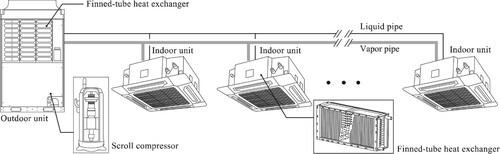
Figure 1 shows a typical VRF system modelled in this study. The proposed model comprises multiple indoor units connected to a single outdoor unit. Both the outdoor and indoor units use a finned-tube heat exchanger. The input energy is supplied from electricity or gas (engine). The energy is used to power the scroll compressor inside the outdoor unit. The outdoor and indoor units are connected by liquid and vapour pipes; i.e. no heat recovery is performed between the indoor units. Both the indoor and outdoor units have expansion valves; however, these valves are not modelled and assumed to be ideally controlled for pressure reduction. The accumulator is not modelled and the amount of refrigerant charged is not considered a parameter because the aim is to simulate annual energy and not reproduce the dynamic characteristics within seconds.

Figure 1 Typical VRF system modelled in this study. (Modified from figures presented in SHASE (2010)).

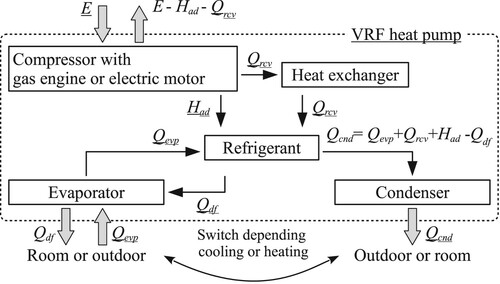
The energy flow of the VRF heat pump model to be developed in this study is shown in Figure 2. The compressor is driven by a gas engine or an electric motor, and the energy, E [kW], is supplied from outside the system in the form of gas or electricity. Part of this energy is converted to the compression head (H_ad [kW]), the part is recovered as waste heat (Q_rcv [kW]), and the remainder is dissipated outside the system. The evaporator and condenser exchanges heat with the moist air (Q_evp [kW] and Q_cnd [kW]). In case of frosting, Q_df [kW] must be dissipated outside the system for defrosting. Inside the VRF heat-pump system, energy is exchanged between components (the compressor, heat recovery heat exchanger, evaporator, and condenser) via a refrigerant.

Figure 2 Energy flow of VRF heat pump model.

This paper is organized into six sections in addition to the introduction (Section 1) and discussion (Section 8). Sections 2–5 explain the structure of the model, and Sections 6 and 7 report the results of performance verification and case studies.

Models for the evaporator and condenser are developed in Sections 2 and 3. By solving the heat exchange of these devices through physical equations, these models can be used to predict the impact of changes in the outdoor and indoor temperature and humidity conditions or an unbalanced indoor unit heat load on the refrigerant temperature.

In Sections 4 and 5, the methods to calculate the cooling and heating operations of the VRF pump are explained. Additionally, methods for initializing the parameters based on technical data provided by the manufacturers are described for each operation. While the content of these sections is similar, there are certain phenomena that are unique to each mode of operation, such as water spraying, defrosting, and gas engine heat recovery.

Section 6 presents a comparison of the results measured in this study with those of previous studies. Section 7 reports the results of an annual energy simulation integrated with a building heat load calculation model for a typical office building. It describes the impact of capacity, water spray, pipe length, and heat recovery on the performance of the VRF heat-pump system on an annual basis. The speed of the calculation and the use of the model in design practice are also discussed.

2. Development of the physical model of evaporator

2.1 General description

To evaluate the thermal environment in a room, it is necessary to be able to predict the ratio of sensible heat to latent heat. In addition, the defrost load must be predictable to express the low-efficiency operation in the cold winter. For this reason, the evaporator model should be able to represent the mechanism of cooling, condensation, and finally, freezing of the inlet air of the heat exchanger.

The change of the moist air state in the evaporator is shown in Figure 3. Due to the bypass effect, it is assumed that the moist air is cooled and dehumidified with constant relative humidity, after ϕ_wp [%] is reached. For this reason, it is assumed that the condensation begins at a temperature slightly higher than the dew point. In the following, this point is referred to as the wet point. When the dry-bulb temperature falls below 0 °C, the condensed water freezes. As shown in Figure 3, there are two possible paths of state change, based on the state of the inlet moist air.

Figure 3 Change in moist air state in the evaporator.

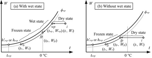
Figure 3(a) represents the case where the wet point is reached before the temperature drops below 0 °C. The calculation described in the plots can be categorized into three segments, each corresponding to the dry, wet, and frozen states of the coil. Figure 3(b) shows the case where the wet point is reached after the temperature drops below 0 °C, and the calculations for the dry and frozen state of the coil require to be separated. The dry, wet, and frozen states of the coil are denoted by the subscripts d (dry), w (wet), and f (frozen), respectively, and the points crossing the corresponding segments are denoted by the subscripts wp (wet point) and fp (frozen point), respectively. The inlet and outlet of the air are represented by the subscripts i and o, respectively.

The sum of the heat flows corresponding to the three states of the coil, as shown in Eq. 1, is the heat flow of the entire evaporator Q_evp [kW], and the basic equations for each area need to be simultaneously solved. (1) $Q_{evp}=Q_d+Q_w+Q_f$(1)

2.2 Basic formulae

1) Heat flow in dry coil

The basic formula for heat flow in the dry state of the coil is as follows: (2) $\begin{array}{rl}{Q}_d& =m{c}_{ma}(t_{ma,i}-t_{ma,wp})\end{array}$(2) (3) $\begin{array}{rl}{Q}_d& ={\epsilon }_{d}m{c}_{ma}(t_{ma,i}-t_{r,evp})\end{array}$(3) Eq. 2 represents the heat flow caused by the temperature difference between the inlet and outlet of the moist air, where t_ma [°C] indicates the temperature of the moist air, and mc_ma [kW/K] denotes the heat capacity flow rate of the moist air. Eq. 3 represents the heat flow based on the effectiveness ϵ_d [-], where t_r,evp [°C] denotes the evaporation temperature of the refrigerant. Assuming that the evaporation temperature is constant, ϵ_d can be calculated by the following formula (Kays and London 1984): (4) ${\epsilon }_d=1-exp\left(-\frac{K_d{S}_d}{m{c}_{ma}}\right)$(4) where K_d [kW/(m²·K)] and S_d [m²] represent the overall heat transfer coefficient and heat transfer area of the dry state coil, respectively. K_d is assumed to be a fixed value and is obtained from the following equation (Inoue 2008): (5) $\frac{1}{K_d}=\frac{R_{r-ma}}{{\alpha }_r}+\frac{1}{{\eta }_F{\alpha }_{ma}}$(5) where R_r-ma [-] denotes the surface area ratio of the air side to the refrigerant side, α_r [kW/(m²·K)] and α_ma [kW/(m²·K)] represent the heat transfer coefficients of the refrigerant and air sides, respectively, and η_F [-] denotes the fin efficiency. The values were set to 15, 6, 0.1, and 0.9, respectively, which refers to the previous studies (JSRAE 2006; Ozeki et al. 2001; Ishibashi and Matsuda 2017; Shibata 2007). K_d was calculated as 0.074.

Strictly speaking, the value of K_d varies with the velocity of the fluid, the temperature, and the shape of the fins. Research has been conducted to predict the variation of K_d precisely for improving the performance of heat exchangers. However, the value of K_d was fixed to minimize the number of parameters because the aim of this study is developing a model that can be initialized automatically from technical data. If a method to adjust the value of K_d based on flow velocity and other factors automatically is established, it should be introduced for improving the prediction performance of the model.

Refrigerant vapour is superheated following the heat exchange in the evaporator; therefore, the temperature is not constant. However, in a typical heat pump cycle, because the heat exchange in the temperature-changing region is less than 10% of the total heat exchange, ignoring the temperature change will not produce a large error. Ignoring the temperature change eliminates the need to calculate the refrigerant flow rate in the evaporator model that reduces the loop for convergence calculation and significantly improves the calculation speed.

2) Heat flow in wet coil

The basic formula for heat flow in a wet coil is as follows. (6) $\begin{array}{rl}{Q}_w& =m_{ma}(h_{wp}-h_{fp})\end{array}$(6) (7) $\begin{array}{rl}{Q}_w& ={\epsilon }_w{m}_{ma}(h_{wp}-h_{sat,evp})\end{array}$(7) Eq. 6 represents the heat flow calculated from the difference in the inlet and outlet specific enthalpies of the moist air, where h_ma [kJ/kg] and m_ma [kg/s] are the specific enthalpy and mass flow rate of the moist air, respectively. Eq. 7 is the heat flow based on the effectiveness, ϵ_w, calculated based on the following formula. (8) ${\epsilon }_w=1-\exp \left(-\frac{K_w{S}_w}{m_{ma}}\right)$(8) h_sat,evp [kJ/kg] denotes the specific enthalpy of the saturated air at the refrigerant temperature (t_r,evp), and it is calculated by the following formula (ASHRAE 1997). (9) $h_{sat,evp}=c_{p,a}{t}_{r,evp}+({\gamma }_{v0}+c_{p,v}{t}_{r,evp})W_{sat,evp}$(9) Here, c_p,a (=1.006 kJ/(kg·K)) denotes the isobaric specific heat of dry air, γ_v0 (=2,501 kJ/kg) denotes the evaporative latent heat of water at 0 °C, c_p,v (=1.805 kJ/(kg·K)) denotes the isobaric specific heat of water vapour, and W_sat,evp [kg/kg] denotes the saturated absolute humidity at t_r,evp.

The overall heat transfer coefficient, K_w, was calculated using the following formula based on the heat- and mass-transfer analogy (ASHRAE 1997). (10) $K_w=\frac{K_d}{c_{p,a}+c_{p,v}W}=\frac{K_d}{c_{p,ma}}$(10) The average of the values at the wet point and the frozen point is used because c_p,ma [kJ/(kg·K)] denotes the isobaric specific heat of moist air and its value varies with absolute humidity; this is shown in Eq. 11. (11) $c_{p,ma,w}=0.5(c_{p,ma,wp}+c_{p,ma,fp}).$(11)

3) Heat flow in frozen coil

The basic formula for heat flow in a frozen coil is as follows. (12) $\begin{array}{rl}{Q}_f& =m_a(h_{fp}-h_o)\end{array}$(12) (13) $\begin{array}{rl}{Q}_f& ={\epsilon }_f{m}_a(h_{fp}-h_{sat,evp})\end{array}$(13) Because frost reduces the heat transfer performance of the fins, the effectiveness, ϵ_f, is calculated by introducing a correction factor, C_f, as shown in Eq. 14. (14) ${\epsilon }_f=1-\exp \left(-\frac{C_f{K}_w{S}_f}{m_a}\right)$(14) A detailed calculation method has been proposed by Aoki, Hattori, and Itoh (1985) for the effect of frost on the heat transfer coefficient; however, it requires information on the fin pitch and pipe size, and this information is not readily available to the HVAC designers. Back-calculating from the study conducted by Aoki, Hattori, and Itoh (1985), the value of C_f is 0.5–0.6, under the condition that the thickness of the frost is 1 mm and the velocity in the evaporator is approximately 5–15 m/s. Therefore, in the model of this study, C_f is constant at 0.6. The overall heat transfer coefficient, K_w, is calculated in Eq. 10, similar to the case of the wet state of the coil, although the specific heat of the moist air at the frozen point is substituted for c_p,ma.

The water that has frosted on the fins must be heated to 0 °C to melt it, and the heat load (Q_df) required for this defrosting is calculated as follows. (15) $Q_{df}=m_a({\gamma }_{s0}-c_{p,ic}{t}_o)(W_{fp}-W_o)$(15) Here, γ_s0 ( = 2,837 kJ/kg) denotes the latent heat of sublimation of ice at 0 °C and c_p,ic ( = 2.09 kJ/(kg-K)) denotes the isobaric specific heat of ice.

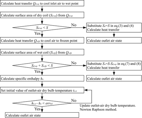
2.3 Numerical solution to basic formulae

For the simulation of the heat pump cycle (details will be described in Sections 4 and 5), three calculations are required: 1) estimation of the heat transfer area (S_evp) from the nominal conditions, 2) determination of the heat flow (Q_evp) from the evaporation temperature (t_r,evp) of the refrigerant, and 3) determination of the required evaporation temperature (t_r,evp) from the heat flow (Q_evp). These are detailed below.

1) Estimation of heat-transfer area (S_evp)

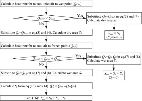
The procedure for calculating the heat transfer area based on the nominal conditions (evaporation temperature, heat flow, air temperature, air humidity, and air flow rate), is shown in Figure 4. First, the heat flow required to cool the moist air down to the wet point (Q_d,wp [kW]), is calculated. If Q_d,wp exceeds the nominal cooling capacity, Q_evp,N, it implies the completion of the heat exchange in the dry state of the coil, such that the heat transfer area, S_evp, is directly calculated by substituting Q_evp,N for Q_d in Eq. 3 and Eq. 4. If the Q_d,wp value is smaller than the Q_evp,N, value, Q_d,wp is substituted for Q_d, to obtain the heat transfer area, S_d, in the dry state of the coil. By repeating the same calculation for the wet and frozen state of the coil, the heat transfer area for each area can be obtained. By adding these areas, the heat transfer area of the entire evaporator can be estimated.

Figure 4 Flowchart of heat-transfer surface (S_evp) calculation.

2) Calculation of heat flow (Q_evp)

The procedure for calculating the heat flow using the refrigerant evaporation temperature, t_r,evp, is shown in Figure 5. Similar to the estimation of the heat transfer area, it is calculated in the order of dry, wet, and frozen state of the coil, to estimate the state of the outlet air.

Figure 5 Flowchart of heat transfer (Q_evp) calculation.

If the evaporator is used in an outdoor unit and frost occurs, Q_df of heat must eventually be supplied to melt it. Therefore, the net heat that can be obtained from the outdoor air using the evaporator is, on average, (Q_evp – Q_df), rather than Q_evp. Whether the model should calculate Q_evp or (Q_evp – Q_df), depends on the situation. The method for making this distinction is explained in Section 5, where the development of VRF model for the heating mode, is discussed.

3) Calculation of evaporation temperature (t_r,evp)

Assuming an initial value of the evaporation temperature, the heat flow is calculated using the method explained in 2) above, and the convergence calculation is performed using the Newton–Raphson method such that this becomes the target value. The same method can be used when the outlet air setpoint temperature is provided as an input, instead of the heat flow.

2.4 Sensitivity analysis

The developed evaporator model was used to analyze the sensitivity of the inlet air to the temperature, humidity, and load. The nominal specifications of the evaporator are listed in Table 1. The calculation results are shown in Figure 6.

Figure 6 Result of the sensitivity analysis of the evaporator model.

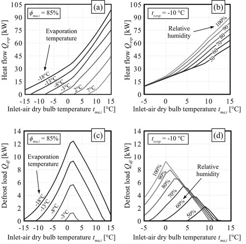
Table 1 Nominal specifications of the evaporator.

Evaporation temperature, tr,evp	2 °C
Heat exchange, Qevp	13 kW
Inlet-air dry bulb temperature, tma,i	7 °C
Inlet-air relative humidity, ϕma,i	85%
Air flow rate, mma	0.056 kg/s (167 m^3/h)
Constant relative humidity when moist air is cooled by an evaporator, ϕbp	95%

Figure 6(a) and (b) show the relationship between the inlet dry bulb temperature (t_ma,i) and heat flow (Q_evp), and Figure 6(c) and (d) show the relationship between the inlet dry bulb temperature and defrost load (Q_df). Figure 6(a) and (c) show the calculation results for each evaporation temperatures (with inlet relative humidity fixed at 85%) while Figure 6(b) and (d) show the calculation results for each relative humidity (evaporation temperature is fixed at −10 °C).

The higher the inlet dry bulb temperature, the larger is the temperature difference between the refrigerant and the air; therefore, the heat flow assumes a right ascending curve. This trend is the same for the defrost load; however, if the inlet dry bulb temperature is extremely high, the heat for cooling is used before frosting commences, and therefore, the value of the defrost load changes to a downward curve after a certain point. If the relative humidity is small, the sensible heat load is large, and frosting does not occur easily; on the contrary, if the relative humidity is large, frosting occurs rapidly. As a result, the defrost load has a maximum point with respect to the inlet dry bulb temperature, and this point depends on the relative humidity.

It is clear from this figure that the effect of frost varies particularly nonlinearly with the combination of temperature and humidity of the outside air. It is difficult to represent it with a simple performance curve, and it requires the use of a physical model, such as the one proposed in this study.

3. Development of the physical model of condenser

3.1 General description

The calculation is simpler than that in the evaporator model because the moist air does not change the state in the condenser. However, in recent years, water is sprayed on the condenser of outdoor units to improve heat exchange through vaporization (Nakagawa et al. 2011; Yamaguchi et al. 2005; Yamaguchi et al. 2006); therefore, the ability to evaluate this effect may prove beneficial. In this study, the moist air state change with water spray is modelled as shown in Figure 7.

Figure 7 Moist air state change at the condenser.

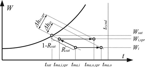
Without water spray, the outdoor air entering the condenser at the dry bulb temperature, t_ma,i, is heated toward the condensation temperature, t_r,cnd [°C], that becomes t_ma,o. When water is sprayed, the air is humidified and cooled, following a constant wet-bulb temperature line to reach t_ma,i,spr, and subsequently, heated to reach t_ma,o,spr. Because the temperature difference between the moist air and refrigerant is larger when water is sprayed, the difference of the inlet/outlet specific enthalpy of the moist air is larger with, than without, water spray (Δh_io [kJ/kg] < Δh_io,spr [kJ/kg]).

3.2 Basic formulae

The following formulae expresses the heat flow, Q_cnd [kW], in the condenser: (16) $\begin{array}{rl}{Q}_{cnd}& =m{c}_{ma}(t_{ma,o}-t_{ma,i})\end{array}$(16) (17) $\begin{array}{rl}{Q}_{cnd}& ={\epsilon }_{cnd}m{c}_{ma}(t_{r,cnd}-t_{ma,i})\end{array}$(17) (18) $\begin{array}{rl}{\epsilon }_{cnd}& =1-\exp \left(-\frac{K_{cnd}{S}_{cnd}}{m{c}_{ma}}\right)\end{array}$(18) where S_cnd [m²] and ϵ_cnd [-] are the heat transfer area and effectiveness of the condenser, respectively. K_cnd [kW/(m²·K)] denotes the overall heat transfer coefficient, and 0.074 kW/(m²·K) is used, similar to that in the dry state coil of the evaporator.

In the case of water spraying, the inlet dry bulb temperature, t_ma,i, of the moist air is replaced by t_ma,i,spr, which is calculated by the following formula, (19) $t_{ma,i,spr}=t_{ma,i}-R_{sat}(t_{ma,i}-t_{sat})$(19) where R_sat [-] denotes the saturation efficiency that indicates the proximity of the inlet air to the saturation temperature, t_sat [°C], by water spray. This value depends on the water spray method; however, according to the actual measurement reports by Nakagawa et al. (2011) and Yamaguchi et al. (2005; 2006), it is approximately 0.4–0.5 for packaged outdoor units and 0.6–0.7 for heat pump chillers. Further, Yamaguchi reported that for the outdoor units of the type that spray water directly onto the fins, almost all sprayed water was evaporated, and based on this result, the water consumption rate m_spr [kg/s] due to water spraying can be calculated using the absolute humidity at the inlet and outlet of the moist air by (20) $m_{spr}=m_{ma}(W_{i,spr}-W_i)=m_{ma}{R}_{sat}(W_{sat}-W_i)$(20)

3.3 Numerical solution of basic formulae

Similar to the case of the evaporator model, it is necessary to 1) estimate the heat transfer area (S_cnd) from the nominal conditions, 2) calculate the heat flow (Q_cnd) from the refrigerant condensation temperature (t_r,cnd), and 3) calculate the required condensation temperature (t_r,cnd) from the heat flow (Q_cnd). However, unlike the evaporator model, all of these three calculations can be solved analytically from Eqs.16–18 without iterative calculations.

3.4 Sensitivity analysis

The developed condenser model was used to analyze its sensitivity to the air temperature, humidity and water spray. The nominal specifications of the condenser are listed in Table 2. The calculation results are shown in Figure 8.

Table 2 Nominal specifications of the condenser.

Condensation temperature, tr,cnd	45 °C
Heat exchange, Qcnd	25 kW
Inlet-air dry bulb temperature, tma,i	35 °C
Inlet-air relative humidity, ϕma,i	55%
Air flow rate, mma	0.056 kg/s (167 m^3/h)

Figure 8 Result of the sensitivity analysis of the condenser model.

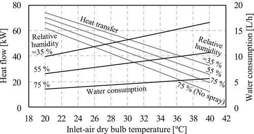
In the case of no water spray, only the result of 75% relative humidity is provided because the heat flow is almost the same, even when the relative humidity changes. As the inlet dry bulb temperature decreases, the heat flow increases due to the larger temperature difference between the air and refrigerant. With water spray, rather than without, the heat flow is larger. Even in the same case of water spray, the lower the relative humidity, the greater is the heat of vaporization, and therefore, the greater is the effect. Further, the water consumption rate by water spray increases with the increase in heat flow.

4. Development of VRF model for cooling mode (refrigeration cycle)

The physical properties of the refrigerant are required to calculate the refrigeration cycle. The remaining values can be computed based on two of the following values: the pressure, specific enthalpy, temperature, density, and specific heat ratio of the refrigerant.

The sample VRF system modelled in this study uses R-410A as the refrigerant, similar to that in many commercial machines. This refrigerant is expected to be replaced by R32 or other natural refrigerants in the future owing to its high global warming potential; however, the calculation procedure remains the same. The fast calculation library developed for annual energy calculation by Togashi (2014) is used in this study because calculating the thermodynamic properties of refrigerants is time consuming. It takes only 1/3 of the computation time of REFPROP version 7 when using this library for R-410A; further, the error with REFPROP is less than 1%.

4.1 Basic formulae

The compression head, H_ad [kW], of the compressor is calculated by multiplying the supplied energy, E [kW], by the compression head efficiency, Eff_hd [-], as following equation. (21) $H_{ad}=E\cdot Ef{f}_{hd}$(21) The compression head efficiency, Eff_hd, is calculated by multiplying the efficiency at 100% load (Eff_hd,100 [-]) by the compression efficiency ratio, R_eff [-], as follows. (22) $Ef{f}_{hd}=Ef{f}_{hd,100}\cdot R_{eff}=Ef{f}_{hd,100}\cdot f(p{l}_{hd})$(22) R_eff denotes a function of the partial load rate, pl_hd [-], and the function is the only performance curve for the model developed in this study.

The partial load rate, pl_hd, is the ratio of the compression head, H_ad, under the relevant condition, to the nominal compression head, H_ad,N [kW], and it is defined in Eq. 23. (23) $p{l}_{hd}=H_{ad}/H_{ad,N}$(23) Further, the compression head can be calculated by following the formula as a function of the compressor inlet and outlet pressures (P_cmp,o [kPa] and P_cmp,i [kPa]), refrigerant volumetric flow rate, v_r [m³/s], and specific heat ratio, κ [-] (ASHRAE 2004). (24) $H_{ad}=\frac{\kappa }{\kappa -1}{P}_{cmp,i}{v}_r\left\{{\left(\frac{P_{cmp,o}}{P_{cmp,i}}\right)}^{\frac{\kappa -1}{\kappa }}-1\right\}$(24) Eq. 24 represents the isentropic process of an ideal gas. Thus, the effects of isentropic and volumetric efficiencies are not included in this equation, but instead in Eq. 22.

The energy exchanged with the refrigerant in the condenser, evaporator, and compressor is expressed by the following formula based on the inlet and outlet specific enthalpy of the refrigerant and the refrigerant mass flow rate (m_r [kg/s]), respectively. (25) $\begin{array}{rl}{Q}_{cnd}& =m_r(h_{r,cnd,i}-h_{r,cnd,o})\end{array}$(25) (26) $\begin{array}{rl}{Q}_{evp}& =m_r(h_{r,evp,o}-h_{r,evp,i})\end{array}$(26) (27) $\begin{array}{rl}{H}_{ad}& =m_r(h_{r,cnd,i}-h_{r,evp,o})\end{array}$(27)

In the case of a heat pump using a gas engine, part of the input energy is recovered and used for heating (Q_rcv). When the outdoor unit is frosted, it is necessary to supply heat (Q_df) for defrosting. Consequently, the energy balance between the condenser, evaporator, and compressor by the refrigerant is expressed in the following equation. (28) $0=H_{ad}+Q_{evp}-Q_{cnd}+Q_{rcv}-Q_{df}$(28)

4.2 Coupled calculation method of basic formulae

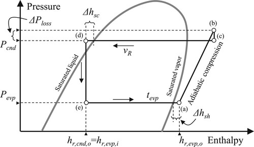
The refrigeration cycle assumed in this model is shown in Figure 9.

Figure 9 Refrigeration cycle.

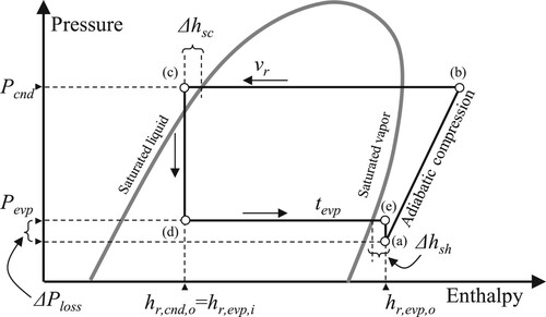
After adiabatic compressive heating by the compressor (a→b), the refrigerant is cooled in the condenser inside the outdoor unit (b→c) and sent to the indoor unit in a sub-cooled state (c→d). After being heated in the evaporator inside the indoor unit (d→e), ΔP_loss [kPa] of pressure is lost during transport that eventually returns to the compressor (e→a).

Table 3 summarizes the boundary conditions of the VRF heat pump model. The inputs are conditions that can be changed during the simulation, and the parameters are conditions that are constant throughout the simulation.

Table 3 Boundary conditions of the VRF heat pump model.

Inputs	Indoor-unit outlet-air setpoint temperature, air flow rate of indoor units, Indoor air state, outdoor air state, indoor-unit outlet-air setpoint humidity ratio (required only while calculating the heating operation.)
Parameters	Nominal compression head, pipe resistance coefficient, super-heat degree, sub-cool degree

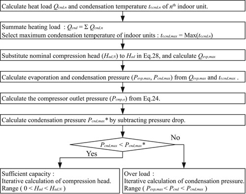
The outline of the calculation procedure of the cooling model is shown in Figure 10. When the load is less than the cooling capacity of the machine, the compression head should be lowered; conversely, when the machine is overloaded, the evaporation pressure should be increased. Therefore, depending on whether the machine is overloaded or not, the unknown variable for convergence calculation is switched to either the compression head or the evaporation temperature. The detailed calculation procedure is explained below.

Figure 10 Outline of the calculation procedure of the cooling model.

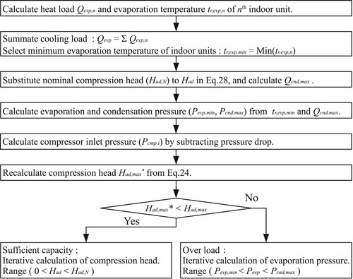
1) Calculation of evaporation temperature and pressure

The evaporator model developed in Section 2 is used to calculate the required evaporation temperature (t_r,evp,n [°C]) from the outlet air setpoint temperature of each indoor unit. The VRF heat pump system must realize the refrigeration cycle at the lowest temperature (t_r,evp,min [°C]). Furthermore, the total heat load (Q_evp,n) of all the N_I indoor units is added, as shown in Eq. 29. (29) $Q_{evp}=\sum _{n=0}^{N_I}{Q}_{evp,n}$(29) The evaporation temperature should be increased as much as possible to improve the efficiency of the VRF heat pump system, although there are systems where the temperature cannot be controlled. In this case, the temperature is fixed at the nominal value. Even for systems that can control the evaporation temperature, in reality, the temperature cannot be increased without limit; therefore, a lower limit for the compression ratio, R_HL [-] (=P_cnd/P_evp), is set. In this model, the lower limit (R_HL,min [-]) is set at 1.5, referring to the report by Honda and Sano (1999).

2) Calculation of refrigerant volumetric flow rate

To determine whether the machine is overloaded or not, the refrigeration cycle is first calculated assuming that the compression head is at its maximum value (H_ad,N [kW]). The maximum heat release from the condenser (Q_cnd,max) is obtained by substituting Q_evp and H_ad,N in Eq. 28. Note that Q_rcv and Q_df are both zero because this is a cooling operation.

The required condensation temperature and pressure (t_r,cnd,max [°C], P_cnd,max [kPa]) are calculated from the maximum heat release (Q_cnd,max) using the condenser model. By calculating the refrigerant temperature at the intersection of the condensation pressure and the saturated liquid line and subtracting the sub-cooling degree (Δt_r,sc [°C]), the refrigerant state at the outlet of the condenser can be obtained. As shown in Figure 9, it is considered that the specific enthalpy of the condenser outlet and the evaporator inlet (h_r,cnd,o [kJ/kg] and h_r,evp,i [kJ/kg]) assume the same value.

By calculating the refrigerant temperature at the intersection of the evaporation pressure and the saturated vapour line and adding the superheat degree (Δt_r,sh [°C]), the specific enthalpy of the evaporator outlet refrigerant (h_r,evp,o [kJ/kg]) can be obtained.

Substituting the specific enthalpy at the refrigerant inlet and outlet of the evaporator (h_r,evp,i and h_r,evp,o) in Eq. 26, the mass flow rate of the refrigerant (m_r [kg/s]) is calculated. The mass flow rate (m_r) can be converted to volumetric flow rate (v_r,evp,o [m³/s]), by substituting the refrigerant density (ρ_r,evp,o [kg/m³]) in the following formula. (30) $m_r=v_r\cdot {\rho }_r$(30) The volumetric flow rate (v_r,evp,o) is used to calculate the pressure drop in the piping back to the compressor.

3) Iterative calculation method

The pressure drop in the pipe (ΔP_loss) is the sum of the friction loss (ΔP_loss,p [kPa]) and gravity (ΔP_loss,g [kPa]), as shown in the following equation. (31) $\mathrm{\Delta }{P}_{loss}=\mathrm{\Delta }{P}_{loss,p}+\mathrm{\Delta }{P}_{loss,g}$(31) The friction loss in the pipe is expressed by the following formula (ASHRAE 1997): (32) $\mathrm{\Delta }{P}_{loss,p}=500\lambda \frac{L}{D}{\rho }_r{\left(\frac{v_r}{A}\right)}^2=k_{loss}L{m}_r{v}_r$(32) where λ [-] is the friction coefficient, L [m] is the length, D [m] is the diameter, and A [m²] is the cross-sectional area of the pipe. In this model, by assuming 500λ/(A²D) to be constant as shown in the third term of Eq. 32, the friction loss is calculated simply using the resistance coefficient (k_loss [m⁻¹]).

The pressure change due to gravity is represented by the acceleration of gravity (g [m/s²]) and the height of the outdoor unit (H [m]) with respect to the height of the indoor unit, as shown in the following equation (ASHRAE 1997). (33) $\mathrm{\Delta }{P}_{loss,g}=\{\begin{array}{ll}0.001Hg{\rho }_r& (coolingmode)\\ -0.001Hg{\rho }_r& (heatingmode)\end{array}$(33) It should be noted that in Eq. 33, the sign is reversed for the cooling mode and heating mode because depending on the mode of operation and the vertical relationship between the outdoor and indoor units, the gravity may increase and the VRF capacity may decrease.

Using Eq. 31–34, the pressure difference (ΔP_loss) is calculated from the refrigerant density, flow rate, and height differences, and the difference is subtracted from the evaporation pressure to obtain the compressor inlet pressure. The volumetric flow rate (v_r,cmp,i) is calculated from the refrigerant density (ρ_cmp,i) and mass flow rate (m_r) at the compressor inlet using Eq. 30, and it is substituted into Eq. 24 to obtain the latest compression head (H_ad,max*) value.

If this H_ad,max* is smaller than the maximum compression head assumed at the beginning (H_ad,N), then the cooling load is small. Therefore, the value of the compression head in the range of 0–H_ad,N should be iteratively calculated. If H_ad,max* is greater than H_ad,N, the machine is overloaded. Therefore, the evaporation pressure in the range of P_evp,min – P_cnd,max should be iteratively calculated. Because there is only one state variable, it can be solved using the Brent method (William et al. 2007) that is a root-finding algorithm.

4) Calculation of thermo off ratio

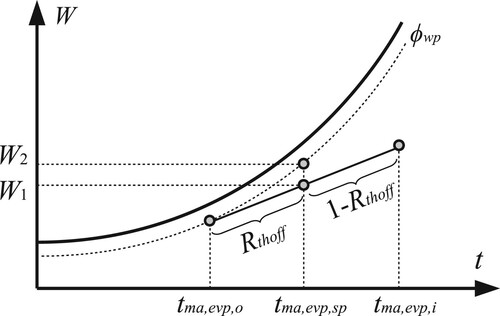
Because the evaporation temperature of the system is set to the temperature required by the indoor unit with the highest partial load rate, if the other indoor units operate at this evaporation temperature, the outlet-air temperature (t_ma,evp,o,n [°C]) will be lower than the set point (t_ma,evp,sp,n [°C]). For this reason, it is assumed that these indoor units are operated at thermo-off for a certain time ratio (R_thoff [-]). R_thoff is calculated by the following equation. (34) $R_{thoff}=1-\frac{t_{ma,evp,i,n}-t_{ma,evp,sp,n}}{t_{ma,evp,i,n}-t_{ma,evp,o,n}}$(34) Figure 11 shows the calculation of the average outlet-air state based on the thermo-off time ratio. The average outlet-air temperature and humidity (t_{ma,evp,o,ave,n} [°C] and W_{ma,evp,o,ave,n} [kg/kg]) can be calculated using the following equations. (35) $\begin{array}{rl}{t}_{ma,evp,o,ave,n}& =R_{thoff}{t}_{ma,evp,i,n}+(1-R_{thoff})t_{ma,evp,o,n}\end{array}$(35) (36) $\begin{array}{rl}{W}_{ma,evp,o,ave,n}& =R_{thoff}{W}_{ma,evp,i,n}+(1-R_{thoff})W_{ma,evp,o,n}\end{array}$(36) When averaged over time, the outlet-air temperature (t_{ma,evp,o,ave,n}) matches the setpoint temperature (t_ma,evp,sp,n). In Figure 11, the average outlet humidity is W₁. Note that if there had been only one indoor unit and the evaporation temperature could be raised sufficiently, then the average outlet humidity would be W₂. In other words, the air supply air humidity of a VRF heat pump system varies significantly, depending on whether lower evaporation temperatures are required by the other indoor units. The proposed model can reproduce this mutual influence among indoor units.

Figure 11 Calculation of the average outlet air state based on the thermo-off time ratio.

4.3 Method for estimating parameters from nominal performance

In general, the information sources available to HVAC designers are the manufacturer catalogs and technical documents; therefore, it is not possible to obtain detailed information on the internal components of the individual machine. Therefore, a method is developed to estimate the parameters of the model from the information that is readily available to HVAC designers. In the following, a system with two 14.0 kW indoor units connected to a 28.0 kW outdoor unit will be used as an example.

1) Basic information and assumptions

Table 4 summarizes the information used to estimate the parameters of the cooling model.

Table 4 Information used to estimate the parameters of the cooling model.

	Conditions		JIS	Example
Outdoor unit	Cooling capacity	JIS nominal condition (Qevp,N)	x	28.0	kW
		JIS mid-load condition	x	12.6	kW
		JIS mid-load and mid-temperature condition	x	13.2	kW
	Electricity	JIS nominal condition (EN)	x	8.93	kW
		JIS mid-load condition	x	2.35	kW
		JIS mid-load and mid-temperature condition	x	1.94	kW
	Volumetric air flow rate		x	187	m^3/min
	Super-heat degree			1	°C
	Minimum controllable partial load rate (plhd,min)			15	%
Indoor unit	Nominal capacity		x	14.0	kW
	Volumetric air flow rate		x	34.5	m^3/min
	Nominal evaporation temperature			10	°C
	Sub-cool degree			1	°C
Pipe	Nominal length		x	7.5	m
	Capacity correction factor when the length is 100 m (Rpc)			0.88

The ‘JIS’ column in Table 4 indicates whether the information is required by the JIS. Therefore, the checked information is available for the product of any manufacturer. In Table 4, the values of Manufacturer A are provided as examples. The heat load, inlet air temperature, and humidity conditions for the outdoor and indoor units are specified by the JIS. ‘Mid-load’ is defined as the load at 50% of the rated capacity. The inlet air state of the outdoor unit is 35 °CDB/24 °CWB for the nominal and mid-load conditions, 29 °CDB/19 °CWB for the mid-load, mid-temperature condition, and that of the indoor unit is 27 °CDB/19 °CWB for all conditions (JIS 2015a; 2015b; 2015c).

The manufacturer documents present a table of correction factors for the extent of variation of the capacity of the evaporator with respect to the nominal capacity, depending on the pipe length. Further, the lower limit of the controllable partial load rate is disclosed.

However, the nominal super-heating degree, sub-cooling degree, condensation temperature, and evaporation temperature are not specified by the JIS and are assumed. In this model, both the super-heat and sub-cooling degrees were set to 1 °C. Because these values are not predicated on anything specific, they can even be set to 0 °C. However, in preparation for future improvements, the model is made capable of setting non-zero values.

In actual machines, sub-cooling and super-heating degrees are controlled to stabilize the refrigeration cycle, and they are not always constant. It is better to model such control to make the model closer to reality; however, in such a case, the numerical calculation becomes unstable. Therefore, two issues remain for the future of this model: 1) what should be the values of these temperatures, and 2) how they should be controlled.

The evaporation temperature of the indoor unit is in the control range of 3–13 °C, in the model proposed by Zhou et al. (2008). In this model, the manufacturer participated in the development; therefore, the values are highly reliable.

Figure 12 shows the results of calculating the nominal outlet-air temperature for 10 different indoor units of Manufacturer A using the information in the technical documents. Even if several different indoor units are connected to the same outdoor unit, each indoor unit must be able to perform at its nominal capacity. Therefore, the evaporation temperature can be expected to be lower than 11.4 °C, the minimum value in Figure 12.

Figure 12 Cooling capacity and nominal outlet-air temperature for 10 different indoor units.

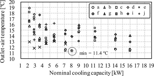
Considering the above, the nominal evaporation temperature was set to 10 °C in the model of this study.

The nominal condensation temperature of outdoor units may have different values for different models. In general, manufacturers sell models with the same body size and different cooling capacities. It can be assumed that the models with a higher cooling capacity have a higher nominal condensation temperature because they are forced to have smaller airflow and heat transfer area per capacity, than the other models with the same body size. To verify the presence of such a tendency, the index, R_qma,c [kw/(kg/s)], was introduced. R_qma,c is the cooling capacity per air flow rate of the outdoor unit, as defined by the following equation. (37) $R_{qma,c}=Q_{evp,N}/m_{ma,N}$(37) Figure 13 (adopted from the technical documentations of six major Japanese companies) depicts the relationship between R_qma,c, COP, and outlet air temperature is shown in Figure 13. This figure was adopted from the technical documents of six major Japanese companies.

Figure 13 Relationship between R_qma,c, COP, and outlet-air temperature.

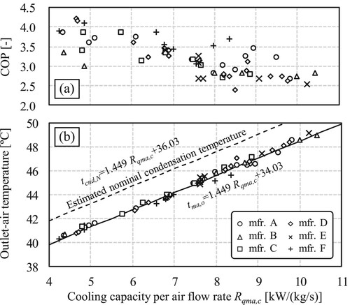
As R_qma,c increases (i.e. the air flow rate per cooling capacity decreases), COP tends to decrease (Figure 13(a)). This can be attributed to the increase in the compression ratio at the high condensation temperatures. Figure 13(b) shows the result of estimating the outlet air temperature of the outdoor unit by substituting the JIS outdoor air condition and the nominal condition in the following equation. (38) $t_{ma,cnd,o}=t_{ma,cnd,i}+\frac{Q_{evp}+E}{c_{pma}{m}_{ma,cnd}}$(38) In the model of this study, the approach of the condensation temperature and the outlet-air temperature of the outdoor unit was assumed 2 °C, and the nominal condensation temperature was estimated by the following equation. (39) $t_{r,cnd,N}=1.449R_{qma,c}+36.03$(39)

2) Estimation of heat transfer area of indoor units

Because the heat flow, inlet air conditions, and evaporation temperature can be specified based on Table 4 and the JIS conditions, the heat transfer area of the evaporator (S_evp) can be estimated by the evaporator model developed in Section 2.

3) Estimation of compression head and resistance coefficient

The resistance coefficient (k_loss) in Eq. 32 can be derived using a dimensionless number obtained from the thermal conductivity and viscosity coefficient of the refrigerant. However, the calculation speed decreases due to the need to calculate the physical properties of the refrigerant, and the modelling work increases because the average pipe diameter of the entire VRF heat pump system is required. Therefore, a simple method of estimating the resistance coefficient (k_loss) from the pipe length correction factor (R_pc [-]) in the technical data, has been developed.

R_pc is a correction factor used for estimating the cooling capacity of the VRF system at the relevant pipe length (Q_evp,pc [kW]) by multiplying the nominal cooling capacity (Q_evp,N) as shown in the following equation. (40) $Q_{evp,pc}=R_{pc}{Q}_{evp,N}$(40) Figure 14 shows the change in the refrigeration cycle when the piping length increases. The condensation and evaporation temperatures, after the change can be easily approximated using R_pc, as explained below.

Figure 14 Refrigeration cycle changes with long refrigerant piping.

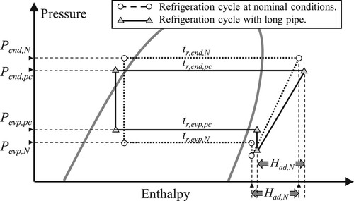
If the coil states are not divided into dry, wet, and frozen, the heat flow at the evaporator can be simply expressed by the following formula. (41) $Q_{evp}=\epsilon m{c}_{ma}(t_{ma,i}-t_{r,evp})$(41) t_ma,i, mc_ma, and ϵ do not change when the pipe length changes. Therefore, by combining Eq. 40 and Eq. 41, the evaporation temperature (t_r,evp,pc [°C]) after the pipe-length correction can be expressed by the following equation using R_pc. (42) $t_{r,evp,pc}=(1-R_{pc})t_{ma,evp,i}+R_{pc}{t}_{r,evp,N}$(42) This indicates that the evaporation temperature approaches the indoor unit inlet air temperature as R_pc increases. In other words, as the pipe length increases, the evaporation pressure increases, as shown in Figure 14.

As shown in the following equation, the heat flow in the condenser is assumed to change at the same rate as that in the evaporator when the pipe length changes. (43) $Q_{cnd,pc}\approx R_{pc}{Q}_{cnd,N}$(43) Combining Eq. 43 with Eq. 41, the condensation temperature (t_r,cnd,pc [°C]) after the pipe-length correction, can be approximated by the following equation. As the pipe length increases, the condensation temperature approaches the outdoor-air temperature, and the pressure decreases. (44) $t_{r,cnd,pc}=(1-R_{pc})t_{ma,cnd,i}+R_{pc}{t}_{r,cnd,N}$(44) The above resulted in two different combinations of condensation and evaporation pressures one with and the other without the pipe length correction. The resistance coefficient (k_loss) is calculated iteratively such that the compression head (H_ad,N) value is the same for these two combinations. Substituting this compression head (H_ad,N) into Eq. 21, the compression head efficiency (Eff_had,100) at the nominal conditions can be obtained.

4) Estimation of heat transfer area of outdoor unit

Substituting the nominal compression head (H_ad,N) into Eq. 28, the heat release (Q_cnd,N) at the condenser can be calculated, and by setting the JIS outdoor air condition and Q_cnd,N to the condenser model, the heat transfer area (S_cnd) of the condenser can be estimated.

5) Result of parameter estimation

Table 5 lists the cooling model parameters estimated from the values illustrated in Table 4 using the method described above.

Table 5 Estimated parameters of cooling model.

Heat transfer area of indoor unit, Sevp	21.2	m^2
Heat transfer area of outdoor unit, Scnd	69.1	m^2
Pressure drop at nominal pipe length (7.5 m), ΔPp,loss,N	24	kPa
Pressure drop at comparison pipe length (100 m)	244	kPa
Resistance coefficient of pipe, kloss	4018	m^−1
Nominal compression head, Had,N	5.65	kW
Compression head efficiency at full load, Effhad,100	0.63	-

4.4 Estimation of partial load performance curve

Based on the information on mid-load condition and mid-load mid-temperature condition listed in Table 4, the compression head efficiency ratio (R_eff) under a partial load can be estimated as follows.

Because the cooling load of the indoor units is known, the heat release from the condenser (Q_cnd) can be calculated from Eq. 28, assuming an initial value for the compression head (H_ad). Therefore, using the evaporator and condenser models, the evaporation and condensation pressures can be obtained. Using these pressures and the degrees of sub-cooling and super-heat, the inlet and outlet specific enthalpy at the evaporator can be calculated. The mass flow rate of the refrigerant is calculated from the difference in these specific enthalpies using Eq. 26. This is converted to volumetric flow rate using Eq. 30, and subsequently, the pipe pressure drop is calculated using Eq. 32. The above procedure affords the inlet pressure of the compressor, and the latest value of the compression head can be obtained using Eq. 24. The compression head is updated to converge, such that the difference between this value and the initial assumed value becomes sufficiently small.

Because the mid-load condition and mid-load mid-temperature condition feature almost half the cooling capacity of the nominal condition, the Brent method with the range set to 0.1H_ad,N – 0.8H_ad,N should provide the solution.

Figure 15 shows the estimated performance curve of the compression head efficiency ratio.

Figure 15 Estimated performance curve of the compression head-efficiency ratio.

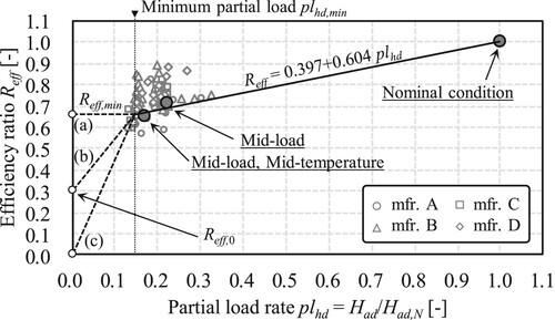
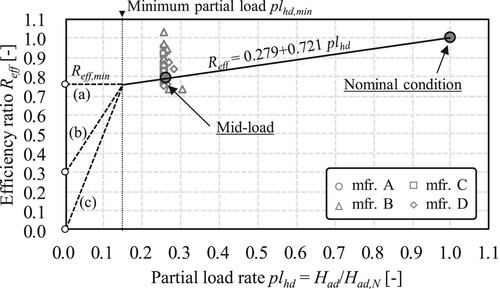
Based on the definition of Eq. 21, the compression head efficiency ratio (R_eff) is 1.0 at 100% load (pl_hd = 1.0). The large circle plot in the figure shows the estimated results for the VRF heat pump in Table 4. In this model, the compression head efficiency ratio (R_eff) is expressed by the linear equation of the partial load ratio (pl_hd), as shown in the figure. For reference, the estimated results for the other VRF heat pumps of four major Japanese manufacturers are also shown. Although the plots are clustered, they are different from each other. Therefore, the coefficients in the characteristic equation should be estimated for each VRF heat pump.

In this model, the machine is assumed to follow this characteristic up to the lower limit of the capacity control. Below the lower limit, because the machine intermittently turned on and off repeatedly (referred to as ‘on/off state’ in the following), the efficiency ratio, in this case, cannot be quantified accurately without a dynamic model.

As shown in the Line (a) in Figure 15, the efficiency ratio at the lower limit can be extended horizontally if the on/off state can be performed without any loss at all. However, in general, such performance cannot be achieved. Assuming the loss caused by the on/off state is the largest, the line should be extended to the origin as shown for Line (c). As shown in Line (b), the moderate characteristic through the intercept between R_eff,min and the origin can be expressed by Eq. 45. The model of this study uses Eq. 45 with R_eff,0 = 0.05. (45) $R_{eff}=\frac{p{l}_{hd}}{p{l}_{hd,min}}{R}_{eff,min}+\left(1-\frac{p{l}_{hd}}{p{l}_{hd,min}}\right)R_{eff,0}$(45)

4.5 Sensitivity analysis of heating model

A sensitivity analysis was performed using a model initialized based on the specifications in Table 4.

1) Sensitivity to cooling load

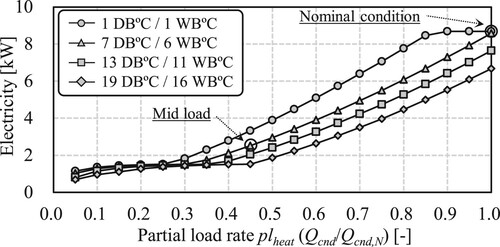
Figure 16 shows the electricity under partial load operation for each outdoor air condition. The partial load rate, pl_heat [-], is defined as the ratio of the actual heat, Q_evp (Q_cnd for heating), to the nominal capacity, Q_evp,N (Q_cnd,N for heating), as shown in the following equation. (46) $p{l}_{heat}=\{\begin{array}{cc}{Q}_{evp}/Q_{evp,N}& (\text{cooling mode})\\ Q_{cnd}/Q_{cnd,N}& (\text{heating mode})\end{array}$(46) Eq. 46 is more commonly used compared to Eq. 23 because the compression head for an actual building cannot be measured directly.

Figure 16 Electricity under partial load operation.

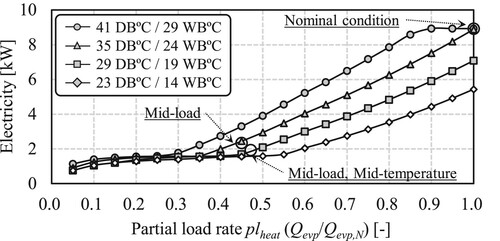
The partial load rate on the horizontal axis is the value defined in Eq. 46 (similar to that for Figure 17). The second and third lines from the top are the nominal and mid-load mid-temperature conditions of JIS, respectively. The line passes exactly through the three JIS test points.

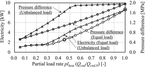
Figure 17 Effect of unbalanced heat load of indoor units on electricity.

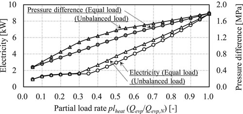
When the inlet temperature of the outdoor unit is low, heat exchange is easier in the condenser, and the compression ratio decreases; therefore, electricity also decreases. The electricity drops as the partial load decreases, although the drop becomes smaller when it reached the lower limit of capacity control. If the outdoor air temperature exceeds that corresponding to nominal conditions, the electricity will reach a head at a partial load rate of approximately 90%. This is an overload situation, and cooling is not possible under this condition.

The effect of unbalanced heat load of indoor units on electricity is shown in Figure 17, where two cases of equal and unbalanced heat load of two indoor units are calculated. In the case of unbalanced heat load, the load of one of the indoor units was preferentially reduced until the partial load rate of the unit reached 5%.

The pressure difference along the vertical axis is the difference between the condensation and evaporation pressures. Compared with the case of equal load, the degree of reduction in electricity is small in the case of unbalanced load. This is because in the case of unbalanced load, the indoor unit on one side has a high heat load and requires a low evaporation temperature; therefore, the differential pressure cannot be lowered.

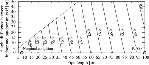
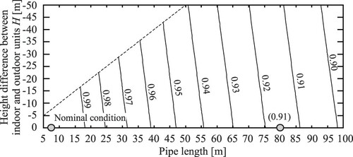
2) Sensitivity to pipe length and installation height of units

Figure 18 shows the relation between the pipe length and height difference between the indoor and outdoor units and the pipe-length correction factor. As listed in Table 4, the correction factor is 0.88 when the pipe length is 100 m; this implies that the calculation result is in accordance with the specifications.

Figure 18 Relationship of pipe length and height difference between indoor and outdoor units and pipe length correction factor.

3) Sensitivity to moist air state of indoor and outdoor units

Figure 19 shows the relationship between the inlet air conditions of the indoor and outdoor units and the COP. Figure 19(a) shows the COP for the combination of inlet dry bulb temperature of the indoor and outdoor units. The COPs for the nominal conditions are almost identical to the specifications listed in Table 4. Because the outdoor air temperature decreases, the condensation pressure also decreases; further, because the indoor air temperature increases, the evaporation pressure also increases, resulting in a smaller value of the compression ratio and an improved COP.

Figure 19 Relationship between the inlet-air conditions of indoor and outdoor units and COP.

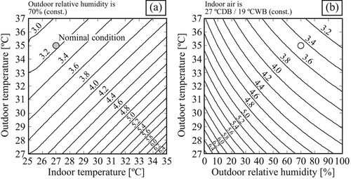
Figure 19(b) shows the COP of the outdoor unit against the combination of dry bulb temperature and relative humidity. Water spraying to the outdoor unit is enabled, and the nominal efficiency is improved by approximately 10%. Because water spraying uses the latent heat of evaporation, the lower the relative humidity, the higher is the COP.

5. Development of VRF model for heating mode (Heat pump cycle)

5.1 Basic formulae

Most of the basic formulae are the same as those in the cooling model; however, the waste heat recovery (Q_rcv) while using a gas engine heat pump (hereafter referred to as GHP), occurs only during the heating model. Heat recovery (Q_rcv) is calculated by multiplying the input energy by the waste heat recovery efficiency (E_ffrcv [-]) using the following equation. (47) $Q_{rcv}=E\cdot Ef{f}_{rcv}$(47) The total efficiency (Eff_ttl [-]) of a gas engine is expressed as the sum of the compression head efficiency (Eff_hd) and the waste heat recovery efficiency (E_ffrcv), as shown in the following equation. (48) $Ef{f}_{ttl}=Ef{f}_{hd}+Ef{f}_{rcv}$(48) Combining Eq. 21, Eq. 47, and Eq. 48, the waste heat recovery can be expressed using the compression head (H_ad) in the following equation. (49) $Q_{rcv}=H_{ad}\frac{Ef{f}_{ttl}-Ef{f}_{hd}}{Ef{f}_{hd}}$(49) If the heat recovery is enabled, a part of the refrigerant (m_r,rcv [kg/s]) is sent to the heat recovery unit, instead of the evaporator, to be heated by the waste heat. The heat exchange at the evaporator and heat recovery unit is calculated by the following equations. (50) $\begin{array}{rl}{Q}_{evp}& =(m_r-m_{r,rcv})(h_{r,evp,o}-h_{r,evp,i})\end{array}$(50) (51) $\begin{array}{rl}{Q}_{rcv}& =m_{r,rcv}(h_{r,evp,o}-h_{r,evp,i})\end{array}$(51) Combining both the equations, the refrigerant flow rate (m_r) can be expressed by the following equation. (52) $m_r=\frac{Q_{evp}+Q_{rcv}}{h_{r,evp,o}-h_{r,evp,i}}$(52)

5.2 Coupled calculation method of basic formulae

The heat pump cycle in this model is shown in Figure 20. The refrigerant that is heated by adiabatic compression (a→b), reaches each indoor unit after losing the pressure of ΔP_loss (b→c). Thereafter, it is cooled in the condenser and returns to the outdoor unit (c→d→e), where it is heated in the evaporator or heat recovery unit and is drawn into the compressor again (e→a).

Figure 20 Heat pump cycle.

The boundary conditions of the model are already listed in Table 3. Note that a setpoint of absolute humidity is added in the heating model because of the humidification.

The calculation procedure for the heating model is shown in Figure 21. When the heating load is small, the heating capacity is reduced by reducing the compression head. In the case of overload, the condensation temperature decreases. Therefore, depending on whether the machine is overloaded or not, the unknown variable for convergence calculation is switched to either the compression head or the condensation temperature.

Figure 21 Calculation procedure for heating model.

1) Calculation of condensation temperature and pressure

The total heat load of each indoor unit is calculated based on the set point of the outlet-air temperature and absolute humidity. The saturation efficiency of the humidifier is assumed to be 100%. In other words, it is assumed that humidification is always possible if there is enough sensible heat.

Using the condenser model, the required condensation temperature and pressure (t_cnd,max, P_cnd,max) can be calculated based on the heat load of each indoor unit. The VRF heat-pump system must realize the heat pump cycle at the highest temperature.

The following equation is used to add the total heat loads of all the indoor units. (53) $Q_{cnd}=\sum _{n=0}^{N_I}{Q}_{cnd,n}$(53)

2) Calculation of refrigerant volumetric flow rate

To determine whether the heat pump cycle is overloaded or not, the calculation is first performed by providing the maximum compression head (H_ad,N [kW]). The maximum load of the evaporator (Q_evp,max) is obtained by substituting Q_cnd and H_ad,N into Eq. 28. If the waste heat from the gas engine can be recovered, Q_rcv (using Eq. 49) must also be substituted into Eq. 28.

The evaporator model is used to determine the required evaporation temperature (t_r,evp,max [°C]) and pressure (P_evp,max [kPa]) based on Q_evp,max. The specific enthalpy difference at the inlet and outlet of the evaporator is calculated based on the degree of superheat and supercooling, and the mass flow rate of the refrigerant is calculated from Eq. 26. Note that in the case of defrosting, (Q_evp,max-Q_df) is used instead of Q_evp,max because the net heat that can be provided to the refrigerant from the evaporator is (Q_evp,max-Q_df).

3) Iterative calculation method

The pressure drop in the pipe (ΔP_loss) is calculated using Eqs. 30–33 in the same procedure as that in the cooling operation. The density of the refrigerant used to calculate the pressure drop in Eq. 32 and Eq. 33 is the density at the inlet of the condenser, rather than the density at the outlet of the compressor. The reason for this is to reduce the number of iterations for the pressure drop, improving the speed and stability of the calculation.

The maximum condensation pressure (P_cnd,max*) can be obtained by substituting the maximum compression head (H_ad,N) into Eq. 24, calculating the compressor outlet pressure, and subtracting the pressure drop in the pipe (ΔP_loss). If this value is lower than the condensation pressure calculated in 1), there is not enough heating capacity, that is, it is overloaded. In the case of overload, the condensation pressure is iteratively calculated in the range of P_evp,max – P_cnd,max. Otherwise, the compression head is iteratively calculated in the range of 0 – H_ad,N.

4) Calculation of thermo off ratio

Similar to the case of the cooling operation, the difference between the setpoint temperature and the actual temperature of the outlet air of the indoor unit is used to calculate the thermo-off time ratio (R_thoff) using Eq. 54. (54) $R_{thoff}=1-\frac{t_{ma,cnd,i,n}-t_{ma,cnd,sp,n}}{t_{ma,cnd,i,n}-t_{ma,cnd,o,n}}$(54)

5.3 Method for estimating parameters from nominal performance

Similar to the cooling operation, a method was developed to estimate the parameters from the manufacturer documents available to the HVAC designer. In the following paragraphs, a system with two 16.0 kW indoor units connected to a 31.5 kW outdoor unit will be discussed as an example.

1) Basic information and assumptions

Table 6 summarizes the information used to estimate the parameters of the heating model. Specific values of the VRF system of Manufacture A are provided as examples. The inlet air conditions for the outdoor and indoor units are the same for the nominal condition and mid-load condition. The indoor unit is 20 °CDB/15 °CWB, and the outdoor unit is 7 °CDB/6 °CWB (JIS 2015a; 2015b; 2015c).

Table 6 Information used to estimate the parameters of the heating model.

-	Conditions		JIS	Example
Outdoor unit	Heating capacity	JIS nominal condition (Qcnd,N)	x	31.5	kW
		JIS mid-load condition	x	14.2	kW
	Electricity	JIS nominal condition (EN)	x	8.68	kW
		JIS mid-load condition	x	2.54	kW
	Volumetric air flow rate		x	187	m^3/min
	Sub-cool degree			1	°C
	Minimum controllable partial load rate (plhd,min)			13	%
Indoor unit	Nominal capacity		x	16.0	kW
	Volumetric air flow rate		x	34.5	m^3/min
	Nominal condensation temperature			46	°C
	Super-heat degree			1	°C
Pipe	Nominal length		x	7.5	m
	Capacity correction factor when the length is 80 m (Rpc)			0.91	−

The condensation temperature of the indoor unit is considered to be in the control range of 42 °C to 46 °C in the model proposed by Zhou et al. (2008).

Figure 22 shows the results of calculating the nominal outlet-air temperature for 10 different indoor units of Manufacturer A using the relevant technical documents. For the same reason as that in the estimation of the evaporation temperature in the cooling model, the nominal condensation temperature can be estimated to be higher than 45.1 °C; this is the maximum temperature shown in Figure 22.

Figure 22 Heating capacity and nominal outlet-air temperatures for 10 different indoor units.

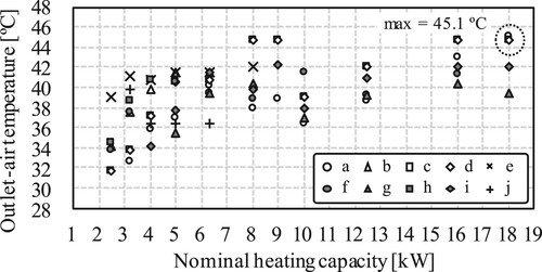
Considering the above, the nominal condensation temperature was set to 46 °C in the model of this study.

The heating capacity per air flow rate of the outdoor unit (R_qma,h [kw/(kg/s)]) is defined by the following equation. (55) $R_{qma,h}=Q_{cnd,N}/m_{ma,N}$(55) The relationship between the R_qma,h, COP, and outlet-air temperature is shown in Figure 23. Similar to the case of cooling, COP decreases as R_qma,h increases (that is, the air flow rate per heating capacity decreases).

Figure 23 Relationship between R_qma,h, COP, and outlet-air temperature.

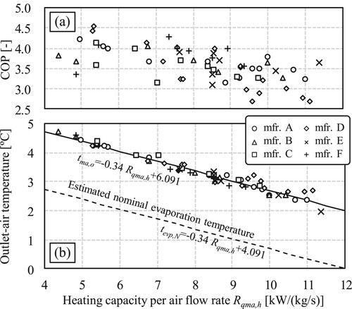
Figure 23(b) shows the result of estimating the outlet-air temperature of the outdoor unit from the nominal conditions using the following equation. (56) $t_{ma,evp,o}=f_{t-h\varphi }\left(h_{ma,evp,i}-\frac{Q_{cnd}-E}{m_{ma,cnd}},{\varphi }_{wp}\right)$(56) where f_t-hϕ(·) is a function to obtain the dry bulb temperature from the specific enthalpy and relative humidity (ASHRAE 1997).

Assuming that the evaporation and air temperatures approach 2 K, the nominal evaporation temperature (t_evp,N [°C]) was predicted using the following equation in this model. (57) $t_{evp,N}=-0.34R_{qma,N,h}+4.091$(57)

2) Estimation of heat transfer area of indoor units

Because the heat flow, inlet air conditions, and condensation temperature can be specified from Table 6 and JIS conditions, the heat transfer area (S_cnd) can be estimated by setting these in the condenser model in Section 3.

3) Estimation of compression head and pressure drop coefficient

The resistance coefficient does not change with the pipe length. Therefore, the coefficients are calculated for two different pipe lengths, and the compression head is iteratively calculated to match these coefficients. The method to obtain the resistance coefficient from the compression head is as follows.

The following equation can be obtained by combining Eq. 27, Eq. 28, Eq. 50, and Eq. 51, and the compressor outlet specific enthalpy (h_r,cmp,o) is calculated assuming the initial value of the compression head. (58) $h_{r,cmp,o}=h_{r,evp,o}+\frac{H_{ad}}{Q_{cnd}-H_{ad}+Q_{df}}(h_{r,evp,o}-h_{r,evp,i})$(58) The condenser inlet refrigerant density (ρ_r,cnd,i) is calculated from the compressor outlet refrigerant specific enthalpy (h_r,cmp,o) and the condensation pressure (P_cnd), and this is substituted into Eq. 30 to obtain the volumetric flow rate (v_r,cnd,i). From Eq. 24, the compressor outlet pressure (P_cmp,o) is obtained, and by subtracting the condensation pressure (P_cnd) from it, the pressure drop (ΔP_loss) is obtained. Substituting ΔP_loss and v_r,cnd,i into Eq. 32, the resistance coefficient can be calculated.

The method of estimating the other parameters based on the compression head obtained by the above iterative calculation is the same as that for the cooling model and is therefore omitted here.

4) Result of parameter estimation

Table 7 summarizes the cooling model parameters estimated from the values summarized in Table 6 using the method described above.

Table 7 Estimated parameters of heating model.

Heat transfer area of indoor unit, Scnd	19.8	m^2
Heat transfer area of outdoor unit, Sevp	73.7	m^2
Pressure drop at nominal pipe length (7.5 m), ΔPp,loss,N	102	kPa
Pressure drop at comparison pipe length (80 m)	860	kPa
Resistance coefficient of pipe, kloss	62000	m^−1
Nominal compression head, Had,N	6.61	kW
Compression head efficiency at full load, Effhad,100	0.76	−

This VRF system is the same as that whose parameters are summarized in Table 5; however, the estimated heat transfer areas of the indoor and outdoor units are slightly different. In a real machine, the same heat exchanger is used for cooling and heating, and therefore, the two heat transfer areas should be identical. However, in the developed model, the heat transfer coefficient is assumed to be constant, which is a simplification, and thus, the two heat transfer areas are not exactly the same. That is, the effect of the error caused by the simplification of the model is included in the estimated value of the heat transfer area.

5.4 Estimation of partial-load performance curve

Using the specification of the mid-load conditions, the compression head at the partial load is calculated to estimate the efficiency ratio, R_eff.

Using the model of the condenser, the condensation temperature and pressure of the indoor unit are obtained from the heating load, and the condenser outlet refrigerant state is calculated from the sub-cooling degree. The evaporator load is calculated using Eq. 28, assuming initial values for the compression head, and the evaporator model is used to find the evaporation temperature and the evaporator outlet specific enthalpy. The refrigerant flow rate can be calculated from the inlet/outlet specific enthalpy of the evaporator using Eq. 52. The compressor inlet pressure, refrigerant flow rate, and compression head are substituted into Eq. 24 to obtain the compressor outlet pressure. Eq. 27 is used to calculate the compressor outlet specific enthalpy. The refrigerant density at the inlet of the condenser is calculated from the specific enthalpy and pressure, and Eq. 32 is used to determine the pressure drop and subtract it from the compressor outlet pressure. The compression head is iteratively calculated to match this value with the condensation pressure calculated from the heating load.

Figure 24 shows the estimated compression-head efficiency characteristics. The estimated results for the models of the four major Japanese manufacturers are also shown. The calculation method below the lower limit of partial load rate is the same as that for the cooling model.

Figure 24 Estimated compression-head efficiency characteristics.

5.5 Estimation of total energy efficiency of gas engine heat pump

When the outdoor air temperature is extremely low, the outdoor unit arrives at a particular operation mode that does not exchange heat between the outdoor air and refrigerant, and the refrigerant is heated only by the waste heat of the gas engine. In this case, the heating capacity is the sum of the waste heat recovery and compression head. Therefore, the total efficiency of the gas engine can be obtained by dividing the heating capacity by the gas consumption rate at this specific operation mode.

Calculations based on the technical document of Manufacturer A showed that the overall efficiency was in the range of approximately 78.2–86.8% when the outside air temperature was −20 °C, and the average was approximately 80%. Therefore, the overall efficiency (Eff_ttl) of the gas engine in this model was set at 0.80.

It should be noted that the estimated value of Eff_hd,100 in Eq. 22 is significantly different between the GHP and electric heat pump. Because the former is the compression head for gas energy and the latter is the compression head for electric (manufactured) energy, the estimated values are in the approximate range of 0.2–0.3 for the former and approximately 0.7–0.8 for the latter.

5.6 Sensitivity analysis of heating model

A sensitivity analysis was performed using a model initialized based on the specifications listed in Table 6.

1) Sensitivity to heating load

Figure 25 shows the electricity under partial load operation for each outdoor air condition. The second line from the top is the outdoor air conditions of JIS, and the line of calculation results exactly pass through the two JIS test points. The trends for the outdoor air temperature and partial load rate are physically valid.

Figure 25 Electricity consumption under partial load operation.

The effect of unbalanced heat load of indoor units on electricity is shown in Figure 26. The heat load reduction method is the same as the sensitivity analysis for the cooling model. In the unbalanced heat load case, more electricity is consumed.

Figure 26 Effect of unbalanced heat load of indoor units on electricity consumption.

2) Sensitivity to pipe length and installation height of units

Figure 27 shows the effect of the pipe length and the height difference between the indoor and outdoor units on the pipe-length correction factor. As listed in Table 6, the correction factor is 0.91 when the pipe length is 80 m; this implies that the calculation result is in accordance with the specifications.

Figure 27 Effect of pipe length and height difference between indoor and outdoor units on pipe-length correction factor.

3) Sensitivity to moist-air state of indoor and outdoor units

Figure 28 shows the relationship between the COP and the inlet air conditions of the indoor and outdoor units. Note that, compared with the results of the cooling model shown in Figure 19, the characteristics are more complex due to the effects of water condensation and frost.

Figure 28 Effects of indoor and outdoor inlet-air state on COP.

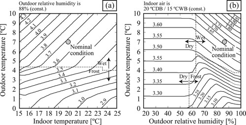
Figure 28(a) shows the COP for the combination of inlet dry bulb temperature of the indoor and outdoor units. The COP values for the nominal conditions are almost identical to the specifications listed in Table 6.

Figure 28(b) shows the COP of the outdoor unit against the combination of dry bulb temperature and relative humidity. When the outdoor air temperature decreases and frost occurs, the efficiency decreases nonlinearly. If the relative humidity is low and heat is absorbed only in the dry state coil of the condenser, the effect of relative humidity becomes negligible.

4) Total energy efficiency with heat recovery with gas engine heat pump

A GHP model was developed to calculate the effect of waste heat recovery on the efficiency. The specifications of the GHP are presented in Table 8, and only the differences from Table 6 are noted.

Table 8 Specifications of gas engine heat pump.

Conditions	JIS		Example
Heating capacity	JIS nominal load condition	x	31.5	kW
	JIS mid-load condition	x	26.5	kW
Gas consumption rate	JIS nominal condition	x	14.5	kW
	JIS mid-load condition	x	9.0	kW
Air flow rate		x	210	m^3/min

The effects of waste heat recovery, outdoor air temperature, and partial load rate on the COP ratio (R_cop [-]) are shown in Figure 29. R_cop is the value obtained by dividing COP by the nominal COP as shown in the following equation. (59) $R_{cop}=COP/CO{P}_N$(59) The relative humidity of the outdoor air was kept constant at 88% that is the same as the nominal condition. Figure 29(a) shows the case without waste heat recovery, and Figure 29(b) shows the case with waste heat recovery.

Figure 29 Effect of heat recovery, outdoor-air temperature, and heat load on COP ratio.

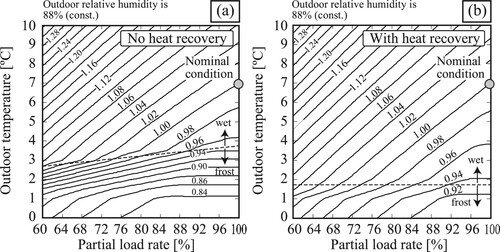
The circle plot in the figure (100%/7 °C) agrees with the performance at nominal conditions in Table 8.

When the outdoor air temperature is higher and the partial load rate is lower than the nominal condition, the R_cop value improves. This trend is almost the same in both Figure 29(a) and (b). When the outdoor air temperature drops, frost occurs and its temperature (dashed line in figures) decreases in the case of heat recovery. The decrease in R_cop is smaller when compared with the case without heat recovery. This is because with heat recovery, some part of the heat is obtained directly from the waste heat, and the effect of lower outdoor temperature is relatively small.

6. Evaluation of the model characteristics with measured data

The characteristics of the developed model were evaluated by comparing it with actual measured data.

Miyata et al. (2019) reported the results of actual measurements of a VRF system with four indoor units in the experimental chamber. The performance of the system has been measured with different combinations of the indoor unit heat load, where, few are the same as the JIS test point. Therefore, this result is convenient for the estimation of the parameters of the model developed in this study and to confirm the accuracy of the model for the extrapolation range.

The measured indoor unit heat load combinations and electricity are summarized in Tables 9 and 10. The predicted electricity of the developed model is also listed. The hatched rows (C-H1a, C-M1, H-H1, and H-M1) represent the experiments conducted in accordance with the JIS test points. The measurements in these four conditions were used to initialize the parameters of the model. The measurements in the other 19 conditions were used to evaluate the predictive performance of the model in the extrapolation range.

Table 9 Measured indoor unit heat load combinations and electricity (Cooling).

		Cooling load [kW] `					Electricity [kW]
Case		Unit 1	Unit 2	Unit 3	Unit 4	Total	Measured	Simulated
High load	C-H1a	5.49	5.89	4.72	4.73	20.83	4.43	4.42
	C-H2	1.51	5.19	4.05	4.01	14.76	2.59	2.83
	C-H3	4.70	4.88	4.41	4.03	18.02	3.37	3.58
	C-H4	4.83	4.94	2.97	3.15	15.89	2.53	2.98
	C-H5	5.13	off	4.60	4.57	14.30	2.72	2.86
Medium load	C-M1	3.08	3.19	2.93	2.95	12.15	1.90	1.91
	C-M2	3.01	3.22	3.03	2.93	12.19	1.94	1.91
	C-M3	1.06	4.07	3.44	3.27	11.84	2.01	2.05
	C-M4	1.68	1.83	3.60	3.59	10.70	1.84	1.68
	C-M5	0.78	0.96	4.45	4.53	10.72	2.01	1.90
	C-M6	4.12	off	3.53	3.61	11.26	1.95	2.18
	C-M7	5.63	5.81	off	off	11.44	2.23	2.22

Table 10 Measured indoor unit heat load combinations and electricity (Heating).

		Heating load [kW]					Electricity [kW]
Case		Unit 1	Unit 2	Unit 3	Unit 4	Total	Measured	Simulated
High load	H-H1	5.83	5.26	5.72	6.00	22.81	4.62	4.50
	H-H2	0.98	5.28	6.01	6.27	18.54	3.86	3.95
	H-H3	4.17	3.82	4.03	4.45	16.47	2.92	3.24
	H-H4	5.42	5.02	2.71	2.98	16.13	2.77	3.07
	H-H5	5.38	off	5.81	4.94	16.13	3.36	3.54
Medium load	H-M1	2.78	2.52	2.99	2.71	11.00	1.98	1.99
	H-M2	2.75	2.69	2.79	3.18	11.41	2.03	2.16
	H-M3	5.07	1.87	2.77	2.61	12.32	2.13	2.36
	H-M4	1.03	0.76	4.58	4.74	11.11	2.13	2.17
	H-M5	3.93	off	4.10	3.70	11.73	2.30	2.39
	H-M6	off	off	5.60	6.05	11.65	2.59	2.82

In the report of Miyata et al., two experiments (C-H1a and C-H1b) were conducted under nominal conditions; however, one of them resulted in an overload that exceeded the nominal capacity of the outdoor unit; therefore, the results of this experiment were not used in this study. Because the results under the mid-load and mid-temperature conditions were not reported, the performance curves were initialized from the results of the nominal condition and mid-load condition only.

A comparison between the actual measured values and the predicted values of electricity obtained via simulation is shown in Figure 30. The simulation results agree with the measured value under both the nominal and mid-load conditions as well as under the other indoor unit load combinations. For the same medium heat load, the trend of higher electricity is predictable when there is a high partial load indoor unit (C-M7 and H-M6).

Figure 30 Comparison between the actual measured values and the predicted values of electricity by simulation.

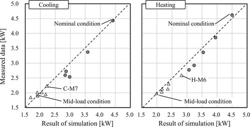
7. Sensitivity analysis coupled with building model

Combining the building heat-load calculation model with the VRF model, a case study was conducted on the impact of VRF specifications on the annual energy consumption.

7.1 Development of building and VRF model

1) Specification of target building

A room on the south side of a standard office building, as defined under Japan’s energy conservation law (the Act on Rationalizing Energy Use), was used for the case study. The floor plan and air conditioning zones are shown in Figure 31. The area of each indoor unit was zoned to be approximately 50 m².

Figure 31 Plan and air conditioning zone.

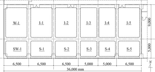
Details of the specifications of this building are given in SHASE (2016) and are therefore not provided here. Popolo (Togashi 2016), a thermal environmental simulation library, was used for the simulation, and its accuracy was reported by Ono, Ito, and Yoshida (2017), comparing the result with EnergyPlus and others.

2) Specification of VRF

The capacity of VRF system to be calculated was designed using the following procedure.

The heat load calculation model was used to estimate the annual hourly heat load of each air-conditioning zone. Using the peak cooling sensible heat load (H_spk [W/m²]) and the floor area (A_fl [m²]), the required cooling capacity, Q_evp,peak [kW], of the indoor unit was obtained using Eq. 60, where R_SL [-] is the sensible heat ratio and R_mr [-] is the margin of safety ratio, set to 0.9 and 0.1, respectively. (60) $Q_{evp,peak}=0.001\frac{H_{spk}\cdot A_{fl}}{R_{SL}}(1+R_{mr})$(60) The indoor unit cooling capacities selected based on Q_evp,peak are summarized in Table 11. The specifications of the indoor units based on the nominal cooling capacity are listed in Table 12. The total value of the nominal cooling capacity of indoor units is 75.6 kW. An outdoor unit with a capacity of 85.0 kW was selected, with the capacity corrected based on the pipe length of 0.9. The specifications of the outdoor unit are presented in Table 13.

Table 11 Indoor-unit cooling capacities.

Zone	Maximum sensible heat load, Hspk [W/m^2]	Floor area, Afl [m^2]	Maximum total heat load, Qevp,peak [kW]	Nominal cooling capacity of indoor unit, Qevp,N [kW]
W-1	97.7	58.5	8.10	9.0
I-1	92.5	58.5	7.60	8.0
I-2	92.5	58.5	7.65	8.0
I-3	93.2	45.0	5.90	7.1
I-4	93.2	45.0	5.88	7.1
I-5	97.2	58.5	8.17	9.0
SW-1	102.1	32.5	4.66	5.6
S-1	95.9	32.5	4.38	4.5
S-2	95.9	32.5	4.39	4.5
S-3	94.3	25.0	3.34	3.6
S-4	94.6	25.0	3.34	3.6
S-5	101.6	32.5	4.69	5.6

Table 12 Indoor-unit specifications.

Nominal cooling capacity, Qevp,N [kW]	3.6	4.5	5.6	7.1	8.0	9.0
Nominal heating capacity, Qcnd,N [kW]	4.0	5.0	6.3	8.0	9.0	10.0
Air flow rate [m^3/min]	12.5	14.5	15.5	22.0	23.5	30.0
Electricity [kW]	0.028	0.037	0.043	0.072	0.086	0.128

Table 13 Outdoor-unit specifications.

-	Conditions		Value
Cooling	Capacity	JIS nominal	85.0	kW
		JIS mid-load	38.3	kW
		JIS mid-load and mid-temperature	40.2	kW
	Electricity	JIS nominal	24.8	kW
		JIS mid-load	7.58	kW
		JIS mid-load and mid-temperature	6.08	kW
Heating	Capacity	JIS nominal	95.0	kW
		JIS mid-load	42.8	kW
	Electricity	JIS nominal	25.8	kW
		JIS mid-load	8.33	kW
Fan	Air flow rate		680	m^3/min
	Electricity		0.208	kW
Pipe	Nominal length		7.5	m
	Comparison length		100	m
	Correction factor		0.90	−

Based on the specifications of these indoor and outdoor units, the parameters were estimated and the model was initialized using the method developed in Sections 3 and 4.

3) Calculation of simulation speed

The calculation speed of the developed model was measured. The computer used to measure the speed was Windows 10 Pro with Intel Core i7-8565U 1.8GHz-1.99 GHz CPU; 1 year of the simulation was repeated 10 times, and they were completed in 3.16 s per year on average. The simulation was run while loading a CSV file containing previously calculated heat load data. Because the floor area of this example is approximately 500 m², an estimated simulation time of approximately 60 s is required for an office building of approximately 10,000 m². This is fast enough to be used in design practice.

7.2 Calculation result of base case

Figure 32 shows the monthly heat load, required electricity for heating, and COP. The electricity is the sum of the compressor and the fans of the indoor and outdoor units. The COP in this section is calculated by this definition of electricity.

Figure 32 Monthly heat load, electricity requirement for heating, and COP.

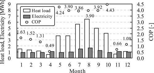
The nominal COP is 3.30 for cooling and 3.55 for heating. The COPs in the cooling season (May to October) are higher than the nominal value; however, the COP in the heating season (November to April) is much lower than the nominal value. There are two main reasons for this. The first reason being that the partial load rate of heating is extremely small and below the lower limit of capacity control. The other reason is that the compression ratio of heating is larger than that of cooling. Each of these reasons is described in detail below.

Figure 33 shows the cumulative frequency for each partial load rate. The maximum partial load rate was 61.4% for cooling and 77.2% for heating. In the case of cooling, the frequency peaks at approximately 20%, while in the case of heating, the partial load rate is less than 5% most of the time. Due to the thermal storage load in winter mornings, it has a long tail shape with a large load for an extremely short duration.

Figure 33 Cumulative frequency for each partial load rate.

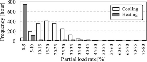
Figure 34 shows the relationship between the partial load rate and COP. In the low load range where the COP changes linearly, capacity control is not possible and the VRF system is in the on/off state. Comparing with Figure 33, it can be seen that most of the heating operation occurs in this range.

Figure 34 Relationship between the partial load rate and COP.

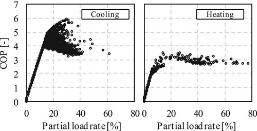
Figure 35 shows the relationship between compression ratio (R_HL) and COP. In the cooling operation, the compression ratio is small, and the COP is high. The compression ratio of the heating operation is higher than that of the cooling operation. This is because the temperature difference between indoor and outdoor is larger in winter (heating) than in summer (cooling), in Japan. The plots scattered in the lower part of the figure are the operations that are in the on/off state because they are outside the capacity control range.

Figure 35 Relationship between compression ratio (R_HL) and COP.

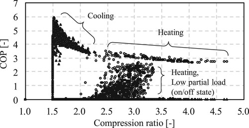
7.3 Result of sensitivity analysis

The simulation was conducted by changing few conditions from the base case. The simulation cases are shown in Table 14. Underlined items are the conditions that were changed. The simulation results for each case are shown in Table 15. Each case is detailed below.

Table 14 Simulation cases.

Case	Base	1	2	3	4-a	4-b
Maximum evaporation temperature [°C]	10	15	10	10	10	10
Minimum condensation temperature [°C]	46	41	46	46	46	46
Outdoor-unit height [m]	0	0	0	0	0	0
Pipe length [m]	100	100	7.5	100	100	100
Spray water on outdoor unit?	No	No	No	Yes	No	No
Outdoor-unit cooling capacity [%]	100	100	100	100	140	60

Table 15 Simulation results.

Case		Base	1	2	3	4-a	4-b
Cooling	Heat load [GWh/yr]	28.57	28.57	28.57	28.57	28.57	28.56
	Electricity [GWh/yr]	7.09	6.27	7.00	6.54	7.59	7.22
	COP [-]	4.03	4.56	4.08	4.37	3.76	3.96
Heating	Heat load [GWh/yr]	6.32	6.32	6.33	6.32	6.33	6.16
	Electricity [GWh/yr]	4.32	4.10	4.24	4.32	4.68	3.89
	COP [-]	1.47	1.54	1.49	1.47	1.35	1.58
Annual	Heat load [GWh/yr]	34.89	34.89	34.89	34.89	34.89	34.72
	Electricity [GWh/yr]	11.41	10.37	11.24	10.86	12.28	11.11
	COP [-]	3.06	3.36	3.10	3.21	2.84	3.13

1) Sensitivity to evaporation and condensation temperature controllable range

When the heat load of the indoor unit is small, it can cool and heat even if the temperature difference between the refrigerant and air is small. Such control reduces the compression ratio and decreases energy consumption. In Case 1, the evaporation temperature on cooling can be controlled to a maximum of 15 °C and the condensation temperature on heating to a minimum of 41 °C. The COP for both cooling and heating increased by approximately 10%.

Figure 36 shows the change in compression ratio (R_HL). Compared with the base case, the compression ratio was reduced by approximately 10%.

Figure 36 Change in compression ratio (R_HL).

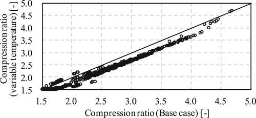
2) Sensitivity to pipe length change

The longer the refrigerant piping, the lower is the capacity caused by pressure loss in the piping. As summarized in Table 13, the capacity decreases by 10% (i.e. the correction factor is 90%) when the pipe length is increased from 7.5 m to 100 m under nominal conditions. However, as can be seen from the results of Case 2 listed in Table 15, the annual energy consumption changes only slightly (from 11.41–11.24). The pressure drop decreases rapidly as the refrigerant flow rate decreases because the pressure drop in the piping is proportional to the square of the volumetric flow rate. As shown in Figure 33, many operations had a partial load rate of less than 30%; therefore, the effect of pressure drop is considered small on a yearly basis.

3) Effect of water spray on outdoor unit

Spraying water on an outdoor unit lowers the dry bulb temperature and increases the temperature difference with the refrigerant that lowers the condensation pressure and lowers the compression ratio, thereby, improving the efficiency. Comparing the base case and case 3 presented in Table 15, the annual COP shows an improvement from 3.06–3.21.

The relationship between relative humidity and electricity ratio is shown in Figure 37. The electricity ratio is the electricity without water spray to the electricity with water spray. The lower the relative humidity, the lower is the electricity ratio because the dry bulb temperature is significantly reduced by evaporation. However, when the partial load rate is low, the compression ratio is already close to the lower limit; therefore, the effect of water spraying is minimal. The horizontal plot shown in the upper part of the figure represents the operation.

Figure 37 Relationship between outlet-air relative humidity and electricity ratio.

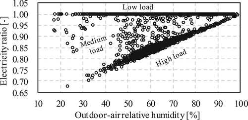
Table 16 lists the change in compressor electricity with water spraying. It can be seen that the monthly average relative humidity is almost the same; however, the electricity ratio is lower from July to September, when the average partial load is higher than that in the other months.

Table 16 Changes in compressor electricity consumption upon water spray.

	May	Jun.	Jul.	Aug.	Sep.	Oct.	Annual
Average outdoor-air relative humidity [%]	63.2	74.7	74.5	72.9	74.4	62.8	70.4
Average partial load [%]	15.4	14.6	21.7	24.7	19.1	16.8	18.7
Electricity (base case) [GWh]	0.87	0.95	1.46	1.65	1.27	0.92	7.13
Electricity (spray) [GWh]	0.84	0.90	1.32	1.48	1.15	0.89	6.58
Electricity ratio [-]	0.96	0.95	0.90	0.89	0.91	0.97	0.97

4) Sensitivity of outdoor-unit capacity

When the rotation speed can be controlled by the inverter, the efficiency increases as the heat load decreases. However, when it reaches the lower limit of the capacity control, it attains an on/off state, and the efficiency starts to decrease. To evaluate the effect of this convex characteristic of efficiency, the nominal capacity of the VRF system was varied.

Because outdoor units in the market are composed of several basic units of the different COPs, the nominal COP of each machine differs depending on the capacity. To eliminate the effect of such differences among machines and to evaluate the effect of partial load rate, the cooling/heating capacity was varied by simply increasing or decreasing the specifications proportionally listed in Table 13.

When the capacity is increased by 40%, the COP decreases for both cooling and heating because the time period in the less efficient on/off state increases (Case 4-a). The operation in the on/off state increases from 1,403 h in the base case to 1,921 h.

When the capacity is reduced by 40%, the annual COP increases; the on/off state time period decreases from 1,403 h in the base case to 815 h (Case 4-b). The COP of heating is improved, though the COP of cooling is decreased. This is because the effect of increasing the partial load and decreasing the efficiency was greater than the effect of decreasing the on/off state and increasing the efficiency. As shown in Figure 33, the distribution of the cooling partial load rate is wide; therefore, it is difficult to solve the above trade-off and select the optimal cooling capacity.

8. Discussion

The energy performance of VRF systems is affected by various factors, such as winter frost, unbalanced heat loads of indoor units, and changes in evaporation and condensation temperatures. The impact of these factors on the performance is nonlinear and difficult to express in a performance curve that is expressed as a simple polynomial. Furthermore, in a real building, few such factors may change simultaneously, making it even more difficult to predict their combined impact on energy.

Thus, this study proposes a model that uses physical models of the evaporator and condenser to calculate the refrigeration cycle. Using this model, the effects of changes in various elements can be expressed in a single index, the compression head of the refrigeration cycle. Figures 26 and 28 show that the performance characteristics of the VRF system have a complex shape with inflection points as the conditions change.

A typical office building was used as an example to evaluate the effect of VRF performance characteristics on the annual energy. The impact of several factors on the energy performance of the VRF system was measured quantitatively by using the developed model. The effect of pipe length on the capacity of a VRF system is expressed as a ‘correction factor.’ However, its effect on annual energy consumption was smaller than this factor because the refrigerant flow rate reduced at low loads, and the pressure drop had a lower effect on energy consumption. The effectiveness of the water spray depends on the combination of the partial load rate of the VRF system and the outdoor air conditions; the effect was greater from July to September when the partial load was higher.

If the capacity of the equipment was designed to be excessively large (140% to base case), the COP of both cooling and heating was decreased because the partial load rate was lowered. Further, even when the capacity was reduced, the COP of the cooling system decreased because it was out of the efficient operating point. These results indicate that the performance of VRF systems vary based on the use of the building and the design of the VRF; therefore, further case studies are required.

In this study, a method to estimate the parameters of the model from the JIS test point information is presented. The evaporation and condensation temperatures of the refrigerant have a significant effect on the estimation of the parameters of the heat exchanger. Although it was estimated based on previous studies and models in this study, it is necessary to obtain more reliable values at these temperatures to further improve the accuracy of the model. For example, in a chilled water coil, the inlet water temperature is provided as essential information that specifies the heat exchange performance of the coil. Similarly, the refrigerant state should also be considered as essential information and provided for direct expansion coils.

The model remains to be improved in some aspects.

The model is static, and the performance characteristics in the range below the capacity control are assumed, as shown in Figures 15 and 24. Furthermore, as can be seen from the distribution of partial load rate in Figure 33, the VRF system operates for a considerable amount of time at a partial load rate smaller than the lower limit of capacity control. Therefore, the energy prediction performance in this operating range has to be improved further. However, to achieve this, dynamic components of the VRF system, such as accumulators or gas–liquid separators, must be introduced to make the model dynamic. This is not an easy problem because it makes parameter estimation even more difficult, and the time required for annual simulation is longer.

In this study, no model was presented for the heat recovery ventilator with a direct expansion coil. Once the required cooling (or heating) capacity and evaporation (or condensation) temperature are calculated, the same calculation method as that for normal indoor units can be applied; therefore, modelling this will not be difficult.

The calculation in the case of overload remains to be improved. As shown in Figures 16 and 26, this model cannot provide more energy than the nominal head; therefore, it cannot provide capacity when the conditions are more severe than the nominal conditions. However, according to Miyata's (2019) actual measurements, for example, real machines can also provide cooling capacity above the nominal value. Perhaps real machines are designed with a capacity margin. To express this, it would be better to set a value larger than the nominal head as the upper limit of the iterative calculation, as shown in Figures 10 and 21. However, it is not clear how much higher than the nominal head can be set as the maximum value; therefore, it remains to be investigated further.

The heat recovery operation with simultaneous cooling and heating is considered a difficult aspect for the model improvement. Because the refrigeration cycle changes depending on whether the priority is cooling or heating (Zhang et al. 2018b), this modelling cannot be performed without investigating the underlying mechanism of the control of actual machines.

Although a sensitivity analysis was also conducted in this study, the effect of an unbalanced heat load of the indoor unit on the energy consumption should be further investigated in the future. Although the developed model has enabled energy prediction under this condition, the type of unbalanced load that should be set as a condition is not yet established. To solve this problem, models of the elements that cause unbalanced loads in actual buildings, such as, office-holder behaviour, would also have to be developed.

Acknowledgements

This work was supported by JSPS KAKENHI [Grant Number JP 18K04462].

Disclosure statement

No potential conflict of interest was reported by the author(s).

Additional information

Funding

This work was supported by Japan Society for the Promotion of Science KAKENHI [grant number JP 18K04462].

References

- Aoki, K., M. Hattori, and T. Itoh. 1985. “A Study of Extended Surface Heat Exchanger with Frosting: 1st Report, Overall Heat Transfer Characteristics.” Transactions of the Japan Society of Mechanical Engineers Series B 51 (469): 3048–3054. https://doi.org/https://doi.org/10.1299/kikaib.51.3048.
- ASHRAE (American Society of Heating, Refrigerating and Air-Conditioning Engineers, Inc.). 1997. “ASHRAE Handbook Fundamentals”.
- ASHRAE (American Society of Heating, Refrigerating and Air-Conditioning Engineers, Inc.). 2004. “ASHRAE Handbook HVAC Systems and Equipment”.
- Aynur, T. N. 2010. “Variable Refrigerant Flow Systems: A Review.” Energy and Buildings 42 (7): 1106–1112. https://doi.org/https://doi.org/10.1016/j.enbuild.2010.01.024.
- DOE (Department of Energy). 2019. “Variable Refrigerant Flow Heat Pumps.” EnergyPlus Version 9.2.0 Documentation, Engineering Reference, 1161–1220.
- Fujii, T., S. Murakami, H. Inishi, and T. Yanai. 2009. “Development of an Integrated Energy Simulation Tool for Buildings and MEP Systems, the BEST, Part51 - Characteristics of Heat Source Appliances and Packaged Air Conditioners.” Technical Papers of Annual Meeting the Society of Heating, 687–690. https://doi.org/https://doi.org/10.18948/shasetaikai.2009.2.0_687.
- Honda, Y., and K. Sano. 1999. “Latest Technology Trends of Electric Motors for Air Conditioner Compressors.” The Journal of The Institute of Electrical Engineers of Japan 119: 512–515. https://doi.org/https://doi.org/10.1541/ieejjournal.119.512.
- Hong, T., K. Sun, R. Zhang, R. Hinokuma, S. Kasahara, and Y. Yura. 2016. “Development and Validation of a New Variable Refrigerant Flow System Model in EnergyPlus.” Energy and Buildings 117: 399–411. https://doi.org/https://doi.org/10.1016/j.enbuild.2015.09.023.
- Inoue, U. 2008. “Air Conditioning Handbook,” 296, ISBN:978-4-621-07959-1 C3052.
- Ishibashi, A., and T. Matsuda. 2017. “Development of a Heat Exchanger for Air Conditioner.” International Journal of Refrigeration 92 (1080): 16–19.
- JIS Committee. 2015. “JIS B 8615-3: 2015, Multiple split-system air-conditioners and air-to air heat pumps – Testing and rating for performance”.
- JIS Committee. 2015. “JIS B 8616: 2015, Package air conditioners”.
- JIS Committee. 2015. “JIS B 8627: 2015, Gas engine driven heat pump air conditioners”.
- JSRAE (Japan Society of Refrigerating and Air Conditioning Engineers). 2006. “JSRAE Handbook, Part II Equipments”, 66–68.
- Kays, W. M., and A. L. London. 1984. “Compact Heat Exchangers,” 3rd ed. Malabar, FL: Krieger Publishing Company.
- Lian, Z., S. Park, W. Huang, Y. Baik, and Y. Yao. 2005. “Conception of Combination of Gas-Engine-Driven Heat Pump and Water-Loop Heat Pump System.” International Journal of Refrigeration 28: 810–819. https://doi.org/https://doi.org/10.1016/j.ijrefrig.2005.02.004.
- Lin, X., H. Lee, Y. Hwang, and R. Radermacher. 2015. “A Review of Recent Development in Variable Refrigerant Flow Systems.” Science and Technology for the Built Environment 21 (7): 917–933. https://doi.org/https://doi.org/10.1080/23744731.2015.1071987.
- Matsumoto, K., K. Ohno, K. Saito, and T. Kishimoto. 2015. “Evaluate VRF Compression Heat-Pump System Under Steady-State Analysis.” Transactions of the Japan Society of Refrigerating and Air Conditioning Engineers 32 (2): 95–107. https://doi.org/https://doi.org/10.11322/tjsrae.14–41.
- Miyata, M., K. Kurotori, N. Enteria, H. Yamaguchi, T. Sawachi, and Y. Kuwasawa. 2019. “Development of Energy Efficiency Estimation Method for Variable Refrigerant Flow Air-Conditioning System with Unbalanced Heat Load Operation,” Proceedings of the 16th IBPSA Conference, 1898–1905, https://doi.org/https://doi.org/10.26868/25222708.2019.210667.
- Nakagawa, Y., K. Nagawasa, S. Shiochi, K. Sato, and H. Niwa. 2011. “Research of Technology That Forecasts the Improvement Effect in Cooling Efficiency of the Multi-Air-Conditioning System by Water Spraying.” Technical Papers of Annual Meeting the SHASE, 2257–2260. https://doi.org/https://doi.org/10.18948/shasetaikai.2011.3.0_2257.
- Ono, E., S. Ito, and H. Yoshida. 2017. “Development of Test Procedure for the Evaluation of Building Energy Simulation Tools.” Proceedings of the International Building Performance Simulation Association, 380–388. https://doi.org/https://doi.org/10.26868/25222708.2019.210592.
- Ozeki, K., C. Saeki, T. Higo, and T. Kobayashi. 2001. “The Development of High Heat-Transfer Performance and Lighter Weight Inner Grooved Copper Tubes for New Refrigerant’s Applications.” Kobe Steel Engineering Reports 51 (1): 61–65.
- Saito, K., and J. Jeong. 2012. “Development of General Purpose Energy System Simulator.” Energy Procedia 14: 1595–1600. https://doi.org/https://doi.org/10.1016/j.egypro.2011.12.1138.
- Sato, K., Y. Sakamoto, S. Kametani, E. Niwa, S. Shiochi, and S. Nakano. 2008. “Development of HVAC System Simulation for Life Cycle Energy Management, Part 17: Development of Objects for Multi-Air-Conditioning System.” Technical Papers of Annual Meeting the Society of Heating, 693–696. https://doi.org/https://doi.org/10.18948/shasetaikai.2008.1.0_693.
- SHASE (Society of Heating, Air-Conditioning and Sanitary Engineers of Japan). 2010. “Handbook of air-conditioning and sanitary engineering,” 14th edition.
- SHASE (Society of Heating, Air-Conditioning and Sanitary Engineers of Japan). 2016. “SHASE-G 1008-2016, Guideline of test procedure for the evaluation of building energy simulation tool”.
- Shibata, Y. 2007. “Research and Development on Improvement in Performance of Heat Exchangers for Air-Conditioners.” The Proceedings of the Thermal Engineering Conference 2007, 25–32. https://doi.org/https://doi.org/10.1299/jsmeted.2007.25.
- Shinagawa, K., S. Murakami, H. Ishino, T. Yanai, Y. Kawazu, and T. Mori. 2018. “Study on Database Construction of Equipment Characteristics of Air Conditioning for Energy Simulation, Part 2 - Database for Central and Decentralized Cooling and Heating Equipment.” Transactions of the Society of Heating, Air-Conditioning and Sanitary Engineers of Japan 43 (253): 51–59. https://doi.org/https://doi.org/10.18948/shase.43.253_51.
- Togashi, E. 2014. “Development of Equation of State for the Thermodynamic Properties of HFC32 (R32) for the Purpose of Annual Building Energy Simulation.” Transactions of the Society of Heating, Air-Conditioning and Sanitary Engineers of Japan 39 (204): 69–76. https://doi.org/https://doi.org/10.18948/shase.39.204_69.
- Togashi, E. 2016. “The art of thermal environmental computing.” Togashi Lab. Kogakuin University, ISBN:978-4990890810.
- Torregrosa-Jaime, B., P. J. Martínez, B. González, and G. Payá-Ballester. 2019. “Modelling of a Variable Refrigerant Flow System in EnergyPlus for Building Energy Simulation in an Open Building Information Modelling Environment.” Energies 12 (1), https://doi.org/https://doi.org/10.3390/en12010022.
- William, H. P. H., S. A. Teukolsky, W. T. Vetterling, and B. P. Flannery. 2007. “Numerical Recipes 3rd Edition: The Art of Scientific Computing,” ISBN:978-0521880688.
- Yamaguchi, H., H. Niwa, M. Miura, and D. Narumi. 2005. “Study on the Improvement Effect in Cooling Efficiency of the Air Source Heat Pump Chiller by Water Spraying.” Technical Papers of Annual Meeting the SHASE, 1745–1748. https://doi.org/https://doi.org/10.18948/shasetaikai.2005.3.0_1745.
- Yamaguchi, H., H. Niwa, M. Miura, D. Narumi, and K. Nakazawa. 2006. “Study on the Improvement Effect in Cooling Efficiency of the Air Source Heat Pump Chiller by Water Spraying, Report 2: Analysis of Influence That Difference of Method and Water Volume Give to Efficiency of Water Spraying.” Technical Papers of Annual Meeting the SHASE, 1725–1728. https://doi.org/https://doi.org/10.18948/shasetaikai.2006.3.0_1725.
- Yun, G. Y., J. H. Lee, and H. J. Kim. 2016. “Development and Application of the Load Responsive Control of the Evaporating Temperature in a VRF System for Cooling Energy Savings.” Energy and Buildings 116: 638–645. https://doi.org/http://doi.org/10.1016/j.enbuild.2016.02.012.
- Zhang, G., X. Li, W. Shi, B. Wang, Z. Li, and Y. Cao. 2018a. “Simulations of the Energy Performance of Variable Refrigerant Flow System in Representative Operation Modes for Residential Buildings in the Hot Summer and Cold Winter Region in China.” Energy and Buildings 174 (1): 414–427. https://doi.org/https://doi.org/10.1016/j.enbuild.2018.06.064.
- Zhang, R., K. Sun, T. Hong, Y. Yura, and R. Hinokuma. 2018b. “A Novel Variable Refrigerant Flow (VRF) Heat Recovery System Model: Development and Validation.” Energy and Buildings 168: 399–412. https://doi.org/https://doi.org/10.1016/j.enbuild.2018.03.028.
- Zhang, G., H. Xiao, P. Zhang, B. Wang, X. Li, W. Shi, and Y. Cao. 2019. “Review on Recent Developments of Variable Refrigerant Flow Systems Since 2015.” Energy and Buildings 198: 444–466. https://doi.org/https://doi.org/10.1016/j.enbuild.2019.06.032.
- Zhou, Y., P. Wu, J. Y, R. Wang, Z. Shiochi, S. and Li, and Y. M. 2008. “Simulation and Experimental Validation of the Variable-Refrigerant-Volume (VRV) Air-Conditioning System in EnergyPlus.” Energy and Buildings 40 (6): 1041–1047. https://doi.org/https://doi.org/10.1016/j.enbuild.2007.04.025.