A data schema for exchanging information between urban building energy models and urban microclimate models in coupled simulations

Abstract

Understanding and quantifying the interactions between urban microclimate and urban buildings is essential to improve the urban environment and building performance, especially during heatwaves. Most previous studies used tool or application specific data exchange mechanisms that cannot be generalized for other tools or applications. In this paper, we introduce a new flexible and tool-agnostic data schema to facilitate the exchange of data between urban building energy models and urban microclimate models. The JSON schema was tested using a district of 97 buildings in San Francisco and running simulations with CityBES and CityFFD as the urban building energy and microclimate modeling platforms, respectively. Compared with simulation results using the historical weather data, simulation results considering interactions between two models over a two-day heatwave event showed a 5.3°C higher average peak building facade temperature, an 8.9 °C higher average peak air node temperature, and a 19.5% higher peak cooling energy use.

KEYWORDS:

• Urban building energy modeling
• Urban microclimate
• Coupled simulation
• CityFFD
• CityBES
• data model

Introduction

Mitigation of global climate change impacts calls for decarbonization of building stocks to reduce energy use and greenhouse gas (GHG) emissions, as well as improvements of buildings and urban environment to be resilient against increasing risks due to the more frequent, intense, and longer duration extreme weather events such as heatwaves, cold snaps, and wildfires. The United Nations’ Sustainable Development Goal 11 (SDG 11) emphasizes the inclusive, safe, resilient, and sustainable performance of cities under such extreme weather conditions (Al-Zu’bi and Radovic 2018). In an urban environment, adjacent buildings influence each other, and buildings interact with the urban microclimate. Understanding and quantifying the interactions between urban microclimate and urban buildings is essential to improve the urban environment, e.g. predicting and reducing the urban heat island (UHI) effect (Adilkhanova, Ngarambe, and Yun 2022) and building performance for energy efficiency, demand flexibility, and climate resilience (Reinhart and Davila 2016), (Hong et al. 2020). Urban microclimate (local conditions of ambient air temperature, humidity, wind speed and direction, solar irradiance) influences urban building performance, including a building’s energy use, peak demand, indoor environmental quality, and heat emissions from the building to ambient air. Meanwhile, urban buildings influence the urban microclimate through heat emissions, the release of air pollutants, and the wind shielding effect (Kikegawa et al. 2003; Kikegawa et al. 2006; Ihara et al. 2008). Such two-way interactions need to be quantified and understood under normal weather conditions and, more importantly, during extreme weather events such as heatwaves, cold snaps, and wildfires. Methods to quantify these interactions need to consider various spatial resolutions (from a building surface to a whole building to a district of buildings) and temporal resolutions (from sub-seconds to minutes to hours).

Urban Building Energy Modeling (UBEM, Hong et al. 2020) usually refers to the bottom-up physics-based approach to modeling each individual building in a district of buildings or a city’s entire building stock while considering influences between buildings (e.g. shading) and between buildings and the urban microclimate (Hong et al. 2021). Integrating the urban microclimate effects in UBEM yields a more accurate assessment of building energy consumption in urban areas (Vallati et al. 2015). From the perspective of UBEM, the urban microclimate data could be obtained from three sources (Hong et al. 2020): (1) observational weather data, (2) a data-driven forecasting model, and (3) a physics-based forecasting model. The most traditional approach is to obtain weather data (e.g. ambient air temperature, humidity, pressure, wind speed, and solar radiation) from either measurements at remote open areas (e.g. airports near large cities) or historical datasets, which are usually compiled as a typical meteorological year (TMY) weather file for the past 30 years (Liu et al. 2017), (Hong, Chang, and Lin 2013). However, these measured weather data usually fail to capture the actual microclimate effects in urban areas, especially for specific blocks and districts (Mylona 2012). Measuring the high-resolution weather data around the targeted urban buildings may mitigate the limitation of this approach. For instance, websites such as Weather Underground and Dark Sky, as well as other weather application programming interfaces (APIs) such as Cal-Adapt and Open Weather Map, provide a wealth of data from different local weather stations. These resources enable users to access hyper-local, historical, or near real-time weather observations for their specific UBEM cases.

Recently, a data-driven weather forecasting approach became popular to provide more accurate and real-time weather data for UBEM, which benefited from the mass production of affordable and user-friendly weather stations, as well as the increasing technology of automated measurements and data model analysis. Tools such as Urban Weather Generator (Bueno et al. 2013) and Weather Shift (Troup and Fannon 2016) morph rural weather data and historical high-frequency weather data, respectively, to forecast the future urban weather data given different future-period emission scenarios (e.g. Representative Concentration Pathway [RCP] scenarios). This approach generates flexible weather data for specific UBEM cases, consuming less computational resources compared with physics-based weather forecasting approaches. However, its limitations lie in its coarse resolution and ignoring the two-way interactions between buildings and the urban environment, which can be significant when assessing the building energy use in urban areas.

Driven by the increased necessity of higher resolution and detailed boundary information, as well as the recent advances in computing infrastructure, the third approach, physics-based weather forecasting, remains popular for simulating and predicting the urban microclimate. Two examples of this are generating urban canopy models by computational fluid dynamics (CFD) and fast fluid dynamics (FFD). Particularly, co-simulation between UBEM and an urban microclimate model (UCM) is necessary to capture the two-way interactions between buildings and the surrounding urban environment.

Urban weather boundary conditions such as ambient air temperature, humidity, pressure, wind speed and direction, solar irradiation, and specular and diffuse reflections can greatly influence UBEM results. Similarly, buildings also influence the urban microclimate boundary conditions as (1) thermal interactions between building envelope (exterior surfaces or building skin) and urban environment through heat transfer and mass flow, and (2) heat and moisture release from buildings through cooling towers, condensing units, and exhaust air to the urban environment. Studies in the past decade have presented different methods to conduct coupling of building energy models (BEMs) and urban microclimate models. Yang et al. (Yang et al. 2012) developed a framework coupling the UCM model ENVI-met and BEM model EnergyPlus to exchange urban boundary conditions using the Building Controls Virtual Testbed (BCVTB) co-simulation platform. CitySim (Vermeulen, Kämpf, and Beckers 2013) introduced a coupling architecture based on the embedded UCM solver to exchange environmental variables with the EnergyPlus model in real time, applying the functional mockup interface (FMI) co-simulation standard. The SOLENE microclimate model (Gros et al. 2016) was presented to model microclimate and building thermal interactions, considering the combined thermal effects among the atmosphere, building surfaces, and indoor air. Katal et al. (Katal, Mortezazadeh, and Wang 2019) developed the coupled model between CityFFD (City Fast Fluid Dynamics) and CityBEM (City Building Energy Model) to perform co-simulations at the city scale.

Jain et al. (Jain et al. 2020) presented a novel one-way coupling methodology incorporating a weather research and forecasting (WRF) model and EnergyPlus, with a goal of evaluating the impact of urban weather boundary conditions on the energy performance of urban buildings. Vahmani et al. (Vahmani et al. 2022) developed a process-based WRF-UCM-EnergyPlus coupling framework to enhance the current understanding of feedback processes between anthropogenic heating from buildings and urban microclimate dynamics. Luo et al. (Luo et al. 2020) coupled a high-resolution urban microclimate model, URF-UCM, with prototype EnergyPlus building energy models to quantify the anthropogenic heat emissions from buildings and interactive effects of urban microclimate and building heat emission in terms of the urban energy balance. The UCM-WRF-CityFFD coupling strategy was proposed for evaluating the airflow and thermal conditions inside urban street canyons with different aspect ratios and different anthropogenic temperature increments under heatwaves (Mortezazadeh, Jandaghian, and Wang 2021). An integrated multi-scale and multi-physical urban microclimate model based on WRF-UCM-OpenFOAM-EnergyPlus was used for the urban thermal environment and urban heat island (UHI) mitigation study, accounting for the impacts of mesoscale weather conditions and building energy performance in the urban microclimate analysis (Wong et al. 2021). The urban microclimate model ENVI-met was integrated with the transient 3D BES software TRNSYS (Transient System Simulation) to accurately model and simulate the influence of urban form and vegetation on city microclimates (Perini et al. 2017), as well as the space heating/cooling energy demand of buildings with the impact of urban microclimate (Dorer et al. 2013). Detommaso, Costanzo, and Nocera 2021 integrated ENVI-met and UWG (Urban Weather Generator) to overcome the lack of on-site measured urban meteorological data in the calibration of urban microclimate modeling. A novel holistic workflow of Honeybee-Ladybug-Dragonfly was introduced to simulate the thermal interaction of buildings with outdoor space at the district scale in a Grasshopper environment (Evola et al. 2020). López-Cabeza et al. 2022 developed and further validated a methodology for the simulation of courtyards in buildings by integrating BES and CFD simulations using the Ladybug Tools.

These coupling frameworks and tools show different potentials to produce high-resolution simulation results of building thermal behaviours interacting with the local microclimate. The difficulty of these co-simulation setups lies in that UCMs and UBEMs are usually developed to run simulations at very different spatial and temporal resolutions. First, UBEM usually runs simulations for each individual building (dimensions ranging from 1 to 100 meters) that considers each building exterior surface, such as exterior walls, roofs, and windows, while UCM runs simulation at a computational domain of several kilometers or even tens of kilometers. Second, UBEM usually runs at 10, 15, or 60 min time steps, while urban microclimate CFD models run at a few second to a few minute time steps, depending on the size of the computational domain, grid resolutions near building objects, inlet wind speed, and numerical models of turbulence solvers. Choosing a suitable time step depends on the stability of the CFD model.

Most of the aforementioned studies used co-simulation frameworks, such as FMI, for data exchange in run time between models. This enables the exchange of simulation variables with EnergyPlus or other BEMs at each time step. However, these run-time data exchange frameworks mostly use tool-or-application-specific data exchange mechanisms that cannot be generalized or adopted for other tools or applications. The variables to exchange, and the spatial and temporal resolutions to conduct the data exchange, are designed case by case. Because of the different resolutions of the UBEM and UCM models, different co-simulation mechanisms are required when coupling building surface boundary conditions to urban canopy cells. Hence, a standard data exchange schema is needed to provide a more convenient path to design such co-simulation frameworks, regardless of the simulation and coupling resolutions used by different simulation models or tools.

In this study, we developed a novel, flexible, and tool-agnostic semantic schema (in JSON) to facilitate the exchange of data between UBEM and UCM. The schema can be used across scales (city block, district, or entire city or region) and for various UBEM and UCM tools. The JSON schema was tested using a district of 97 buildings in San Francisco, California, USA, and running simulations with CityBES as the UBEM tool and CityFFD as the UCM tool. This paper contributes to developing and demonstrating a flexible and tool-agnostic JSON schema to facilitate the data exchange between the urban building energy models and the urban microclimate model during the co-simulation. The JSON schema can be used across scales (from a district with 100 buildings to an entire city with 100k buildings). In this paper, although the schema was demonstrated by the case study using two specific tools, it can be adopted by other UBEM and urban CFD tools.

Method

Microclimate modeling and simulation with CityFFD

CityFFD is a UCM tool based on semi-Lagrangian and fractional step methods with a group of novel numerical schemes to improve the model’s accuracy and reduce its computational cost (Mortezazadeh and Wang 2017; Mortezazadeh and Wang 2019; Mortezazadeh and Wang 2020). CityFFD has been equipped with a fourth-order numerical interpolation scheme that reduces numerical dissipation and dispersion errors even on coarse grids (Mortezazadeh and Wang 2017). This model was written based on graphics processing units (GPUs) with the CUDA-C++ programming (GPU-CUDA) and OpenMP to access GPUs for large-scale parallel computing. It was recently shown that CityFFD could model large-scale problems quickly on personal computers (Mortezazadeh, Jandaghian, and Wang 2021), (Mortezazadeh and Wang 2020). CityFFD captures the turbulence behaviour of the airflow in the atmospheric boundary layer by using Large Eddy Simulation (LES) (Mortezazadeh and Wang 2020). Currently, CityFFD can read non-uniform structured mesh. Using the semi-Lagrangian approach, CityFFD is an unconditionally stable model for different mesh sizes or time steps: for example, a range of grid resolutions from 1 meter (m) to 10 m near the buildings can be applied depending on the computational domain size and available hardware.

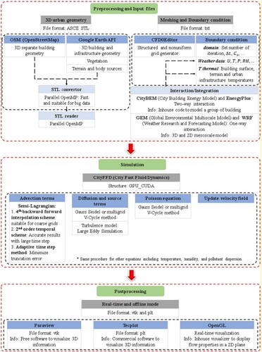
CityFFD has three main steps to model urban microclimate, as shown in Figure 1:

1. Preprocessing: This part of the model is based on OpenMP. In this section, the geometry of the domain, which includes building geometry and terrain, will be uploaded to the platform (Mortezazadeh et al. 2022) in the ASCII STL (stereolithography) format. Other building geometry information, such as different surfaces, location of the surfaces, roofs, etc., will be recognized. Depending on the UBEM model, this information will be provided by a text or JSON file. Other input data, including weather data and mesh information, are uploaded into the simulation engine at this stage.

2. Simulation: The numerical model for solving conservation equations has been written based on GPU-CUDA. Data and variables will be transferred into the graphic card memory. Then the simulation is conducted on the graphics card. At the end of the simulation, the data are transferred back for the post-processing step.

3. Post-processing: At this step, different outputs are generated. One output is generating air velocity vectors and contours and representing microclimate data inside the domain. This output format can be vtk or plt, and different tools can be used to visualize the data, such as Paraview (Ahrens, Geveci, and Law 2005) or Tecplot (MITCHELL 2000). The second output is the local microclimate data near the buildings. The data are used as inputs to UBEM tools. For example, here, the JSON data are generated at the end of each simulation for CityBES to provide wind speed, direction, and temperature near each surface of each building.

Figure 1. Workflow of CityFFD (adopted from Mortezazadeh et al. 2022).

Building energy and heat emission simulation with EnergyPlus

EnergyPlus is the U.S. Department of Energy’s flagship building energy software for simulating building energy and environmental performance. In addition to considering buildings’ thermal loads, the system response to those loads, and the resulting energy use, EnergyPlus also employs a bottom-up approach to simulate and report the run-time calculated building heat emissions at the thermal zone and building levels (Hong et al. 2020). In EnergyPlus, heat emissions are calculated, aggregating heat generated from the envelope, zones, and heating, ventilation, and air conditioning (HVAC) systems. The reported building heat emissions come from (1) convective and radiative heat emissions from the envelope to the ambient air, (2) exhaust and relief heat through air exfiltration of the building envelope and the HVAC system relief moist air, and (3) sensible and latent heat rejection through HVAC systems such as condensing units (e.g. direct expansion [DX] coils, cooling towers) and combustion equipment (e.g. fuel boilers, gas furnaces).

In this study, the hourly total heat emission rates for each surface and the entire building in watts are calculated and reported during the simulation period. For each exterior surface of a building, the total heat is calculated as the convective and radiative heat emission rate from the surface, added with the HVAC exhausted and rejected heat emission rate at the zone and building level subdivided to all exterior surfaces proportionally by surface area. The heat flux feeding into any CityFFD grid cell is then calculated as the total heat amount of the attached surfaces divided by the connected area with the CityFFD grid cell.

UBEM with CityBES

CityBES (i.e. City Buildings, Energy, and Sustainability, formerly City Building Energy Saver) (Hong et al. 2016) is one of the UBEM programs (Ferrando et al. 2020). CityBES is a web-based data and computing platform that focuses on energy modeling and analysis of a city’s building stock to support district- or city-scale energy efficiency programs (Hong et al. 2016). CityBES uses an international open data standard, CityGML, to represent and exchange 3D city models. CityBES employs EnergyPlus to simulate building energy use and savings from energy-efficient retrofits (Chen, Hong, and Piette 2017). CityBES provides a suite of features for urban planners, city energy managers, building owners, utilities, energy consultants, and researchers.

Figure 2. Workflow of CityBES.

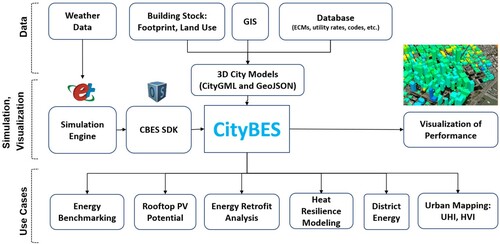
CityBES has a three-layer architecture (Figure 2): the Data layer, the Algorithms and Software layer, and the Use Cases layer. The Data layer includes the weather data; the 3D city model (CityGML or GeoJSON) created with multiple data sources such as GIS, land use, and assessor records (Chen et al. 2019); and a database of energy efficiency measures, utility rates, and building energy codes and standards. The Software layer includes EnergyPlus as the simulation engine and CBES SDK, which is a software development kit built upon OpenStudio to create EnergyPlus models. The Use Cases layer provides examples of applications, including energy benchmarking, energy retrofit analysis, district heating, and cooling system modeling (Li et al. n.d), renewable energy analysis, building performance visualization, and heat resilience modeling (Sun et al. 2021), as well as urban scale mapping of microclimate (Hong et al. 2021) and heat vulnerability at the census tract level (Xu et al. 2021).

The building dataset used by CityBES (Chen et al. 2019) can be either in GeoJSON or CityGML format. In addition to the building geometry, it requires several essential building characteristics for simulation, such as year of build, number of stories, and building type. The information is usually consolidated from land use data, LiDAR data, tax assessor data, real estate APIs, and other local open data sources. When being simulated, some of the building geometries may be simplified at the back end of CityBES. For the purposes of data exchange, the actual geometries used in the simulation process will be shared with CityFFD to ensure both tools use the same geometry as the boundary conditions.

Data and coupling mechanisms

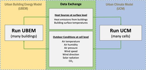
Figure 3 illustrates the general data exchange fields and process to couple UBEM and UCM models. At each iteration, the UBEM provides heat emission and building surface temperature per exterior surface at the boundary conditions for the UCM, while UCM provides local ambient conditions for the UBEM at the CFD cell level, which may include ambient air temperature, humidity, pressure, wind speed and wind direction, solar radiation, and carbon dioxide (CO₂) level.

Figure 3. Data exchange between UBEM and UCM.

Previous studies conducted coupling simulations using tool- or application-specific data exchange mechanisms that cannot be generalized and adopted for other tools or applications. This work develops a new flexible and tool-agnostic JSON schema to facilitate the exchange of data between the UBEM and UCM tools. Figure 4 shows the sketch of the proposed data exchange schema. Five JSON files were designed to facilitate the entire data exchange process, considering different types of information to exchange (static versus dynamic). First, based on the geographic information, UCM and UBEM tools each generate a JSON file containing the static geographic information (i.e. centroids of the building surfaces and the CFD grid cells) for all UCM grid cells, as well as UBEM buildings and surfaces, respectively, as shown in file No. 1 and file No. 2 in Figure 4. Specifically, for the UCM tool, the name of each grid cell was identified as continuous ID, and the centroid of each grid cell was clearly defined based on geographic information. Similarly, for the UBEM tool, the names of each building and its surfaces were identified as continuous ID as well, while the centroids of each building and each surface were defined based on the same geographic information as the UCM tool. Then, a JSON file (file No. 5 in Figure 4) was created to map UBEM buildings and their surfaces to UCM grid cells based on the static information provided in file No. 1 and file No. 2.

Figure 4. Illustration of the data exchange schema using five JSON files.

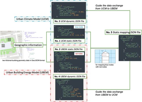
These three static JSON files build up the ‘bridge’ to transfer the simulated data between both sides. Every grid cell ID in the UCM tool was mapped with one or multiple surface IDs in the UBEM tool. Later, in each coupling iteration, the UCM tool outputs the simulated variables for each grid cell ID, including the air dry bulb temperature, wind speed, and wind direction, as shown in file No. 3 in Figure 4. These UCM data were transferred to particular buildings and their surfaces based on the mapping IDs in file No. 5. Similarly, the simulated UBEM data for each surface or building, such as the temperature, heat emission, and other related variables, were transferred to the corresponding UCM grid cell based on the mapping IDs as identified in file No. 5.

Since the data in file No. 3 and file No. 4 were updated between each iteration, these two files were dynamically changed during the co-simulation, while the three static JSON files—file No. 1, file No. 2, and file No. 5—were directly coming from the geographic information of the simulation domain.

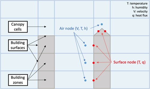
Figure 5 further illustrates the mechanism of mapping building surface and ambient air condition data via air nodes (UCM/CityFFD domain) and surface nodes (UBEM/CityBES domain). Surface nodes (red nodes) represent the UBEM building exterior surfaces, including exterior walls, roofs, and windows. Air nodes (blue nodes) represent the UCM cells that hold surrounding air conditions. The nearest red nodes and blue nodes were mapped based on the centroid information. Generally speaking, during the later coupled simulations, a red node reads outdoor conditions from its mapped blue node, and a blue node takes the aggregated heat flux and individual surface temperature from its attached/mapped surfaces as boundary conditions.

Figure 5. Mechanism of mapping the grid cells in UCM (blue nodes) with the building surfaces in UBEM (red nodes).

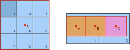
In practice, depending on the different resolutions of the building surface and CFD grid size, there were occasions that one red node mapped to multiple blue nodes (CFD cells) (Figure 6 (a)) and occasions that one blue node mapped to multiple red nodes (building surfaces) (Figure 6 (b)). For the former scenario, each blue grid (grids 1–9) took the total heat emission flux from Surface A, and the heat transfer flux from the surface to each cell was calculated as the total emission divided by the total ‘attached’ area of the nine grids. For the surface temperature, a uniform and constant temperature of the red node was set for all grids in the CFD model. In the meantime, Surface A reads the air properties from the nearest grid to the centroid of the surface, which is Grid 5. For the latter scenario, the blue grids pre-scanned their ‘attached’ surfaces, and the total heat of all the attached surfaces was added to the corresponding cell. For example, in Figure 6 (b), Surface A and Surface B are attached to Grid 1, and the total heat and area-weighted temperature of the two surfaces are fed to Grid 1, while Surface C is attached to Grid 2 and serves as the boundary condition for Grid 2. One surface can only be attached to one grid, so the heat would not be double-counted. Each of the three surfaces in Figure 6 (b) takes local air conditions from the nearest grid to its centroid, similar to the first scenario.

Figure 6. (a). One surface node (red) mapping to multiple air nodes (blue); (b): One air node (blue) mapping to multiple surface nodes (red).

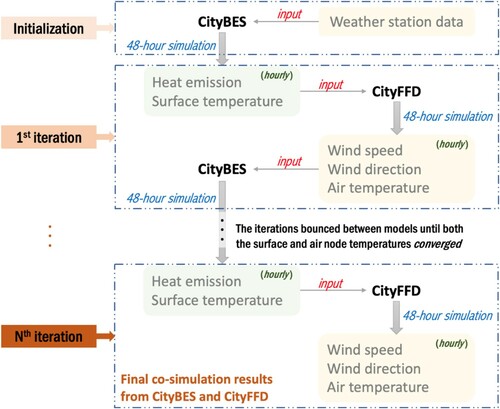
The co-simulation workflow is illustrated in Figure 7. We took the entire 48-hour simulation period as one iteration and ran simulations from each side of the coupling: the CityBES building energy models and the CityFFD urban microclimate model. Generally, these two tools run at different spatial and temporal resolutions, with the proposed JSON schema facilitating the data exchange. Specifically, after the initial CityBES simulation using the historical weather station data, the hourly surface node data (i.e. heat emission and surface temperature) in JSON format was fed to kick off the first iteration of the CityFFD simulation. Accordingly, the hourly air node data (i.e. wind speed, wind direction, and air temperature) in JSON format was then fed back to CityBES as the updated weather files. The iterations bounced between the CityBES and CityFFD models until both the surface and air node temperatures converged. The converging criteria in this study were set when the hourly average of all exterior surface temperatures in the simulation domain between rounds of iterations was below 0.3°C (Tsoka, Tsikaloudaki, and Theodosiou 2018).

Figure 7. Workflow of the co-simulation between CityBES and CityFFD.

Results

The data exchange schema

According to the data exchange mechanism, as shown in Figure 4, we created five JSON files to clearly describe the geometry relationship, data fields, and resolution to be used for the initialization of both models and the run-time exchange.

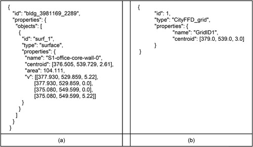
Figure 8 (a) and (b) present the JSON files to store and describe the static geographic information of both the red and blue nodes for the initialization of both UBEM and UCM models and the mapping of the data exchange nodes. Figure 8 (a) and (b) are the file No. 2 and file No. 1 in Figure 4. The red node JSON stores the vertex coordinates, centroid coordinates, area, and ID for each building surface, and the blue node JSON stores the centroid coordinates and ID for each air node.

Figure 8. Static information description for (a) a surface node and (b) an air node, in JSON format.

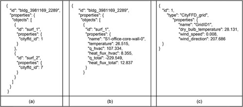
According to the static geometry information, a static mapping JSON file (Figure 9 (a)) was created by pre-scanning and assigning the mapping information between the red and blue nodes to be used in run-time data exchange (Figure 9 (b)). For example, the surface surf_1 of the building bldg_3981169_2289 was mapped to the grid/cell of cityffd_id 1. Finally, Figures 9 (b) and (c) present the run-time data exchange files between models written at each time step. In this study, the simulation time steps for CityBES and CityFFD were ten minutes and five seconds, respectively. While the data exchange between CityBES and CityFFD was done at the hourly time step, when a surface node fed an air node with its temperature (°C), equivalent HVAC and total heat emission weighted to a certain surface (W), and heat fluxes normalized by the surface area (W/m²); an air node then fed a surface with its temperature (°C), wind speed (m/s), and wind direction (degree).

Figure 9. (a) Static mapping information for the simulation; (b) the run time data exchange file from surface nodes to air nodes; (c) the run-time data exchange file from air nodes (blue) to surface nodes (red).

The case study

A neighbourhood of 97 buildings in northeast San Francisco was selected as the case study (Figure 10) to test the data exchange schema. All the building information was collected from the public data portal of San Francisco, DataSF [datasf.org]. The dataset comprises 78 office buildings and 19 retail buildings of various sizes.

Figure 10. CityBES dataset of 97 buildings for the San Francisco case study. The weather station and the sample 20-floor office building are highlighted.

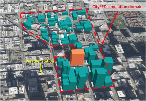
We conducted the case study for a recent heat wave event in San Francisco, California, USA. Historically, the city observes a mild climate (climate zone 3C), with a warm and dry summer. However, in recent years, unprecedented heat waves have hit the city more frequently during the summer season. On September 1, 2017, the city set an all-time heat record in the downtown area at 41.1°C (106°F), and the heat wave lasted three days. We performed a 48-hour simulation for the two hottest days—September 1 and 2, 2017—initializing the CityBES and CityFFD models with the 2017 historical weather data collected from the local weather station in downtown San Francisco.

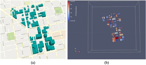
The EnergyPlus models were created using CityBES for each of the 97 buildings with multiple zoning on each floor and run at a ten-minute time step; while the CityFFD microclimate model was created for the domain (900 meters by 900, and 350 meters in height) with a grid size of two meters in three dimensions, and run at a five-second time step. The CityBES model and the CityFFD model are shown in Figure 11 (a) and (b), respectively. The total grid number of the CityFFD domain is about 35 million. The ground temperature was set to 40°C based on a recent research that derived land surface temperature images from Landsat 8 satellite thermal infrared sensor from 2017 to 2020 in the San Francisco Bay area (Potter and Alexander 2021). The data exchange between CityBES and CityFFD occurred at the hourly time step, which is considered one timestep of the co-simulation. The CityFFD was running on a 64-core 256 MB RAM computer with one NVIDIA Tesla V100 GPU card, consuming about 50 min for each coupling time step. The CityBES was running on the same machine, consuming less than 10 min for each coupling time step.

Figure 11. Simulation model in (a) CityBES and (b) CityFFD.

EnergyPlus, the simulation engine used in CityBES, calculates the building heat emission by five components - zone exfiltration, zone exhaust air, HVAC system heat rejection, HVAC system relief air, and building exterior surface convection heat. The zone exfiltration and exhaust heat and the surface convective heat were averagely associated with the building envelope surfaces, while the HVAC system heat rejection (counted as the total heat, not split into sensible and latent parts) from the cooling tower was associated with the roof surfaces where the cooling tower was located. During the co-simulation, we aggregated the associated waste heat for each surface (red node), and then passed the data to its surrounding air node (blue node) in CityFFD as the boundary conditions.

Within the simulation district, there are 33 buildings (accounting for 6.7% of the total building floor area of the selected neighbourhood) excluded from the CityBES simulations due to the lack of building information. Those buildings are mostly residential. Although their waste heat is ignored, their shading effects on the surrounding buildings are considered in the simulations.

Figure 12 shows the hourly average exterior surface temperature of a sample 20-floor office building in the 97-building district. The blue line represents the hourly average temperature of all exterior surfaces of the building for the initialization round using the weather station data. The figure shows that after three rounds (r1 to r3) of iterations, the surface temperatures converged. The peak temperature at the converged round reached 55.5°C at 2 pm on September 2, while the peak temperature at the initialization round was 50.2°C at the same hour.

Figure 12. Average exterior surface temperatures of a sample office building.

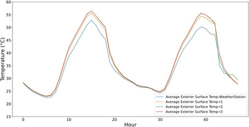
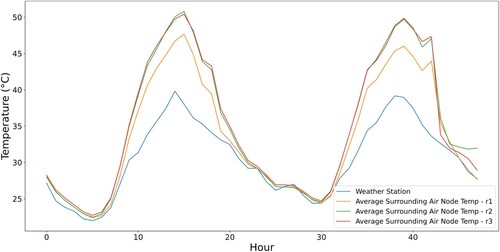
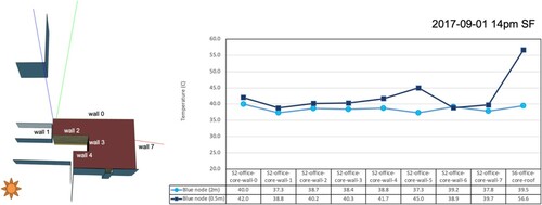
Figure 13 shows the hourly average air node temperatures surrounding the sample building. The calculation of the airflow in the boundary layer (e.g. the 1st and 2nd grid near-ground) will be less accurate than those in the outer layers, because the current version of CityFFD does not have wall functions for both velocity and temperature. For large urban scale simulations, the Y + values are typically large so a wall function can improve the accuracy. On the other hand, our previous validation study at the urban scale showed acceptable accuracy for the outer layers and regions away from the surface without the wall functions (Mortezazadeh et al. 2022). So in this study, we chose the third grid from the wall to reduce the possible impacts of interpolations near the wall. This is a limitation of CityFFD itself and we plan to implement wall functions to improve the simulation of near surfaces whereas this will not affect the proposed data schema. Similar to the results of the building exterior surface temepratures, the air temperatures also converged after three rounds of iterations. The average and peak temperatures of the historical weather station were 30.4°C and 40.6°C during the two-day period, while the average and peak temperatures of the surrounding air nodes were 35.1°C and 49.7°C, about 20% higher than the peak temperature from the historical weather data.

Figure 13. Average air temperature of local air nodes of a sample office building.

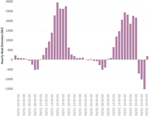
We also calculated the hourly total heat emissions from the sample high-rise office building to the ambient air across 48 h from September 1 to September 2, as shown in Figure 14. The building absorbed heat from the surrounding air during the early morning until 9 am, and then started to produce heat emissions to the ambient air for the rest of the day. The peak hourly heat emission reached 3,000 megajoules (MJ) and 2,500 MJ on the first and second day of the heat wave period, respectively, both at about 4–6 pm. The heat emissions from the building quickly decreased to almost zero or even negative after 8 pm in the evening. The total daily heat emissions from the sample building to the ambient air were 16.7 gigajoules (GJ) and 12.1 GJ on September 1st and September 2nd, respectively. The daily heat emission on the first day (Sep 1st, Friday) was 38% higher than that on the second day (Sep 2nd, Saturday), which was due to the office building having higher HVAC loads and heat exhaust during the weekday than the weekend.

Figure 14. Hourly heat emission of a sample office building.

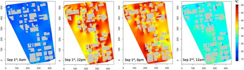
The heat emissions from buildings during the daytime largely affect the ambient temperature near buildings, thus the surrounding atmosphere in the entire domain. Figure 15 shows the temperature distribution of outdoor air nodes within the simulation domain in the sixth, twelfth, eighteenth, and twenty-fourth hours of September 1. As aforementioned, all air nodes were chosen as the third grids from the ground (an elevation of 5 m) to avoid the boundary effect or any numerical errors in the near-ground areas. In the early morning, the air temperature near buildings was about 20°C, and there was no heat emission from the nearby buildings, as shown in Figure 14. At noon, the air temperature near the buildings increased to almost 50°C, while the ambient air temperature was about 38°C. As indicated in Figure 14, the buildings began to produce heat emissions to the surrounding air starting at 10 am, which accelerated the heating of the surrounding air afterward. The heat emissions from buildings reached the highest temperature at about 5 pm, when the air temperature near the buildings was higher than 50°C, while the ambient air temperature reached 42°C in most places. The peak temperature of the historical weather station (as highlighted in Figure 10) was 40.6°C during the two-day period, and that occurred at 3 pm on September 1. By comparison, the average temperature of the simulated air nodes was higher than the historical record, due to the higher temperature of the near-building air nodes which were heated by building surfaces. However, the simulated temperature of those air nodes in the open space matches the historical record well (with a difference of 0.4°C). Until midnight, the air near buildings was gradually cooled to less than 20°C, while the ambient air temperature was still about 25°C.

Figure 15. Ambient air temperature distribution of the entire simulation domain (at an elevation of 5 m) at morning, noon, afternoon, and midnight on September 1.

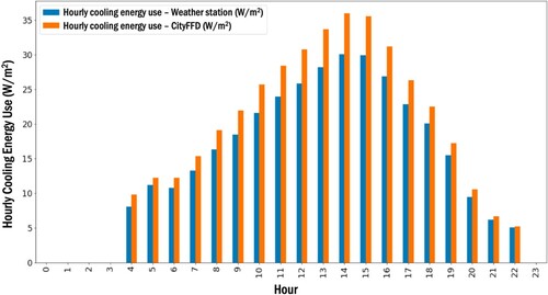
We also compared the total building cooling energy use intensity (EUI) between the weather station (first iteration) round, and the final converged round on the second day of the simulation (a normal working day with a regular office cooling schedule). Figure 16 plots the cooling energy use averaging across all 97 buildings in the simulation domain. The average and peak hourly cooling energy use from the CityBES simulations for the weather station round were 14.3 and 30.1 W/m², while the average and peak hourly cooling energy use with the coupled simulations between CityBES and CityFFD were 16.7 and 36.0 W/m², 16.5% and 19.5% higher than the results from the weather station round. In reality, the buildings generate a lot of waste heat to the surrounding air increasing their temperature; in return, the increased air temperature affects the building operations by increasing the cooling loads, which leads to more cooling energy use and associated heat emissions. The traditional building energy modeling - taking the historical weather data from an existing weather station as the boundary input – does not capture the local context considering heat exchange interactions between the buildings and the surrounding urban environment. The co-simulation in this work captures this two-way interaction, which yields a more accurate calculation of the building cooling energy use.

Figure 16. Comparison of the simulated hourly building cooling energy use with the static historical weather data and the dynamic simulated microclimate data.

Discussion

We propose a data schema using a set of five JSON files to facilitate and standardize the data exchange between two simulation domains in UBEM and UCM. Particularly, the mapping JSON file (the No. 5 file in Figure 4) generated based on the static geographic information was designed to ensure the two computing domains are consistent for further data exchange. Theoretically, one surface of one building in UBEM will be mapped with one grid in UCM to avoid any unbalanced data exchange in the next step. However, in practice, depending on the resolutions of building surface and CFD grid size in different UBEM and UCM tools, there are occasions when one building surface can be mapped to multiple CFD grids and occasions when one CFD grid can be mapped to multiple building surfaces. While the building surfaces sample a small subset of surrounding air nodes to capture local ambient air conditions, the air nodes read the aggregated heat flux from all building exterior surfaces to ensure the total building and domain level heat transfer from buildings are included in the CityFFD microclimate modeling. The concept of ‘attached’ surfaces was designed to ensure there are no miscounted or double-counted heat fluxes. Therefore, the simulated heat fluxes are correctly transferred between two simulation domains. Depending on the grid resolution in CityFFD and reading the building surfaces, it is possible that some surfaces are replaced with some other surfaces. So, to capture the information of each of these missed surfaces, we must find the particular surface that replaces them. This surface is then named as an ‘attached’ surface.

Traditional two-way co-simulation usually performs ping-pong coupling at each simulation time step, which requires a reset of simulation status at the beginning of each time step and multiple iterations to converge at each time step. In this study, we tested a coupled simulation technique by expanding the ping-pong time horizon for the convergence to the whole 48-hour simulation period and checked convergence using predetermined criteria. The tested coupled simulation technique aims to reduce the number of iterations and, thus, the computing time for both the UBEM and UCM models while ensuring certain simulation accuracy. Current results indicate that three iterations are adequate to find a converged solution when the hourly average of all exterior surface temperatures in the simulation domain between two adjacent rounds of iterations are below 0.3°C (Tsoka, Tsikaloudaki, and Theodosiou 2018). We believe this is one of the first studies proposing and demonstrating this new coupling strategy for urban-scale simulations. Further studies need to verify whether the time horizon, the CFD grid resolution or the size of domains (e.g. number of buildings and number of CFD grid cells) will influence the number of iterations required for the coupled simulation to converge, as well as whether there is a more reasonable converging criterion.

In most cases, the distance between two building surfaces is larger than 2 m, which is the grid resolution in this case study. However, for some specific buildings (e.g. concave buildings), there might be scenarios when the distance of two surfaces is less than the grid resolution, which may induce inaccuracy in the simulation. We compared the simulated surface temperature under the grid resolution of 2 and 0.5 m, respectively, with an example of two buildings in downtown San Francisco. As shown in Figure 17, the temperature difference is normally less than 2°C, except for the building roof surface.

Figure 17. Comparison of the surface temperature under the grid resolution of 2 and 0.5 m in CityFFD.

It should be noted that the simulation results shown in Figures 14–16 were not validated due to the lack of measurements. This is a limitation of the study.

In an ongoing study, we are further testing the proposed data schema and extending the simulation domain to the entire city of San Francisco, which covers an area of 121 km² and contains about 150,000 buildings. The simulated data from two tools will be exchanged at a much larger scale, which emphasizes the significance of the data schema proposed in this work. The exploration of the urban-scale building energy consumption under the extreme heat wave condition could inform the evidence-based design and lead towards achieving SDG 11 in the near future.

Conclusions

We developed an extensible and tool-agnostic data schema in JSON format to facilitate the exchange of data between urban building energy models and urban microclimate models to capture their two-way interactions. A set of five JSON files were used to facilitate the entire data exchange process by first generating the two static JSON files containing the geographic information for each building surface and each CFD grid, then mapping the building surfaces with CFD grids, and finally transferring the required data between each pairing-nodes of UBEM and UCM tools. A new coupled simulation technique was tested using CityBES as the urban building energy modeling platform and CityFFD as the urban microclimate modeling platform for a district of 97 buildings in San Francisco, during an unprecedented heat wave in September 2017. In this case, three iterations were adequate to find a converged solution when the hourly average of all exterior surface temperatures in the simulation domain between rounds of iterations were below 0.3°C. Results indicate that compared to building energy simulation with the historical local weather data, the coupled simulation, considering simulated microclimate weather conditions and heat exchange between the buildings and the surrounding urban environment, showed a 5.3°C higher peak building facade average temperature, an 8.9 °C higher peak air nodes average temperature and a 19.5% higher peak cooling energy use during the two heatwave day simulation period. The total daily heat emissions from the envelope surfaces of the sample building to the ambient air were 0.97 MJ/m² and 0.70 MJ/m² during the first and second day of the heat wave, respectively.

Acronyms

API	=	Application Programming Interface
BCVTB	=	Building Controls Virtual Testbed
BEMS	=	Building Energy Models
CFD	=	Computational Fluid Dynamics
CityBES	=	City Buildings, Energy, and Sustainability
CityFFD	=	City Fast Fluid Dynamics
DX	=	Direct Expansion
EUI	=	Energy Use Intensity
FFD	=	Fast Fluid Dynamics
FMI	=	Functional Mock-up Interface
GHG	=	Greenhouse Gas
GPU	=	Graphics Processing Unit
HVAC	=	Heating, Ventilation, and Air Conditioning
LIDAR	=	Light Detection and Ranging
RCP	=	Representative Concentration Pathway
TMY	=	Typical Meteorological Year
TRNSYS	=	Transient System Simulation
UBEM	=	Urban Building Energy Model
UCM	=	Urban Microclimate Model
UHI	=	Urban Heat Island
UWG	=	Urban Weather Generator
WRF	=	Weather Research Forecasting

Acknowledgements

The LBNL team’s work was supported by the Laboratory Directed Research and Development (LDRD) Program of Lawrence Berkeley National Laboratory, provided by the Director, Office of Science, of the U.S. Department of Energy under Contract No. DE-AC02-05CH11231. Concordia team’s work was supported by the Natural Sciences and Engineering Research Council (NSERC) of Canada through the Discovery Grants Program [#RGPIN-2018-06734] and the Advancing Climate Change Science in Canada Program [#ACCPJ 535986-18].

Disclosure statement

No potential conflict of interest was reported by the author(s).

Additional information

Funding

This work was supported by Natural Sciences and Engineering Research Council of Canada: [Grant Number RGPIN-2018-06734]; Advancing Climate Change Science in Canada Program: [Grant Number ACCPJ 535986-18]; U.S. Department of Energy: [Grant Number DE-AC02-05CH11231].

References

- “https://datasf.org.”
- Adilkhanova, I., J. Ngarambe, and G. Y. Yun. 2022. “Recent Advances in Black Box and White-Box Models for Urban Heat Island Prediction: Implications of Fusing the Two Methods.” Renewable and Sustainable Energy Reviews 165: 112520. doi:10.1016/j.rser.2022.112520
- Ahrens, J., B. Geveci, and C. Law. 2005. “Paraview: An End-User Tool for Large Data Visualization.” The Visualization Handbook 717 (8).
- Al-Zu’bi, M., and V. Radovic. 2018. SDG11-Sustainable Cities and Communities: Towards Inclusive, Safe, and Resilient Settlements. Emerald Group Publishing.
- Bueno, B., L. Norford, J. Hidalgo, and G. Pigeon. 2013. “The Urban Weather Generator.” Journal of Building Performance Simulation 6 (4): 269–281. doi:10.1080/19401493.2012.718797
- Chen, Y., T. Hong, X. Luo, and B. Hooper. 2019. “Development of City Buildings Dataset for Urban Building Energy Modeling.” Energy and Buildings 183: 252–265. doi:10.1016/j.enbuild.2018.11.008
- Chen, Y., T. Hong, and M. A. Piette. 2017. “Automatic Generation and Simulation of Urban Building Energy Models Based on City Datasets for City-Scale Building Retrofit Analysis.” Applied Energy 205: 323–335. doi:10.1016/j.apenergy.2017.07.128
- Detommaso, M., V. Costanzo, and F. Nocera. 2021. “Application of Weather Data Morphing for Calibration of Urban ENVI-Met Microclimate Models. Results and Critical Issues.” Urban Climate 38: 100895. doi:10.1016/j.uclim.2021.100895
- Dorer, V., et al. 2013. “Modelling The Urban Microclimate and Its Impact on the Energy Demand of Buildings and Building Clusters.” 13th Conference of International Building Performance Simulation Association, Chamb{é}ry, France, August 26-28, 3483–3489.
- Evola, G., V. Costanzo, C. Magrì, G. Margani, L. Marletta, and E. Naboni. 2020. “A Novel Comprehensive Workflow for Modelling Outdoor Thermal Comfort and Energy Demand in Urban Canyons: Results and Critical Issues.” Energy and Buildings 216: 109946. doi:10.1016/j.enbuild.2020.109946
- Ferrando, M., F. Causone, T. Hong, and Y. Chen. 2020. “Urban Building Energy Modeling (UBEM) Tools: A State-of-the-Art Review of Bottom-up Physics-Based Approaches.” Sustainable Cities and Society, 102408. doi:10.1016/j.scs.2020.102408
- Gros, A., E. Bozonnet, C. Inard, and M. Musy. 2016. “Simulation Tools to Assess Microclimate and Building Energy - A Case Study on the Design of A New District.” Energy and Buildings 114: 112–122. doi:10.1016/j.enbuild.2015.06.032
- Hong, T., W.-K. Chang, and H.-W. Lin. 2013. “A Fresh Look at Weather Impact on Peak Electricity Demand and Energy use of Buildings Using 30-Year Actual Weather Data.” Applied Energy 111: 333–350. doi:10.1016/j.apenergy.2013.05.019
- Hong, T., Y. Chen, S. H. Lee, and M. A. Piette. 2016. “CityBES: A Web-Based Platform to Support City-Scale Building Energy Efficiency.” Urban Computing.
- Hong, T., Y. Chen, X. Luo, N. Luo, and S. H. Lee. 2020. “Ten Questions on Urban Building Energy Modeling.” Building and Environment 168: 106508. doi:10.1016/j.buildenv.2019.106508
- Hong, T., Y. Chen, M. A. Piette, and X. Luo. 2016. “Modeling City Building Stock for Large-Scale Energy Efficiency Improvements Using CityBES.” ACEEE Summer Study Conference.
- Hong, T., M. Ferrando, X. Luo, and F. Causone. 2020. “Modeling and Analysis of Heat Emissions from Buildings to Ambient Air.” Applied Energy 277: 115566. doi:10.1016/j.apenergy.2020.115566
- Hong, T., Y. Xu, K. Sun, W. Zhang, X. Luo, and B. Hooper. 2021. “Urban Microclimate and its Impact on Building Performance: A Case Study of San Francisco.” Urban Climate 38: 100871. doi:10.1016/j.uclim.2021.100871
- Ihara, T., Y. Kikegawa, K. Asahi, Y. Genchi, and H. Kondo. 2008. “Changes in Year-Round Air Temperature and Annual Energy Consumption in Office Building Areas by Urban Heat-Island Countermeasures and Energy-Saving Measures.” Applied Energy 85 (1): 12–25. doi:10.1016/j.apenergy.2007.06.012
- Jain, R., X. Luo, G. Sever, T. Hong, and C. Catlett. 2020. “Representation and Evolution of Urban Weather Boundary Conditions in Downtown Chicago.” Journal of Building Performance Simulation 13 (2): 182–194. doi:10.1080/19401493.2018.1534275
- Katal, A., M. Mortezazadeh, and L. L. Wang. 2019. “Modeling Building Resilience Against Extreme Weather by Integrated CityFFD and CityBEM Simulations.” Applied Energy 250: 1402–1417. doi:10.1016/j.apenergy.2019.04.192
- Kikegawa, Y., Y. Genchi, H. Kondo, and K. Hanaki. 2006. “Impacts of City-Block-Scale Countermeasures Against Urban Heat-Island Phenomena Upon A Building’s Energy-Consumption for Air-Conditioning.” Applied Energy 83 (6): 649–668. doi:10.1016/j.apenergy.2005.06.001
- Kikegawa, Y., Y. Genchi, H. Yoshikado, and H. Kondo. 2003. “Development of A Numerical Simulation System Toward Comprehensive Assessments of Urban Warming Countermeasures Including Their Impacts upon the Urban Buildings’ Energy-Demands.” Applied Energy 76 (4): 449–466. doi:10.1016/S0306-2619(03)00009-6
- Li, H., T. Hong, and Z. Wang. 2021. Modelling and Simulation of District Heating and Cooling Systems Using CityBES. IBPSA Building Simulation Conference.
- Liu, Y., R. Stouffs, A. Tablada, N. H. Wong, and J. Zhang. 2017. “Comparing Micro-Scale Weather Data to Building Energy Consumption in Singapore.” Energy and Buildings 152: 776–791. doi:10.1016/j.enbuild.2016.11.019
- López-Cabeza, V. P., E. Diz-Mellado, C. Rivera-Gómez, C. Galán-Marín, and H. W. Samuelson. 2022. “Thermal Comfort Modelling and Empirical Validation of Predicted Air Temperature in Hot-Summer Mediterranean Courtyards.” Journal of Building Performance Simulation 15 (1): 39–61. doi:10.1080/19401493.2021.2001571
- Luo, X., P. Vahmani, T. Hong, and A. Jones. 2020. “City-Scale Building Anthropogenic Heating During Heat Waves.” Atmosphere 11 (11): 1206. doi:10.3390/atmos11111206
- MITCHELL, K. E. 2000. “Tecplot 8.0.” Science 290 (5499): 2097. doi:10.1126/science.290.5499.2097b
- Mortezazadeh, M., Z. Jandaghian, and L. L. Wang. 2021. “Integrating CityFFD and WRF for Modeling Urban Microclimate Under Heatwaves.” Sustainable Cities and Society 66: 102670. doi:10.1016/j.scs.2020.102670
- Mortezazadeh, M., and L. L. Wang. 2017. “A High-Order Backward Forward Sweep Interpolating Algorithm for Semi-Lagrangian Method.” International Journal for Numerical Methods in Fluids 84 (10): 584–597. doi:10.1002/fld.4362
- Mortezazadeh, M., and L. Wang. 2019. “An Adaptive Time-Stepping Semi-Lagrangian Method for Incompressible Flows.” Numerical Heat Transfer, Part B: Fundamentals 75 (1): 1–18. doi:10.1080/10407790.2019.1591860
- Mortezazadeh, M., and L. L. Wang. 2020. “Solving City and Building Microclimates by Fast Fluid Dynamics with Large Timesteps and Coarse Meshes.” Building and Environment 179: 106955. doi:10.1016/j.buildenv.2020.106955
- Mortezazadeh, M., L. L. Wang, M. Albettar, and S. Yang. 2022. “CityFFD – City Fast Fluid Dynamics for Urban Microclimate Simulations on Graphics Processing Units.” Urban Climate 41: 101063. doi:10.1016/j.uclim.2021.101063
- Mylona, A. 2012. “The use of UKCP09 to Produce Weather Files for Building Simulation.” Building Services Engineering Research and Technology 33 (1): 51–62. doi:10.1177/0143624411428951
- Perini, K., A. Chokhachian, S. Dong, and T. Auer. 2017. “Modeling and Simulating Urban Outdoor Comfort: Coupling ENVI-Met and TRNSYS by Grasshopper.” Energy and Buildings 152: 373–384. doi:10.1016/j.enbuild.2017.07.061
- Potter, C., and O. Alexander. 2021. “Impacts of the San Francisco Bay Area Shelter-in-Place During the COVID-19 Pandemic on Urban Heat Fluxes.” Urban Climate 37: 100828. doi:10.1016/j.uclim.2021.100828
- Reinhart, C. F., and C. C. Davila. 2016. “Urban Building Energy Modeling – A Review of a Nascent Field.” Building and Environment 97: 196–202. doi:10.1016/j.buildenv.2015.12.001
- Sun, K., W. Zhang, Z. Zeng, R. Levinson, M. Wei, and T. Hong. 2021. “Passive Cooling Designs to Improve Heat Resilience of Homes in Underserved and Vulnerable Communities.” Energy and Buildings 252: 111383. doi:10.1016/j.enbuild.2021.111383
- Troup, L., and D. Fannon. 2016. “Morphing Climate Data to Simulate Building Energy Consumption.” Proceedings of SimBuild.
- Tsoka, S., A. Tsikaloudaki, and T. Theodosiou. 2018. “Analyzing the ENVI-met Microclimate Model’s Performance and Assessing Cool Materials and Urban Vegetation Applications–A Review.” Sustainable Cities and Society 43: 55–76. doi:10.1016/j.scs.2018.08.009
- Vahmani, P., X. Luo, A. Jones, and T. Hong. 2022. “Anthropogenic Heating of the Urban Environment: An Investigation of Feedback Dynamics Between Urban Micro-Climate and Decomposed Anthropogenic Heating from Buildings.” Building and Environment 213: 108841. doi:10.1016/j.buildenv.2022.108841
- Vallati, A., A. D. L. Vollaro, I. Golasi, E. Barchiesi, and C. Caranese. 2015. “On the Impact of Urban Micro Climate on the Energy Consumption of Buildings.” Energy Procedia 82: 506–511. doi:10.1016/j.egypro.2015.11.862
- Vermeulen, T., J. H. Kämpf, and B. Beckers. 2013. “Urban Form Optimization for the Energy Performance of Buildings Using CitySim.” in CISBAT.
- Wong, N. H., et al. 2021. “An Integrated Multiscale Urban Microclimate Model for the Urban Thermal Environment.” Urban Climate 35: 100730. doi:10.1016/j.uclim.2020.100730
- Xu, Y., T. Hong, W. Zhang, Z. Zeng, and M. Wei. 2021. “Heat Vulnerability Index Development and Mapping.” SimAUD Symposium.
- Yang, X., L. Zhao, M. Bruse, and Q. Meng. 2012. “An Integrated Simulation Method for Building Energy Performance Assessment in Urban Environments.” Energy and Buildings 54: 243–251. doi:10.1016/j.enbuild.2012.07.042