Coupled mass and heat transfer modelling in building envelopes to consistently assess human exposure and energy performance in indoor environments

Abstract

We develop a numerical model coupling heat and chemical transfers in the building envelope to predict human exposure to pollutants and heating load as affected by changes in temperature and building design. We characterize the effect of temperature variation by season and location on chemical emission dynamics from building materials and the resulting human exposure. Peak concentrations of organics are sensitive to temperatures, and increasing indoor temperature by 10°C doubles the maximum indoor air concentration reached by both VOCs and SVOCs contained in a vinyl flooring. SVOCs mean concentration over the flooring lifetime increases by a factor of 2, and, as a result, the fraction of chemical taken in by the occupants increases by 50%. Occupants’ exposure to SVOCs emission in the city of Lille is likely to increase by 20% in 2050 because of temperature increase induced by climate change.

Keywords:

• heating load
• mass balance
• chemical diffusion
• intake fraction
• building envelope
• organic chemicals

1. Introduction

The construction sector has been recognized as a major hotspot of energy use and substantial efforts have been made to promote energy-efficient buildings. Design and renovation standards tend to increase building envelope airtightness, while materials and paintings being used represent new sources of pollutants. Newly constructed buildings in which particular attention has been paid to increase air tightness are confined spaces in which a wide variety of organic chemicals are released from building materials and expose occupants to multiple health hazards (Beko et al. 2013). Worldwide, indoor pollution has been raised as a significant public health issue, since we spend on average more than 85% of our time in closed spaces (Klepeis et al. 2001). If the impact of early design choices on buildings’ thermal behaviour is now well apprehended, substantial efforts must be made to guide designers towards a good indoor air quality (IAQ). Learning how to design healthy energy-efficient buildings is one of tomorrow’s challenges.

Many studies have experimentally shown temperature dependence of the emission rate (Haghighat and De Bellis 1998; De Bellis, Haghighat, and Zhang 1995; Liang and Xu 2014; Myers 1985) and indoor air concentration of chemicals in building materials (Gaspar et al. 2014; Macintosh et al. 2012; Pilka et al. 2014). Indeed, the release of chemicals from solid materials and their sorption depends on both diffusion and partition coefficients that are specific for a chemical-material combination and temperature-dependent (Huang et al. 2017b; Huang and Jolliet 2018). The convective mass transfer coefficient, which drives the exchange between the boundary layer air immediately adjacent to the surface of the material and the bulk indoor air, is also dependent on temperature (Wei, Mandin, and Ramalho 2018).

Indoor temperature is influenced by the exchanges with the outdoor. Consequently, indoor temperature has daily and seasonal variations according to the outdoor temperature, the solar radiation, the internal heat gain and the building materials and insulation. In the Western European environmental context, indoor temperatures range from 19°C on average during winter up to 26°C during summer. Indoor temperature during summer is not controlled for the majority of European household (for example, the French Environment and Energy Agency reported that a quarter of French households are equipped with air conditioning). In this case, the temperature at materials’ inner surface can experience 10°C variation throughout the day (Hunt and Gidman 1982). With an HVAC system, the difference of temperature between the outermost material of the building envelope in contact with outdoors with the innermost material at the setpoint temperature can be in the order of 10 degrees.

To faithfully transpose real environmental conditions, the impact of temperature on the aforementioned parameters needs to be integrated when modelling emission and indoor fate of organics contained in building materials. In addition, heat and mass transfers should be treated jointly in order to ensure consistent evaluation of building design choices’ influence on both human exposure and heating load. Indeed, some design solutions, such as ventilation, for example, will impact indoor air quality directly (dilution of pollutants) and indirectly (effect on indoor temperature when it is not constrained by heating or cooling). In the same way, the choice of the material (e.g. insulation) influences, as a function of its thermal (e.g. conductivity), the heating load to reach the setpoint (heating consumption). Besides, since the temperature within the material envelope influences substance diffusion and emission, the choice of the material directly influences the substance concentration in the gaseous phase (indoor air quality) as a function of its physico-chemical properties (e.g. enthalpy of vapourization), as well as by its ability to conduct heat or not.

To better guide building design, modelling tools are needed to assess both energy demand and air quality in a common framework. Note that in this study, we focus on volatile organic compounds (VOCs) according to the definition of NF ISO 16000-6: (2012) (boiling point between 100°C and 260°C), and semi-volatile organic compounds (SVOCs) with a boiling point between 260°C and 400°C. Manifold models for dynamic heat transfer have been developed over the past 50 years (see Harish and Kumar 2016) for a review, but only several models have been developed to tackle this issue. For example, CONTAM (Dols and Polidoro 2015) and COMIS (Feustel 1998) are aeraulic models able to treat the transfers of particles or gaseous substances in the environments and in the ventilation networks. Both can be coupled with dynamic thermal simulation tools; however, none of them models pollutants emission from the building envelop. The COwZ model (Stewart and Ren 2006) models emissions to air from different types of sources including materials and adsorption/desorption phenomena by materials, but does not integrate temperature variations within the building envelope. Yan et al. (2009) proposed a tool to predict the indoor distribution of air temperature and VOCs concentration in a simultaneous way but not in a coupled way: their model does not account for the dependence of VOCs’ emission and transport mechanisms on temperature. Wei, Ramalho, and Mandin (2019) developed a dynamic model predicting SVOCs concentration indoors, which accounts for the effect of different environmental factors on SVOCs’ emission, including observed temperature. However, temperature is an input data at each time step of the model. Therefore, this model requires prior monitoring of temperature at building surfaces and in the room air that is not suitable for the building design phase.

In this paper, we aim to address the interaction between chemical mass and heat transfers in order to evaluate how early building design choices affect both human indoor exposure and energy demand. More specifically, we address the following specific objectives: (a) to develop a numerical model coupling heat and chemical transfers in the building envelope, (b) to analyse the mass balance, emission rate and indoor exposure of VOCs and SVOCs embedded in materials at standard temperature, (c) to characterize the effect of temperature and its variation by season and location on the dynamics of chemical emissions from building materials, indoor fate and human exposure, and (d) to analyse the impact of selected design solutions on heating load and human exposure to indoor emissions.

To meet these objectives, we first set up a numerical model coupling heat and mass transfers in buildings. Then, the emission and mass balance of three organics contained in a vinyl flooring are studied at standard temperature and further compared under real conditions. Finally, the impact of air renewal rate on both heating load and intake fraction of indoor chemical emissions is quantified.

2. Material and methods

2.1. Modelling heat and mass conservation

The effect of relative humidity on chemicals emission has not reached a consensus within the scientific community. Clausen et al. (2007) showed that the emission rate of DEHP was independent of the relative humidity in indoor air. Besides, Wei, Mandin, and Ramalho (2018) concluded that it remains unknown whether emissions of semi-volatile organic compounds are affected by the humidity in the source material and Huang et al. (2017b) didn’t include the relative humidity in their quantitative structure–property relationship for estimating Kma since its influence is unclear. Therefore, it has not been included in this study.

On the contrary, many studies have experimentally shown the temperature dependence of building materials’ emission rate (Haghighat and De Bellis 1998; De Bellis, Haghighat, and Zhang 1995; Liang and Xu 2014; Myers 1985) and indoor air concentration (Macintosh et al. 2012; Pilka et al. 2014; Gaspar et al. 2014). The mass transfer model used in this study accounts for the temperature evolution in the building envelope that is calculated thanks to the sensible heat transfer model.

Since the focus of this study is the evolution of the temperature in the building envelope, the thermal balance has been simplified by considering only the sensible heat. The thermal contributions by latent heat have not been considered, thus we neglected moisture transport (by vapour convection or diffusion when the water is in its gaseous state, and by capillary transport when the water is in its liquid state).

In real buildings, it is common to have multi-layer materials (e.g. a floor can consist of three layers, a vinyl flooring, a concrete layer and a waterproofing sheet). Thus, to simulate chemical emissions from and heat transfers in building materials in a real-world setting, building envelope is modelled as six functional elements (one ceiling, one floor and four sidewalls), each functional element being composed of several materials. Each material can be a source to the indoor environment and a sink for emission from other elements.

To reduce the complexity of the model, the following assumptions are made for both energy and mass conservation modelling:

1. heat and mass transfers are considered as a one-dimensional phenomenon

2. each layer of material is homogeneous

3. the building system is in contact with only one zone (i.e. outdoor compartment) represented by a single node

4. the gas medium (i.e. indoor air) is considered as well-mixed dry air

Considering assumption (Haghighat and De Bellis 1998) (only one outdoor node) and since we primarily focus on the indoor environment, we do not consider longwave radiative exchange of the outdoor surfaces with the sky and the ground separately. Table 1 details mass and heat transfer mechanisms considered in the model at the different nodes of the system.

Table 1. Analogy between heat (left column) and mass (right column) transfer mechanisms considered in the model at different system nodes.

	Heat transfer	Mass transfer
Nodes i within a material layer	Conduction following Fourier law (1a) ${\rho }_i{c}_{p_i}{S}_{i}d{L}_i\frac{d{T}_i}{dt}=\frac{2{\lambda }_i{S}_i}{d{L}_i+d{L}_{i-1}}(T_{i-1}-T_i)-\frac{2{\lambda }_i{S}_i}{d{L}_i+d{L}_{i+1}}(T_i-T_{i+1})$(1a)	Diffusion following Fick’s law (1b) $S_{i}d{L}_i\frac{d{C}_i}{dt}=\frac{2D_{m_i}(T)S_i}{d{L}_i+d{L}_{i-1}}(C_{i-1}-C_i)-\frac{2D_{m_i}(T)S_i}{d{L}_i+d{L}_{i+1}}(C_i-C_{i+1})$(1b)
Nodes i at the interface between two materials	Heat transfer at materials interface (2a) ${\rho }_i{c}_{p_i}{S}_{i}d{L}_i\frac{d{T}_i}{dt}=\frac{2{\lambda }_i{S}_i}{d{L}_i+d{L}_{i-1}}(T_{i-1}-T_i)-\frac{2S_i}{\frac{d{L}_i}{{\lambda }_i}+\frac{d{L}_{i+1}}{{\lambda }_{i+1}}}(T_i-T_{i+1})$(2a)	Mass transfer at materials interface (2b) $\begin{array}{r}{S}_{i}d{L}_i\frac{d{C}_i}{dt}=\frac{2D_{m_i}(T)S_i}{d{L}_i+d{L}_{i-1}}(C_{i-1}-C_i)-\frac{2S_i}{\frac{d{L}_i}{D_{m,i}(T)}+\frac{K_{ma,i}(T)}{K_{ma,i-1}(T)}\frac{d{L}_{i-1}}{D_{m,i-1}(T)}}\left(C_i-\frac{K_{ma,i}(T)}{K_{ma,i-1}(T)}{C}_{i-1}\right)\end{array}$(2b)
Nodes si at material inner surface	(3a) $\begin{array}{l}{\rho }_{si}{c}_{p_{si}}{S}_{si}d{L}_{si}\frac{d{T}_{si}}{dt}=h_{v,si}(T)S_{si}(T_{in}-T_{si})-\frac{2{\lambda }_{si}{S}_{si}}{d{L}_{si}}(T_{si}-T_{si-1})+h_{r_{si}}(T)S_{si}\\ \sum _{SI=1}^6{F}_{si-SI}(T_{SI}-T_{si})+(1-{\alpha }_{fl}){\alpha }_{si}{F}_{fl\to si}\sum _w^{N_w}{F}_w{S}_w{E}_{GLO}\end{array}$(3a)	(3b) $\begin{array}{l}{S}_{j}d{L}_j\frac{d{C}_{s{i}_j}}{dt}=-S_j{h}_{m,j}(T)\left(\frac{C_{si,j}}{{K_{ma}}_j(T)}-C_{in}\right)+\frac{2D_{m_j}(T)S_j}{d{L}_j}(C_{1_j}-C_{s{i}_j})\\ -\frac{f_{\text{dust}}}{K_{md}(T){\rho }_{\text{dust}}}(N_{\text{pers}}ingR)-\frac{K_{p,aq}(T)}{K_{mw}(T)}\text{FQ}{\text{S}}_{\text{ski}{\text{n}}_{\text{contact}}}\end{array}$(3b)
Indoor air node in	(4a) ${\rho }_{in}{c}_{in}V\frac{d{T}_{in}}{dt}=-\sum _{si=1}^6{h}_{v,si}(T)S_{si}(T_{in}-T_{si})-Q{\rho }_{in}{c}_p(T_{in}-T_{out})+P_{heating}$(4a)	(4b) $\begin{array}{l}{V}_{\text{building}}\frac{d{C}_{\text{in}}}{dt}=\sum _{i=1}^6{S}_i{h}_{m,i}(T)\left(\frac{C_{si,i}}{K_{m{a}_i}(T)}-\frac{C_{\text{in}}}{1+K_{pa}(T)C_{TSP}}\right)-Q(C_{\text{in}}-C_{\text{out}})-N_{\text{pers}}\\ inhR{C}_{\text{in}}-N_{\text{pers}}{S}_{\text{ski}{\text{n}}_{\text{gas}}}{K}_{p,\text{gas}}(T)\frac{C_{\text{in}}}{1+K_{pa}(T)C_{\text{TSP}}}\end{array}$(4b)

With h_m (m s⁻¹) the convective mass transfer coefficient, h_v (W m⁻² K⁻¹) the convective heat transfer coefficient, h_r (W m⁻² K⁻¹) the radiative heat transfer coefficient, Q (m³ s⁻¹) the air flow rate, S (m²) the surface, dL (m) the thickness, ρ (kg m⁻³) the density, V (m³) the volume, T (K) the temperature, C (kg m⁻³) the concentration, D_m (m² s⁻¹) the diffusion coefficient, K_ma (–) the partition coefficient, N_pers (#pers) the number of persons, inhR (m³ s⁻¹ pers⁻¹) the inhalation rate, P_heating (W) the heating power, λ (W m⁻¹ K⁻¹) the conductive coefficient, c_p (J kg⁻¹ K⁻¹) the specific heat capacity at constant pressure, f_dust (–) the fraction of ingested dust that is from the considered material, F (–) the form factor, E_GLO (W m⁻²) the solar gain on vertical surfaces, α (–) the emissivity, FQ (s⁻¹) the frequency of dermal contact with the floor, S_skin,contact (m²) skin surface in contact with the floor, S_skin,gas (m²) skin gaseous uptake surface. The subscript in stands for indoor air, i for an inner node, si for inner surface, out for outdoor, pa for particle-air, ma for material-air, md for material-dust, p,aq for skin permeation coefficient via aqueous solution, p,gas gaseous-skin permeation, w for window, fl for floor, TSP for total suspended particles.

Mass transfer: The chemical transfer model proposed in this paper is based on the state-space model developed by Yan et al. (2009) and further adjusted by Guo (2013). It builds on the most widely accepted framework for modelling VOCs and SVOCs emissions from building materials, based on the diffusion of organic chemicals inside building materials, as first presented by Little, Hodgson, and Gadgil (1994), and by Little et al. (2012).

To account for the temperature dependency of chemical releases, both diffusion $D_m$ (m² s⁻¹) and partition $K_{ma}$ (–) coefficients should be estimated as a function of temperature. We therefore chose to use the quantitative property-property relationship and quantitative structure–property relationship developed by Huang et al. (2017b) and Huang and Jolliet (2018) to estimate diffusion and material-air partition coefficients, respectively. This model predicts $D_m$ and $K_{ma}$ in more than 19 different materials as a function of material type, molecular weight, octanol-air partition coefficient, enthalpy of vapourization and temperature, as defined in the USEtox database (Fantke et al. 2017). Both coefficients are calculated in each layer of the material at each time step as a function of the temperature at the respective node (Equations 1b and 2b).

The convective mass transfer coefficient $h_m$ (m s⁻¹) driving the rate of mass transfer between bulk air and the air layer at the surface (Equation 3b) is estimated according to the heat and mass transfer analogy proposed by Axley (1991) as the ratio of the convective heat transfer coefficients with the air specific heat.

Once released in the bulk indoor air, chemicals can partition among multiple compartments, including the gas phase, airborne particles, building envelope surfaces and the occupants themselves (Equation 4b).

We assume an instantaneous reversible equilibrium between the suspended particles and organic compounds in the gaseous phase. In the following, indoor air concentration refers to the sum of the particle and gaseous phase. Three removal pathways of organics in the gaseous phase are considered: ventilation, sorption onto surfaces and suspended particles, and human uptake via inhalation and gaseous dermal uptake, whereas organics in suspended particles can only be removed by ventilation and inhalation. In addition, chemicals at the surface of the materials can be removed by desorption and human uptake via direct skin-surface contact and ingestion.

Such partitioning affects the fate of indoor chemicals and influences the pathways by which humans are exposed. Four exposure pathways are evaluated following the guidance from Huang et al. (2017a): inhalation, skin gaseous uptake, direct skin-surface contact and ingestion through hand-to-mouth activities from chemicals that have been transferred to settled dust via direct partitioning.

Intake of organics by occupants is assessed with the product intake fraction (PiF) as defined by Jolliet et al. (2015). The PiF represents the ratio of the mass of chemical, which is taken in by the occupants over the mass of chemical initially in the product. Human exposure calculations used to estimate exposure are detailed in Section 2 of the Supplementary information (SI). Key parameters to calculate the product intake fraction are system-specific (such as inhalation rate, surface of skin), use-specific (exposure duration, frequency of dermal contact) and chemical-specific (bulk chemical concentration in air). System and use-specific parameters have been mainly collected from U.S. EPA exposure factors handbook (EPA 2011) for the average population. These parameters are available in Table S7 (SI).

Heat transfer: Heat is transported through the building envelope via heat conduction following Fourier’s law and is driven by materials thermal conductivity λ (W m⁻¹ K⁻¹) (Equation 1a). At the interface between two materials, flows are determined considering equality of flows and temperatures (Equation 2a).

Heat is exchanged from the solid surface to the gaseous phase via convection (Equation 3a). Indoor convection coefficients $h_{v_{\text{in}}}$ (W m⁻² K⁻¹) are a function of the surface’s characteristic dimension and the surface-air temperature difference. They are calculated at each time step on a surface-by-surface basis thanks to empirical equations developed by Peeters, Beausoleil-Morrison, and Novoselac (2011). Outdoor convective heat transfer coefficient $h_{v_{\text{out}}}$ (W m⁻² K⁻¹) is calculated as the sum of forced convection (from wind speed) and natural convection (temperature) (Walton 1983).

Indoor radiative exchanges are considered, and indoor surfaces directly exchange heat between each other by infrared radiation, as a function of their respective temperatures. Radiative heat transfer coefficients $h_r$ (W m⁻² K⁻¹) are calculated at each time step for each surface. Calculations of heat transfer coefficients are available in Section S3 (SI).

The fraction of direct shortwave solar radiations going through the windows is assumed to be first entirely delivered to the floor surface. A fraction of these incident radiations are absorbed by the floor, the other fraction is reflected as longwave radiation back on the other surfaces of the building envelope according to the thermal emissivity coefficient of the covering material of the flooring. For solar gains, the global solar radiations $E_{\text{GLO}}$ (W m⁻²) on the vertical surface of the south window is calculated as a function of the sum of the diffuse and direct solar radiation, and the angle of incidence of direct radiation on a vertical plane surface (Section S4 of SI).

Finally, indoor air directly exchanges heat to the outdoor air via air exchange as a function of the air renewal rate (Equation 4a). Air renewal rate is an entry data of the model, and does not change over time. Finally, indoor air node receives heat from the heating system (Equation 4a), and the power needed so that the temperature reaches the setpoint during winter is characterized as the heating consumption.

Model validity: The building has been represented in EnergyPlus (US Department of Energy 2010) (whole-building energy simulation programme developed by the US Department of Energy) as one zone with Lille’ climate from Meteonorm (2009), and the materials constituting the building envelope and their relative parameters have been set identical (Table S8). Besides, to estimate the energy transfers through windows, 26 m² of windows were distributed on the South, West and East sides of the house. Fifteen kilowatt-hours per square metre are lost every year through windows. We underestimate by 45% the heating load due to conduction and by 9% the heating load due to air renewal, representing 4 and 3 kWh m⁻² per year, respectively.

The validity domain of the mass transfer model for a single-layer material with one convective surface has been explored and tested against an analytical solution in a previous paper (Huang et al. 2021). It demonstrates the model robustness across a wide range chemical properties, material thicknesses and simulation time.

Warm-up period: A warm-up period of two days has been set to obtain the temperature in the different layers of the building envelope. This is not the case for the mass transfer part since the mass transfers from the first hours are of prime interest, especially for the pollutants whose emission dynamics is extremely fast (as it is the case for Ethylbenzene for example).

2.2. Solving the partial differential equations

Since the model’s governing equation is a partial differential equation (PDE), a numerical technique (called state-space method) has been used to discretize building materials into a number of finite layers. In each layer, the instantaneous chemical concentration is homogenous during the entire process of emission (Yan et al. 2009). This allows transforming the PDE into a series of ordinary differential equations (ODEs). This numerical technique has been widely used in various scientific fields, including heat transfer (Ouyang and Haghighat 1991).

Finite volume method is used to subdivide the whole domain into simpler volumes. Each finite volume is constituted of two nodes, one for the temperature, and one for the concentration. Finally, a system of N linear equations is set which is solved at each time step: $\dot{y}=A_{s}y+B_s$.

With $y$ a column vector with $N/2$ concentrations and $N/2$ temperatures, $A_s$ a $NxN$ matrix and $B_s$ a column vector with $N$ entries. $A_s$ is a function of building design parameters (geometry, airflow rate), pollutant’s physico-chemical properties and materials’ thermal properties $B_s$ stands for the influence of external factors and therefore is a function of the environmental data (outdoor temperature, wind speed and global solar radiation).

To reduce the number of differential equations needed to achieve the desired accuracy, hence the mesh number, layers should be thinner as the concentration gradient gets steeper. Since mass and heat transfers are more important at the boundaries layers of each material, the thickness of the outermost layers should be thinner than the core layers of the material as proposed by Guo (2013). The longitudinal meshing is discretized in each material as proposed in Table S2 of the SI.

The numerical model is implemented with Matlab^® software. The solver ode15s is chosen because of the system stiffness. The numerical model has been developed to enable flexible model dimensions: the number of functional elements and materials in each functional element can be modified. Input data to initiate the calculation of the model includes building’s geometry (height, length and width), air renewal rate, CAS Number of pollutants under consideration and pollutants’ mass fraction contained in building materials, and are provided for the selected substances in Section S7 (SI).

2.3. Case study

To study the effect of temperature dynamics on emissions and transport within building materials, we apply the model to a standard 20 m²-studio. Construction materials have been chosen to be representative of newly constructed building. The building envelope and the four external walls are made of heavy concrete and internal glass wool insulation. The concrete mass provides the specific heat capacity required for good thermal inertia while insulating layers provide good thermal resistance. Envelope composition and thermal properties of the materials are detailed in Table S3 (SI). Temperature is set at 20°C at the beginning of the simulation for all the nodes of the system. Ventilation rate has been set to 0.5 ACH (air change per hour).

Environmental data (wind speed, outdoor temperature and solar radiation) are based on the monitored data by Météo France (2020), for the two cities of Nice (Southern France, Mediterranean climate) and Lille (Northern France, Continental climate). Nice is the climate analogue of Lille for 2050 (www.ccexplorer.eu), that is to say that Lille’s climate might be comparable to Nice’s climate in the future. Each material experiences different daily and annual temperature variations according to its inherent thermal properties and relative position within a functional element.

We suppose that pollutants are initially only contained in the 3 mm vinyl floorings, the initial concentration of the chemicals in all other materials being set to zero. Three different chemicals are under study: Ethylbenzene (VOC), and two phthalates (SVOCs): Dibutyl (DBP) and Bis(2-ethylhexyle) (DEHP) with a boiling point between 260°C and 400°C. These chemicals were selected because of they are part of floor coverings compositions and because of the large spectrum of physicochemical properties of organic pollutants they cover.

The physicochemical properties of the three chemicals have been retrieved from USEtox (Fantke et al. 2017), and are presented in Table 2. Chemicals enthalpy of vapourization has been obtained from Chickos and Acree (2003) and ChemSpider (2020). Their respective mass fraction presents in the vinyl flooring has been retrieved from Pharosproject database (HBN Healthy Building Network 2020). Vinyl flooring’s lifetime is assumed to be 15 years. For estimating exposure, we consider one adult living in this in the 20-m² studio.

Table 2. Key parameters of the three chemicals understudy in the vinyl flooring (Mass fractions have been retrieved from Pharosprojet (HBN Healthy Building Network 2020)).

Chemical	Ethylbenzene	Dibutyl phthalate (DBP)	Bis(2-ethylhexyle) phthalate (DEHP)
Function	Solvent	Plasticizer	Plasticizer
Mass fraction (–)	0.001	0.01	0.01
Enthalpy of vapourization (kJ mol^−1)	39.0	85.1	106.0
Octanol-air partition at 25°C, in log (-)	3.3	7.6	13.3
Boiling point (°C)	136	340	386
Diffusion at 25°C (m² s^−1)	3.1 × 10^−12	2.8 × 10^−13	1.2 × 10^−13
Partition at 25°C (–)	3.9 × 10^3	4.7 × 10^6	5.7 × 10^10

3. Results and discussion

3.1. Emission, fate and indoor exposure at standard temperature

Figure 1 first characterizes the emission dynamics and fate of the three chemicals over vinyl flooring’s lifetime (i.e. 15 years) at a constant temperature of 25°C. This temperature is not standard in building physics where for example the measurement of sorption isotherm of water vapour is considered at 23°C, but the known physiochemical properties such as vapour pressure and octanol-air partition coefficient are often only given as values at 25°C.

Figure 1. Emission dynamic and fate of (a) Ethylbenzene, (b) DBP and (c) DEHP contained in a 90 m²-vinyl flooring; (i) first column – Chemical mass balance over 15 years differentiating the evolution of chemicals masses in vinyl flooring, in all other materials than vinyl flooring contained in the rest of the floor (slab, insulation, waterproof sheet, concrete), in walls, in bulk indoor air (gaseous plus particle phases) and of the cumulative masses of chemicals directly emitted outdoors, of chemical transferred outdoor via indoor, or taken in by occupants via inhalation, ingestion and dermal exposure; (ii) second column – Concentration profiles through the upper 1.2 cm of flooring at different time step (coloured line) from indoor (left) to outdoor (right). (iii) Third column – Indoor air mass concentration (blue lines) and cumulative Product intake Fraction for the sum of all exposure pathways (solid orange line), as well as for inhalation from the gaseous phase (dotted orange line with asterix markers) and the particle phase (dashed orange line).

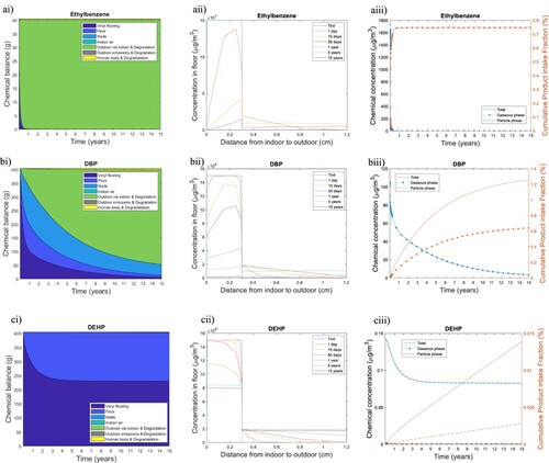
Ethylbenzene is entirely emitted from the vinyl flooring to the outdoor, via volatilization to indoor air over the first year (Figure 1(ai)). Ethylbenzene mass in the vinyl flooring decreases by a factor 5 in only 15 days (Figure 1(aii)). A fraction of ethylbenzene sorbs onto the walls for the first few days (ethylbenzene concentration reaches 5 × 10⁷ µg m⁻³ in the painting layer one day after vinyl flooring’s installation) but desorbs really quickly (its concentration in the painting layer has already decreased to 2 × 10⁶ µg m⁻³ after 50 days) and is then ventilated to outdoor air. The desorption can be explained by a lower indoor air concentration, and therefore the concentration gradient has been reversed. As a result, ethylbenzene concentration in the gaseous phase is almost zero after 200 days. A negligible ethylbenzene mass is emitted directly outdoors after diffusion from the bottom of vinyl flooring through the concrete underneath. Ethylbenzene emission dynamics is governed by its high diffusion coefficient ($D_m$ = 3 × 10⁻¹² m² s⁻¹) and its low material-air partition coefficient ($K_{ma}$ = 4 × 10³), which makes this chemical diffuse quickly within the vinyl flooring and be rapidly transferred from the solid phase to the air, once it has reached the vinyl flooring surface. The human intake of ethylbenzene represents almost 1% of its initial mass (Figure 1(aiii)), with inhalation as the main intake route.

In contrast, only 0.4% of DEHP initial mass has been released after 15 years (Figure 1(ci)). DEHP’s material-air partition coefficient is high ($K_{ma}$ = 6 × 10¹⁰), meaning that it is difficult for this chemical to leave the solid phase. Therefore, DEHP preferentially diffuses into the other layers of the floor, principally in the concrete, thus the importance to consider these different layers. After three years, the mass transfer between the vinyl and the concrete layer reaches an equilibrium: the DEHP flow from vinyl to concrete is the same as the flow from concrete to vinyl. The high value of $K_{ma}$ also implies that the small fraction of DEHP volatilized tends to continuously sorbs to the surface of the sidewalls. Once DEHP has sorbed on the painting layer of the wall, it also preferentially diffuses into the other layers of the wall than desorbs. DEHP diffuses through the painting layer and the gypsum board; however, DEHP mass is negligible within insulation layers. Almost all the DEHP mass in the gaseous phase is sorbed to particles (Figure 1(biii)) due to a very high particle-air partition coefficient $K_{pa}$.

DPB represents an intermediary situation: Almost half of DBP has been emitted over the first year, but at the end of the flooring lifetime DBP has not been emitted entirely, and 1% of its initial mass is still present in the vinyl flooring and 2% has migrated in the other layers of the floor (mainly slab) (Figure 1(bi)). Sorption is an important removal pathway for DBP: the mass balance shows that on average over 15 years, 9% of its initial mass is sorbed into the ceiling and walls. DBP adsorbs to the walls and ceiling quickly during the first 100 days, but then the sorption rate is slowed down until DBP starts to desorb from the walls and the ceiling 200 days later. At the end of the 15 years lifetime, half of the DBP sorbed into the walls is contained in the gypsum layer, one-third in the insulation layers of the walls and 15% in the painting. DBP has a diffusion coefficient one order of magnitude smaller than that of ethylbenzene but similar to DEHP ($D_m$ = 3 × 10⁻¹³ m² s⁻¹ for DBP and $D_m$ = 1 × 10⁻¹³ m² s⁻¹ for DEHP). However, its partition coefficient is 4 order of magnitude smaller than DEHP which explains that the dynamic of emission of DBP is steeply faster than DEHP.

Since DBP is emitted and then desorbs over vinyl-flooring lifetime, occupants are consequently exposed to this phthalate over the first 10 years mainly through inhalation (contributes to 50% of the total intake) and dermal gaseous uptake (other 50% of the total intake: Figure 1(biii)). Indeed, dermal gaseous uptake turns out to be a significant exposure pathway for chemicals with:

• a high material-air partition coefficient, because the dermal gaseous uptake is directly proportional to the gaseous skin permeation coefficient, which depends on the same chemical properties as $K_{ma}$

• a relatively high emission rate: indoor air concentration should be relatively high compared to the dust concentration at the flooring surface.

3.2. Effect of temperature on the dynamics of emission, indoor fate and human exposure

Sensitivity study: Since emission and sorption dynamics of DEHP, DBP and ethylbenzene differ substantially as a function of their respective diffusion and material-air partition coefficients at standard temperature, this section aims at studying the sensitivity of their emission and fate to temperature.

We therefore first explore how these two parameters driving chemical emission evolve with temperature. The relationship between the temperature and $D_m$ and $K_{ma}$ established by Huang et al. (2017b; Huang and Jolliet 2018) shows that when temperature increases, $D_m$ increases while $K_{ma}$ decreases as illustrated in Figures 2(a,b), respectively. Temperature variation from 25°C affects substantially $K_{ma}$ in low-temperature ranges and $D_m$ in high-temperature ranges. The variation of $K_{ma}$ with temperature only depends on the chemical enthalpy of vapourization ($\mathrm{\Delta }{H}_v$), whereas, $D_m$ variation with temperature also depends on material type.

Figure 2. Relative evolution of the (a) diffusion coefficient, (b) material-air, (c) material-water and (d) particle-air partition coefficients over their respective value at the standard temperature T_std of 25°C. ΔH_v (kJ·mol⁻¹) refers to the enthalpy of vapourization, τ is a material-dependent coefficient for estimating the diffusion coefficient (for example, τ = 2391 for polystyrene, τ = 1676 for polyurethane foam based material and τ = 0 for cement).

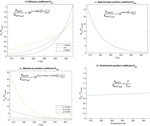
In addition, temperature variation is likely to modify the relative contribution of the different exposure pathways to total exposure. When temperature rises, the partition between the gaseous and particulate phase increases very slightly (Figure 2(d)), slightly reducing the proportion of chemical susceptible to sorb from the gaseous phase onto the epidermis. However, the partition between the gaseous phase and the skin significantly increases (Figure 2(c)), likely to increase the relative contribution of gaseous dermal uptake to total exposure compared to inhalation.

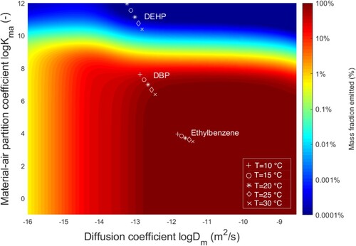
Figure 3 presents the mass fraction emitted over 15 years from a 0.3 mm-thick vinyl flooring for all $D_m$ and $K_{ma}$ combinations expected to cover most of common chemicals in this material. Slow internal diffusion (i.e. low $D_m$ – left of Figure 3) or strong affinity to the building material (i.e. high $K_{ma}$ – upper part of Figure 3, such as DEHP) limits chemical releases, leading to low mass fractions emitted. In contrast, 99% of the initial mass of chemical is emitted over 15 years, for chemicals such as ethylbenzene, with a diffusion coefficient higher than 2 × 10⁻¹³ m² s⁻¹ and a partition coefficient smaller than 4 × 10⁶. Figure 3 uses differentiated markers to illustrate for ethylbenzene, DBP and DEHP the effect of temperature variations from 10°C to 30°C on $D_m$, $K_{ma}$ and the resulting fraction emitted. $D_m$ varies in the same range for the three chemicals (less than one order of magnitude) since its variation only depends on the materials’ properties as previously seen (vinyl flooring). Ethylbenzene material-air partition varies in the same range as its diffusion. However, $K_{ma}$ varies by two orders of magnitude for DEHP and DBP when the temperature shifts from 10°C to 30°C. This higher variation than for ethylbenzene can be explained by the high enthalpy of vapourization of DEHP and DBP ($\mathrm{\Delta }{H}_v$ = 106 kJ mol⁻¹ and $\mathrm{\Delta }{H}_v$ = 85 kJ mol⁻¹, respectively, against $\mathrm{\Delta }{H}_v$ = 39 kJ mol⁻¹ for Ethylbenzene). Such a variation is crucial in affecting DBP and DEHP’s emission dynamics since, as previously seen, $K_{ma}$ is the limiting factor to the release of both chemicals.

Figure 3. Mass fraction emitted over 15 years as a function of the diffusion $D_m$ and material-air partition $K_{ma}$ coefficients at different temperatures T.

As a result of this decrease in $K_{ma}$, the mass fraction volatilized at the surface of the vinyl flooring increases with temperature. Four hundred twenty-two days are needed to emit 99% of ethylbenzene at 10°C, whereas only 160 days are required to reach this level at 30°C. The increase in volatilization is even larger for DBP and DEHP than for ethylbenzene because of the stronger decrease in $K_{ma}$ for phthalates due to their high enthalpy of vapourization. A factor 8 higher mass fraction of DEHP and DBP has been emitted over one year at 30°C (0.08% and 8%, respectively) than at 10°C (0.01% and 1% respectively). Since the increase in $K_{ma}$ is higher in the low temperature range (Figure 2(b)), the increase in mass fraction emitted is more important between 10°C and 15°C (+46% over the first year for DBP) than between 25°C and 30°C (+13% over the first year for DBP).

A higher temperature speeds up emission dynamics, and also results in a higher peak concentration in the indoor air for the three chemicals, with increases in maximum concentration of ethylbenzene, DBP and DEHP by a factor 2, 20 and 35 from 10°C to 30°C, respectively (Figure S2(a)). Only the short-term dynamic of ethylbenzene is impacted by the temperature since its emission dynamics is rapid and all of the ethylbenzene is anyway emitted from the vinyl flooring after one year. As a result, the mean indoor air concentration of ethylbenzene over the first year is independent of temperature. The slower the emission dynamics, the higher the influence of temperature on the mean concentration increase: the mean concentration of DBP and DEHP over the vinyl flooring lifetime increases by a factor of 4 and 35 times, respectively, from 10°C to 30°C (Figure S2(b,c)).

Decreases in $K_{ma}$ also mean that it is harder to sorb onto the walls once the chemical is released into the indoor air. As a result, DBP concentration on walls surfaces decreases when temperature increases.

For DBP and ethylbenzene, the sums of all exposure pathways $PiF$ are directly proportional to this mean indoor air concentration since inhalation and gaseous dermal uptake are the major exposure pathways to both chemicals. Thus, the $PiF$ for ethylbenzene over 15 years remains the same regardless of the temperature (Figure S3(a)), whereas for DBP, the $PiF$ is four times higher at 30°C than at 10°C (Figure S3(b)).

On the contrary, DEHP $PiF$ is entirely driven by dust ingestion at 10°C (Figure S3(c)) and is proportional to the mean concentration at the vinyl flooring surface. Since the surface concentration decreases when temperature increases, the mass of DEHP taken in via ingestion over the first year slightly decreases from 10°C to 30°C. Since, DEHP indoor concentration increases between 10°C and 30°C, the contribution of the dermal gaseous uptake pathway to total exposure becomes more important for higher temperature.

We carried out a sensitivity study on 63 SVOCs and VOCs commonly found in vinyl floorings, varying temperature between 10°C and 30°C. Table S4 shows that over the flooring lifetime (15 years), average indoor air concentration at 30°C could be up to six times higher than at 10°C and PiF up to 3.5 times higher. The impact of temperature is substantial mostly for SVOCs. Since temperature does not affect ingestion pathway via dust while it does for inhalation and gaseous exposure pathway, PiF increase might be less important than indoor air concentration increase.

Annual and daily evolution of indoor concentrations, exposures and consumption as a function of climate: By consistently coupling heat and mass transfer equation, our model enables us to study the incidence of local climate and related temperature on indoor air exposures. Figure 4(a) shows the evolution of indoor and outdoor air temperatures over a full year for a continental climate (Lille, France) and its climate analogue in 2050 (Nice, France). In a climate change context, indoor temperature during winter time is maintained to its setpoint by heating devices. However, during summer, indoor temperature is not controlled for the majority of European household (for example, the French Environment and Energy Agency reported that a quarter of French households are equipped with air conditioning (CODA Stratégies, ADEME 2021)). This means that in house without air conditioning, indoor air temperature maximum and mean values are likely to rise in the coming years. Besides, in air-conditioned houses, even if indoor air temperature is maintained at a setpoint, as external air temperature will be higher, the gradient of temperature within the building envelope will increase (the difference of temperature between the outermost layer of the building envelope and the innermost layer). To represent a standard case, no air conditioning has been designed during summer.

Figure 4. (a) Yearly evolution starting from 1st of January of indoor temperature (solid lines, y-left axis), outdoor temperature (dotted lines, y-left axis) and cumulative energy demand for a fixed heating duration from November 1st (day 280) to April 1st (day 140) (dashed lines, y-right axis) in Lille (blue colour), Nice (red colour) and for the standard scenario with 20°C outdoor constantly (black colour). The other sub-graphs represent indoor air concentration (solid lines, y-left axis) of (b) Ethylbenzene, (c) DBP and (d) DEHP, as well as cumulative Product intake Fraction (PiF) (dashed lines, y-right axis).

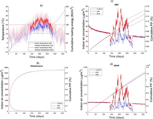
Figure 4(b–d) presents the evolution in indoor concentration of the three organics over the entire year. Ethylbenzene concentration does not vary as a function of the temperature, since 100% is emitted relatively rapidly. On the contrary, DBP and DEHP indoor air concentration vary with temperature, mostly during summer because of the strong dependence of $K_{ma}$ with temperature, with especially high summer concentrations in Nice for both DBP and DEHP. When considering cumulative exposures over the entire year, it is only for DEP that PiF and exposures increase by about 20% between Nice and Lille, due to the higher observed temperature during the summer period. These results demonstrate that the increase of temperature induced by climate change is likely to significantly increase occupants’ exposure to building materials’ emission.

In contrast, cumulative energy demand for heating the room over one year is 35% higher in Lille than in Nice (dashed lines in Figure 4(a)) since outdoor temperature in Lille are on average colder (dotted lines in Figure 4(a)). It should be noted that for a fair comparison, the number of heating days should a-priori be location dependent.

These results demonstrate that the increase of temperature induced by climate change is likely to significantly increase occupants’ exposure to building materials’ emission.

3.3. Impact of air renewal rate on heating load and indoor exposure to chemicals in building products

The combined heat and mass transfer model also enables us to inform early design choices and analyse influence of air renewal rates and trade-offs between heating load and air quality. The air renewal rate (entry data of the model) has been modified in this section from 0.3 to 1.3 h⁻¹. The air renewal rate impacts both energy demand for heating due to the intake of cold air from outside in winter (Equation 4(a)) and air quality by removing substance from indoor to outdoor (Equation 4(b)).

Figure 5 characterizes human exposure by presenting the PiF (left blue y-axis) and energy demand for heating (right green y-axis) as a function of the different air renewal rate. As illustrated in Figure 5, higher the air renewal rate, smaller the Product intake Fraction (PiF) over 15 years, particularly for pollutants with a fast emission dynamic (for example, as shown in Figure 5, Ethylbenzene PiF over 15 years decreases by 60% if air renewal rate is 1.2 vol h⁻¹ instead of 0.4 vol h⁻¹). Increasing the rate of air exchange means a smaller residence time of chemicals indoors but also an increase in chemical emission rate due to the increased concentration gradient. Substances with a fast emission dynamic are completely emitted from the material over its lifetime anyway (for example, Ethylbenzene has been completely emitted in less than one year), so an increase of the emission rate due to higher air exchange rate will not affect the mass that has been finally emitted. However, for pollutants with a smaller emission dynamic such as DEHP for which less than 1% of its initial mass has been released over the material lifetime, the higher emission rate almost counterbalances the smaller residence time indoors. Ethylbenzene PiF for Lille and Nice are almost the same over 15 years since this chemical is already entirely emitted after half a year, whatever indoor/outdoor temperature.

Figure 5. Energy loss by air renewal rate without (plain bar) and with (dotted bar) a heat exchanger and Product intake Fraction (PiF) of Ethylbenzene (dashed line), DBP (solid line) and DEPH (dotted line, its PiF values have been multiplied by 100 to appear at the same scale) in Lille (blue colour) and Nice (red colour) as a function of the air renewal rate, over 15 years.

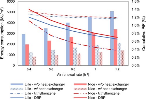
Heating load varies linearly as a function of the amount of cold air entering the building that should be heated up to the setpoint temperature. Note that the energy consumption related to the power that the air handling unit motor should deliver as a function of the supplied airflow has not been taken into account. Note also that change of airspeed due an increasing ventilation rate is not accounted for when calculating the indoor convection heat coefficients. Indeed, Fisher and Pedersen (1997) showed for example that for a ventilation of 6 vol h⁻¹, the daily calculated load on the system based on convective coefficient accounting for airspeed varies from 5% to the one based on simpler natural convection correlations. The air renewal rates under study are far smaller than that (from 0.4 to 1.3 vol h⁻¹) to represent typical residential environments (Rosenbaum et al. 2015). Thus, the influence of airspeed on the heat convective coefficient is expected to be negligible compared to the other uncertainties (for example, the internal radiative balance in short wave due to sun temperature is realized with the hypothesis that the solar flux entering the room through the window only touches the floor).

A reasonable compromise for which both indoor exposure and heating load are relatively low, is for a ventilation rate of 0.6 ACH (air change per hour) above which the reduction in chemical exposure becomes restricted. The installation of the heat exchanger (efficiency of 0.7, described in Section S5 of SI) allows reducing the heating load for the same air renewal rate and level of human exposure. Warm indoor air, which has been heated up indoors until the temperature setpoint, go out through the plates in the heat exchange, designed to optimize the convective heat transfer between the warm indoor air and the cold outdoor air. This way, the cold air coming from outdoor is heated before it reaches the indoor environment. For example, with a ventilation rate of 0.6 ACH, the heating load is reduced by 40% when a heat exchanger is installed, potentially enabling to slightly increase ventilation while keeping heat losses restricted.

During summer, for buildings with high thermal inertia, cooling at night using natural ventilation ensures improved thermal comfort during the day. This could then contribute to reduce peak concentrations during the day in offices for example. In addition to its dilution function, ventilation increases the convective transfer coefficient at the surface of the material, so is the concentration gradient between the building materials and the indoor air.

On the other hand, exchanges with the outdoor potentially bring outdoor pollutants indoors, such as ozone or hydroxyl radicals, which can further react with organic compounds to form secondary organic pollutants unless filtered. This burden shifting should be further investigated as well as the potential installation of high-quality filters on indoor air recirculation that could reduce indoor exposures without additional heat losses.

4. Conclusion

We developed a unique dynamic model fully coupling heat and chemical mass transfer through the building envelope. It provides a better understanding of building materials as an indoor source of pollution by providing insight into the dependence of the emission and sorption process on temperature.

The impact of temperature on the fraction of pollutant initially contained in material that is uptake indoors by the human body over the material lifetime is substantial for SVOCs. On the contrary for VOCs, temperature impacts the short-term dynamics (increase of concentration peak) but not the intake fraction over the material lifetime mostly driven by the mean concentration of pollutants in the gaseous phase. The temperature increase due to climate change for a city like Lille (France) which will be located at the level of the climate of Nice (France) in 2050 (www.ccexplorer.eu) will increase the exposure of the occupants to the SVOC emissions of building materials by 20%. To maintain acceptable levels of occupant exposure in the coming years, the masses of chemicals used in building materials should therefore be lowered.

Using this model, design choices can be compared towards the resulting mass of chemicals taken in by the human body as well as the heating load. This approach paves the way for designing energy-efficient buildings that do not compromise occupants’ health, and the potential applications are manifold. For example, outer insulation has been generalized in the last decade because it increases the overall thermal performance of the building. The benefits of outer versus inner insulation in terms of indoor air quality should be also assessed in a routine way. As studied by Maury-Micolier et al. (2023), the impact of external insulation on chemical emission depends on the physico-chemical properties of chemicals under study. For pollutants with a fast diffusion in material, the position of the insulation does not affect substantially the mass of substance emitted indoors over the material lifetime, but it will affect the peak concentration. In contrast, less volatile substances do not migrate through the concrete layer if thick enough, and are entirely emitted inside with an inner insulation while entirely emitted outside with an outer insulation. Besides, some materials are selected for the importance of their latent heat at a given temperature level, and integrating this issue to guide material selection in building design constitutes an interesting research opportunity. The dynamic simulation proposed by this model is also a way forward to quantify the health risk resulting from the exposure to high but episodic chemical concentrations indoors.

Disclosure statement

No potential conflict of interest was reported by the author(s).

Data availability statement

The authors confirm that the data supporting the findings of this study are available within the article and its supplementary materials.

Additional information

Funding

The work at Technical university Denmark and University of Michigan has been partly supported by the United Nations Environment Programme (UNEP) in the frame of ‘Global Best Practices on Emerging Chemical Policy Issues of Concern under UN Environment’s Strategic Approach to International Chemicals Management (SAICM)’ (grant no. S1-32GFL-000632), and by the USEtox International Center at Technical University Denmark.

References

- Axley, J. W. July 1991. “Adsorption Modelling for Building Contaminant Dispersal Analysis.” Indoor Air 1: 147–171. doi:10.1111/j.1600-0668.1991.04-12.x.
- Beko, G., C. J. Weschler, S. Langer, M. Callesen, J. Toftum, and G. Clausen. 2013. “Children’s Phthalate Intakes and Resultant Cumulative Exposures Estimated from Urine Compared with Estimates from Dust Ingestion, Inhalation and Dermal Absorption in Their Homes and Daycare Centers.” PLoS One 8. doi:10.1371/journal.pone.0062442.
- ChemSpider. 2020. Accessed November 11, 2020. www.chemspider.com.
- Chickos, J. S., and W. E. Acree. June 2003. “Enthalpies of Vaporization of Organic and Organometallic Compounds, 1880–2002.” Journal of Physical and Chemical Reference Data 32: 519–878. doi:10.1063/1.1529214.
- Clausen, P. A., Y. Xu, V. Kofoed-Sørensen, J. C. Little, and P. Wolkoff. May 2007. “The Influence of Humidity on the Emission of Di-(2-ethylhexyl) Phthalate (DEHP) from Vinyl Flooring in the Emission Cell ‘FLEC’.” Atmospheric Environment 41: 3217–3224. https://linkinghub.elsevier.com/retrieve/pii/S1352231006011460. doi:10.1016/j.atmosenv.2006.06.063.
- CODA Stratégies, ADEME. 2021. La climatisation dans le bâtiment – Etat des lieux et prospective 2050. 59.
- De Bellis, L., F. Haghighat, and Y. Zhang. 1995. “Review of the Effect of Environmental Parameters on Material Emissions.” In: International Conference on Indoor Air Quality, Ventilation and Energy Conservation in Buildings, Montreak (Canada).
- Dols, W. S., and B. J. Polidoro. 2015. CONTAM User Guide and Program Documentation – Version 3.2 (NIST Technical Note 1887).
- EPA. 2011. Exposure Factors Handbook.
- Fantke, P., M. Bijster, C. Guignard, et al. 2017. USEtox® 2.0 Documentation.
- Feustel, H. E. 1998. COMIS – An International Multizone Air-Flow and Contaminant Transport Model.
- Fisher, D. E., and C. O. Pedersen. 1997. “Convective Heat Transfer in Building Energy and Thermal Load Calculations.” ASHRAE Transactions 103: 137–148.
- Gaspar, F. W., R. Castorina, R. L. Maddalena, M. G. Nishioka, T. E. McKone, and A. Bradman. 2014. “Phthalate Exposure and Risk Assessment in California Child Care Facilities.” Environmental Science & Technology 48: 7593–7601. doi:10.1021/es501189t.
- Guo, Z. 2013. “A Framework for Modelling Non-Steady-State Concentrations of Semivolatile Organic Compounds Indoors: Emissions from Diffusional Sources and Sorption by Interior Surfaces.” Indoor and Built Environment, 685–700. doi:10.1177/1420326X13488123.
- Haghighat, F., and L. De Bellis. 1998. “Material Emission Rates: Literature Review, and the Impact of Indoor air Temperature and Relative Humidity.” Building and Environment 33: 261–277. doi:10.1016/S0360-1323(97)00060-7.
- Harish V. S. K. V., and A. Kumar. 2016. “A Review on Modeling and Simulation of Building Energy Systems.” Renewable & Sustainable Energy Reviews 56: 1272–1292. doi:10.1016/j.rser.2015.12.040.
- HBN Healthy Building Network. 2020. The Pharos Project. 2020. Accessed November 11, 2020. http://pharosproject.net.
- Huang, L., A. Ernstoff, P. Fantke, S. A. Csiszar, and O. Jolliet. 2017a. “A Review of Models for Near-Field Exposure Pathways of Chemicals in Consumer Products.” Science of the Total Environment 574, 1182-1208. doi:10.1016/j.scitotenv.2016.06.118.
- Huang, L., P. Fantke, A. Ernstoff, and O. Jolliet. 2017b. “A Quantitative Property-Property Relationship for the Internal Diffusion Coefficients of Organic Compounds in Solid Materials.” Indoor Air 27: 1128–1140. doi:10.1111/ina.12395.
- Huang, L., and O. Jolliet. 2018. “A Quantitative Structure-Property Relationship (QSPR) for Estimating Solid Material-Air Partition Coefficients of Organic Compounds.” Indoor Air, 0–2. doi:10.1111/ina.12510.
- Huang, L., A. Micolier, H. P. Gavin, and O. Jolliet. August 25, 2021. “Modeling Chemical Releases from Building Materials: The Search for Extended Validity Domain and Parsimony.” Building Simulation 14: 1277–1293. doi:10.1007/s12273-020-0739-6.
- Hunt, D., and M. Gidman. 1982. “A National Field Survey of House Temperatures.” Building and Environment 17: 107–124. doi:10.1016/0360-1323(82)90048-8.
- Jolliet, O., A. S. Ernstoff, S. A. Csiszar, and P. Fantke. 2015. “Defining Product Intake Fraction to Quantify and Compare Exposure to Consumer Products.” Environmental Science & Technology 49: 8924–8931. doi:10.1021/acs.est.5b01083.
- Klepeis, N. E., W. C. Nelson, W. R. Ott, et al. 2001. “The National Human Activity Pattern Survey (NHAPS): A Resource for Assessing Exposure to Environmental Pollutants.” Journal of Exposure Science & Environmental Epidemiology 11: 231–252. doi:10.1038/sj.jea.7500165.
- Liang, Y., and Y. Xu. 2014. “Emission of Phthalates and Phthalate Alternatives from Vinyl Flooring and Crib Mattress Covers: The Influence of Temperature.” Environmental Science & Technology 48: 14228–14237. doi:10.1021/es504801x.
- Little, J. C., A. T. Hodgson, and A. J. Gadgil. January 1994. “Modeling Emissions of Volatile Organic Compounds from new Carpets.” Atmospheric Environment 28: 227–234. doi:10.1016/1352-2310(94)90097-3.
- Little, J. C., C. J. Weschler, W. W. Nazaroff, Z. Liu, and E. A. Cohen Hubal. October 16, 2012. “Rapid Methods to Estimate Potential Exposure to Semivolatile Organic Compounds in the Indoor Environment.” Environmental Science & Technology 46: 11171–11178. doi:10.1021/es301088a.
- Macintosh, D. L., T. Minegishi, M. A. Fragala, J. G. Allen, K. M. Coghlan, and J. H. Stewart. 2012. “Mitigation of Building-Related Polychlorinated Biphenyls in Indoor Air of a School.” Environmental Health, 1–10. doi:10.1186/1476-069X-11-24.
- Maury-Micolier, A., L. Huang, F. Taillandier, G. Sonnemann, and O. Jolliet. 2023. “A Life Cycle Approach to Indoor Air Quality in Designing Sustainable Buildings: Human Health Impacts of Three Inner and Outer Insulations.” Building and Environment 230. doi:10.1016/j.buildenv.2023.109994.
- Meteonorm. 2009. https://meteonorm.meteotest.ch/en/meteonorm-timeseries.
- Météo France. 2020. Accessed November 11, 2020. https://donneespubliques.meteofrance.fr.
- Myers, G. E. 1985. “The Effects of Temperature and Humidity on Formaldehyde Emission from UF-Bonded Boards: A Literature Critique.” Forest Products Journal 35: 20–31. https://www.fpl.fs.usda.gov/documnts/pdf1985/myers85a.pdf.
- NF ISO 16000-6. 2012. Determination of Volatile Organic Compounds in Indoor and Test Chamber Air by Active Sampling on Tenax TA® Sorbent, Thermal Desorption and Gas Chromatography Using MS or MS-FID.
- Ouyang, K., and F. Haghighat. 1991. “A Procedure for Calculating Thermal Response Factors of Multi-Layer Walls-State Space Method.” Building and Environment 26: 173–177. doi:10.1016/0360-1323(91)90024-6
- Peeters, L., I. Beausoleil-Morrison, and A. Novoselac. 2011. “Internal Convective Heat Transfer Modeling: Critical Review and Discussion of Experimentally Derived Correlations.” Energy and Buildings 43: 2227–2239. doi:10.1016/j.enbuild.2011.05.002.
- Pilka, T., I. Petrovicova, B. Kolena, T. Zatko, and T. Trnovec. 2014. “Relationship Between Variation of Seasonal Temperature and Extent of Occupational Exposure to Phthalates.” Environmental Science and Pollution Research 22: 434–440. doi:10.1007/s11356-014-3385-7.
- Rosenbaum, R. K., A. Meijer, E. Demou, et al. 2015. “Indoor Air Pollutant Exposure for Life Cycle Assessment: Regional Health Impact Factors for Households.” Environmental Science and Technology 49: 12823–12831. doi:10.1021/acs.est.5b00890.
- Stewart, J., and Z. Ren. December 2006. “COwZ – A Subzonal Indoor Airflow, Temperature and Contaminant Dispersion Model.” Building and Environment 41: 1631–1648. doi:10.1016/j.buildenv.2005.06.015.
- US Department of Energy. 2010. EnergyPlus Engineering Reference: The Reference to EnergyPlus Calculations.
- Walton, G. 1983. Thermal Analysis Research Program (TARP) Reference Manual. National B. Washington, DC.
- Wei, W., C. Mandin, and O. Ramalho. March 2018. “Influence of Indoor Environmental Factors on Mass Transfer Parameters and Concentrations of Semi-Volatile Organic Compounds.” Chemosphere 195: 223–235. doi:10.1016/j.chemosphere.2017.12.072
- Wei, W., O. Ramalho, and C. Mandin. 2019. “A Long-Term Dynamic Model for Predicting the Concentration ofSemivolatile Organic Compounds in Indoor Environments: Application to Phthalates.” Building and Environment 148: 11–19. doi:10.1016/j.buildenv.2018.10.044.
- Yan, W., Y. Zhang, and X. Wang. 2009. “Simulation of VOC Emissions from Building Materials by Using the State-Space Method.” Building and Environment 44: 471–478. doi:10.1016/j.buildenv.2008.04.011.