An ensemble-based faults detection and diagnosis approach for determining faults severities at whole-building level

Abstract

Data-driven fault detection and diagnosis (FDD) approaches rely on operational data even when in-depth knowledge of the studied system is lacking. Simulated data is affordable and can cover numerous fault types and severities. Developing FDD models with a single fault severity has limitations on the model's generalisability owing to evolution of faults with severities. Thus, machine learning models must be individually trained on diverse scenarios. Current studies on building FDD are often at system levels, thereby leaving significant knowledge gaps when there is interest in energy performance of an entire building. This research presents a data-driven FDD approach for classifying several building faults using different ensemble multi-class classification approaches. Additionally, the impact of noise on training datasets is investigated. The XGBoost classifier achieved the highest classification accuracy for the considered faults during validation and testing stages, with low sensitivity to noise, thereby demonstrating a promising potential for wider scale deployment.

KEYWORDS:

• Building energy performance
• building maintenance
• fault detection and diagnosis (FDD)
• ensemble learning
• multi-class classification

1. Introduction

Energy conservation and carbon emission regulations are increasing globally in response to the ever-growing energy crisis and climate change. Various nations and regions have established their reaction plans. For instance, the European Parliament passed the European Climate Law, which increases the EU's 2030 emission reduction goal to at least 55% from 40% and imposes a legal obligation for all countries to achieve climate neutrality by the year 2050 (European Parliament 2019). Despite being among the largest oil producers, Saudi Arabia intends to reach net zero emissions by 2060 through its newly enacted Carbon Circular Economy strategy (SGI 2021). Buildings and building construction sectors account for nearly one-third of total global energy consumption and 15% of direct carbon dioxide (CO₂) emissions (International Energy Agency 2022). Thus, substantial efforts and initiatives have been applied internationally to improve buildings’ energy efficiency, particularly with the increase in the global population rate.

Ensuring that building systems are in good condition is one aspect that enhances a building's energy performance since it is equipped with various types of systems and a malfunction in any of these systems could lead to excessive energy wastage and an increase in carbon emissions. An assessment of UK’s buildings has revealed that 25–50% of energy is wasted due to faults in heating ventilation air conditioning (HVAC) systems (Yu, Woradechjumroen, and Yu 2014). This wastage could be reduced to less than 15% if those faults could be detected at their incipient stages, which could help avert incurring undesirable expenses (Yu, Woradechjumroen, and Yu 2014).

1.1. Overview of the maintenance strategies

In general, maintenance strategies can be categorized as reactive maintenance (RM), planned preventive maintenance (PPM), and predictive or condition-based maintenance (CBM) (Alghanmi, Yunusa-kaltungo, and Edwards 2022; Yunusa-Kaltungo, Kermani, and Labib 2017; Yunusa-Kaltungo and Labib 2021). The RM class of maintenance strategies represents maintenance interventions that are initiated only when a failure or breakdown has occurred. RM is considered the first-generation maintenance strategy, which was dominant when materials were abundant and very little competition amongst service providers. However, the high cost of downtime associated with RM triggered the initiation of alternative maintenance strategies, including PPM whereby asset owners initiate maintenance interventions based on time, irrespective of the state of health of the asset. Examples of PPM include periodic replacements of components such as HVAC filters, strictly based on a calendar schedule and not their conditions. Although PPM reduced the wastage associated with RM, it wasn’t still considered optimum, because fit-for-purpose components are sometimes replaced. Hence, CBM was introduced, whereby the assets themselves dictate their maintenance intervals through routinely monitored operational parameters such as temperature, humidity, airflow, pressure, etc. Despite the potency of CBM, it must be noted that it is best reserved for only critical assets, so as to strike a good balance between the efforts invested and the returned benefits. Therefore, an all-encompassing maintenance policy should integrate all strategies, whereby RM is dedicated to less critical assets, PPM to critical assets that do not have parameters that can be measured and CBM to critical assets that have measurable parameters.

Just as is the case with physical industrial assets (PIAs) within heavy duty industries, buildings also have some acceptable strategies for regular manual maintenance, such as PPM or RM but due to aforementioned reasons, especially increased equipment downtime cost, deterioration, and spare parts planning times (Ayu and Yunusa-Kaltungo 2020; Yunusa-Kaltungo and Sinha 2017), this may not be the most cost effective method for all buildings and their associated systems.

1.2. Overview of the fault detection and diagnosis (FDD) approaches

FDD technology (a subset of CBM) is a quicker, more sensitive, and possibly less expensive option for providing anomaly detection and health management (Zhu et al. 2019). Consequently, it may be considered to be an effective and reliable approach for managing the operational risk of building systems. FDD techniques may be broadly divided into three groups: data-driven (McHugh, Isakson, and Nagy 2019; Yun, Hong, and Seo 2021), model-based (Andriamamonjy, Saelens, and Klein 2018; Gao et al. 2016), and rule-based (Guo et al. 2019). The data-driven (‘black-box’) strategy is completely reliant on operational history, requiring a vast amount of historical data. It establishes a relationship between the recorded input and recorded output data of a process or system, but it does not need any physical understanding or background of the studied system (Tran, Chen, and Jiang 2016). Several researchers have reported the implementation of data-driven FDD approaches in the building sector, including Alghanmi, Yunusa-Kaltungo, and Edwards (2021), who explored the performance of several types of algorithms, including the isolation forest, the one-class support vector machine (OC-SVM), and the LSTM-autoencoder, on the identification of package air conditioning unit faults using limited data. As a result, the LSTM- autoencoder offered the best fault detection performance of all other techniques with an average precision rate of about 80%. In a similar manner, Fan et al. (2021) developed a semi-supervised neural network to diagnose air handling unit (AHU) faults including air dampers and heating/cooling coil valves stuck as well as fan speed stagnation using limited labelled data. Consequently, the heating and cooling coil valve failures were more easily identified, with typical recall rates of around 92.74% and 73.64%, respectively. Other faults, on the other hand, were difficult to identify without label data; for example, an outside air damper stuck fault had an average recall of only 12.82%.

Han et al. (2020) utilized K-nearest neighbour (KNN), SVM, and random forest (RF) as ensemble members to diagnose various centrifugal chiller faults such as refrigerant leak/undercharge and condenser fouling. After parameters optimization, the conventional approaches were incorporated into an ensemble diagnostic model (EDM) via the majority voting approach. In comparison to the performance of the other three members, the ensemble EDM recorded the highest overall diagnostic accuracy of 99.88%.

The model-based strategy, on the other hand, can be described as either a white-box that is exclusively physical-based or a grey-box that encompasses both the black-box method that is completely data-driven and the white-box technique (Alexandersen et al. 2019; Zhao et al. 2019). Whereas, the rule-based method combines and analyses incoming sensor data in line with the pre-established set of rules to build a risk profile and triggers a reaction when the rules are broken (Schein et al. 2006). The study by Ahn, Mitchell, and McIntosh (2001) is an example of using a white-box method to detect and diagnose cooling tower circuit faults including water temperature sensors, water pump, and cooling fan. The detection and diagnosis were accomplished through the differences between the baseline and faulty conditions of the system's parameters, which included the temperature effectiveness, the conductance-area product, the fan power, and the temperature difference between the water leaving the tower and the entering air wet bulb temperature. Nevertheless, because the white box model uses complicated mathematical equations to represent the systems, it takes a considerable amount of computing resources. As a result, the grey box model has been used as an alternative to address this problem by using regression techniques for estimating the models’ parameters based on measured data (Singh, Mathur, and Bhatia 2022). As an example, Sun et al. (2017) developed a fault detection approach for an underground heat pump system to identify both sudden faults (pipe frozen) and gradual faults (pipe water leakage) by using a Kalman filter based on the grey model and the real system data to estimate the model parameters and its standards variance. Besides that, statistical process control (SPC) is used to build a dynamic control threshold to eliminate false alarms triggered by outside weather variations.

On the other hand, it is envisaged that a combination of different approaches (also known as hybridization whereby the strengths of one technique compensates for the limitations of others) may offer improved overall performance when compared to that obtainable via individualized models. This has been shown in the study conducted by Wei et al. (2022), who combined rule-based and model-based approaches to diagnose variable air volume (VAV) system faults by primarily utilizing mixed residual, qualitative, and quantitative methodologies. The quantitative fault model and the qualitative knowledge rules successfully matched faults and the obtained correlation coefficients between the fault model and the measured data were all more than 0.85.

Even though the model-based and rule-based methods performed well, they required numerous in-depth features, such as flow rates, temperatures, pressures, and so on, to generate mathematical representation models and required expert input to create diagnostic rules. Thus, the data-driven technique is popular and looks to be a more efficient alternative because it does not need a deep system background; however, it does necessitate a large quantity of training data. This popularity might be attributed to the fact that most buildings are becoming increasingly data-intensive, particularly in relation to the availability of building energy management systems (BEMS) and the developing trend of deep learning algorithms. The performance of the deployed data-driven FDD techniques is heavily reliant on the quality and quantity of operational data that reflects both healthy and faulty operations, which is comparatively rare (Ebrahimifakhar, Kabirikopaei, and Yuill 2020). Thus, this challenge may have to be tackled in the building sector by employing simulation software such as EnergyPlus (Gunay et al. 2018), TRNSYS (Bin Yang et al. 2014) and MATLAB/Simulink (Shohet, Kandil, and McArthur 2019) to generate ample operational data for buildings, which adequately mimic real-life system malfunctions to acquire faulty data with less noise, since the collected real data usually comes with an appreciable degree of noise or incompleteness which might lead to misclassification issue.

Depending on the labelling of the training dataset, the data-driven diagnosis approach can be used as supervised or unsupervised learning technique. With labelled dataset, supervised multi-class classification approaches are better suited for handling fault classification tasks (Li et al. 2021), especially neural network-based, tree-based, and SVM classifiers. A recent study by Shohet et al. (2020) investigated the performance of different supervised classification methods, including KNN, decision tree (DT), RF and SVM, for diagnosing various non-condensing boiler faults. The DT, RF and SVM methods recorded greater than 95% classification accuracies. Another study conducted by Zhou et al. (2020) was based on a comparison of different classification approaches, such as DT, SVM, shallow neural networks (SNN), deep neural networks (DNN), and a clustering approach. These were used to diagnose either single or multiple faults of variable refrigerant flow systems. The SVM, SNN, and DNN algorithms all outperformed the clustering algorithm. Furthermore, the overall correct diagnosis rate for multiple failures was lower than the rate for single fault diagnosis.

Building FDD analysis can be categorized in terms of the scope of the study into three levels of classification: system level, whole-building level, or multi-level framework (Yan et al. 2015). The whole-building scale assesses the building's energy consumption, such as electricity and gas to determine how effectively the building and its systems perform, resulting in a comprehensive view of the entire building's behaviour, rather than just a single system or component. Most of the previous works that have recently performed the whole-building analysis were in the field of fault detection such as (Lin and Claridge 2015) which identifies abnormal energy usage in educational buildings using a temperature-based approach known as the Days Exceeding Threshold. Another work by (Piscitelli et al. 2021) utilized a non-autoregressive multi-layer perception ANN in conjunction with a regression tree to build fault-free prediction (baseline) and compared it with the actual performance to detect any anomalous consumption in an educational building by using the entire building substation's electric usage. Also, (Mavromatidis, Acha, and Shah 2013) used the same concept of fault-free prediction using ANN-Levenberg – Marquardt to detect abnormal energy consumption in a commercial building. In terms of fault diagnosis, reference (Chen and Wen 2018) identified faults at the whole-building level in an educational building using principal component analysis (PCA), including chiller and AHU failures, and diagnose the identified fault using Bayesian networks (BNs). To the best of the authors’ knowledge, no research has been performed at the whole level employing a multi-class classification technique for detecting and categorizing operational faults with various severities. Furthermore, all of the above analyses were performed on educational and commercial buildings and the analysis of religious buildings is still underrepresented. This view is supported by the authors’ systematic review article (Alghanmi, Yunusa-kaltungo, and Edwards 2022) which found that no article analysed religious buildings, such as mosques and churches despite the huge number of such buildings and the enormity of the consequences of their operations on global energy consumption.

1.3. Utilization of ensemble classifiers in FDD

Besides the lack of generalisability of single-fault classification models, they have been reported to depict poor classification performance levels, especially when dealing with dynamic faults. As a consequence, several models may need to be integrated in various ways to form an ensemble model. The ensemble, also known as a multiple classifier or committee, is a collection of individual component classifier predictions that are aggregated to predict potential instances. They have been demonstrated to be an effective method of increasing prediction accuracy (Krawczyk et al. 2017). Popular examples of ensemble learning algorithms include bootstrap aggregations (bagging), weighted averages, and layered generalizations (stacking) (Patrick Schneider 2022). Recently, ensemble classifiers have been utilized to diagnose building faults to improve the single classification approaches. Table 1 presents different examples in the literature related to the implementation of the different ensemble algorithms in the detection and diagnosis of system faults within buildings.

Table 1. Summary of previous studies on ensemble approaches for detecting and diagnosing building system faults.

Reference	Approach	System	Faults	Severity
(Han et al. 2020)	Majority voting [consists of KNN, SVM, RF]	Centrifugal chiller system	Reduced evaporator water flow Reduced condenser water flow Refrigerant overcharge Refrigerant leakage Condenser fouling Non-condensable gas Excess oil	Single
(Yao, Li, and Gao 2022)	XGBoost, RF, LightGBM	Chiller	Reduced condenser water flow Reduced evaporator water flow Refrigerant leakage Refrigerant overcharge Excess oil Condenser fouling Non-condensable gas	Multiple
(Chakraborty and Elzarka 2019)	XGBoost	Water-cooled centrifugal chiller Packaged A/C unit VAV	Coefficient of performance reduction VAV motor efficiency and fan total efficiency reduction	Single
(Ebrahimifakhar, Kabirikopaei, and Yuill 2020)	Bagging, AdaBoost, XGBoost	Packaged A/C unit	Refrigerant undercharge Refrigerant overcharge Compressor valve leakage Liquid-line restriction Condenser airflow reduction Evaporator airflow reduction Non-condensable gas	Single
(McHugh, Isakson, and Nagy 2019)	Bagged Trees, Gradient Boosted Trees, AdaBoost Trees	Air handling unit (AHU)	Steam and chilled water valve leakage	Multiple

1.4. Overview of the addressed issues

The diagnostic effectiveness is greatly decreased when there is a variance between the actual diagnosis objective and the training dataset. In reality, the severity of a real building system’s failure, particularly an HVAC system, varies, and normally no two systems with the same sort of failure have the same severity. Also, the labelled data acquisition cost of the building's systems is very high, and it is impossible to collect enough labelled data for the evolution of the severity of each fault, thereby necessitating the employment of simulation tools under this circumstance.

Furthermore, some buildings lack a BEMS system, resulting in a limited range of feature sets that may not be sufficient to carry out whole-building fault detection/diagnosis work. Thus it is vital to investigate the capabilities of the data-driven FDD technique with limited training features. Besides the diagnostic accuracy of adopting FDD techniques, computational efficacy also needs to be investigated as it affects downtime or misoperation, which correlates significantly with the overall operational cost.

1.5. The contributions of this study

The goal of this research is to explore the effectiveness of ensemble-based classifiers in detecting and segregating various types of faults with different severities and to investigate the performance of classifying the severity of the diagnosed fault at the whole-building level with limited feature types and minimum running time.

The novelty of this research can be viewed from three aspects. Firstly, a whole-building faults diagnosis was performed on a religious building (a mosque) that had numerous systems faults with different severities due to the unique operational features of this type of building (varying occupancy across prayer times and days of the week). Secondly, the FDD study was carried out using only a few features extracted from the modelled energy usage readings and weather data. Thirdly, energy consumption statistical decomposition components were utilized on whole-building FDD, aiming to enhance the model classification performance.

The remainder of this study is organized as follows: Section 2 briefly discusses the multi-class classification techniques adopted for this research, including single and ensemble approaches, while Section 3 outlines the methodology of the research, as well as describing the case study building, and the introduced faults. Section 4 discusses the study findings and results in detail. Finally, Section 5 concludes the study.

2. Background

The fundamental idea behind the ensemble-based approaches is that there is power in unity. More effective models can be produced by combining various techniques, each of which has advantages and disadvantages. This necessitates choosing how to develop the ensemble’s models and how to aggregate the ensemble members’ predictions. The use of ensemble learning can help stochastic learning algorithms be more predictable and have lower variation (Patrick Schneider 2022). The following subsections provide a brief description of the applied approaches, including stacking with combined weak models and RF and boosting approaches.

2.1. Stacking classifier (SKC)

A stacking classifier is an ensemble technique that aggregates the results from various base classifiers to enhance predictive accuracy. It consists of a meta-classifier and base classifiers. Each base classifier is individually trained using a separate learning method to achieve the target task. The meta-classifier is trained to integrate the different strengths of different base classifiers by evaluating which base classifiers are more likely to be precise in accomplishing the target task for each class (Kang and Kang 2021). Consider a set of events $D=\{x_t,y_t{\}}_{t=1}^N$ and a set of base classifiers $C_1,\dots \dots ..,C_L$. The meta-dataset $M$, which is utilized to train the meta-classifier $C_M$, is created as $\{(S_t^1,S_t^2,\dots \dots S_t^L),y_t{\}}_{t=1}^N$ encompassing the prediction scores $S_t^i=C_i(x_t)$ of all events $x_t$ and classifiers $C_i$ (Kang, Cho, and Kang 2015).

The samples used to train the base classifiers should not be used to train the meta-classifier to avoid overfitting, which means that just the training dataset is used to train the base classifiers, while the validation dataset is used to train the meta-classifier. So, the meta-classifier predictions represent the true performance of the base learning techniques (Menahem, Rokach, and Elovici 2009). The more reliable method of doing this is using k-fold cross-validation to produce the level-one predictions. Thus, the training data is separated into k-folds. The level-one classifiers are subsequently trained using the first k-1 folds. A subset of the level-one predictions is then generated using the validation fold. This procedure is performed for each separate group as illustrated in Figure 1.

Figure 1. Stacking classifier framework with a k-fold cross-validation schematic.

As stacking base classifiers, a group of multi-class classifiers, including DT, support vector (SVC), and multi-layer perceptron classifiers (MLPC), were employed in this study. The meta-classifier, however, was a logistic regression (LR). To enhance clarity, a brief overview of the applied base classifiers and the meta-classifier is further provided as follows.

2.1.1. Support vector classifier (SVC)

The SVC is a supervised learning model for data classification and pattern detection. It is a model that gives each data sample a point in high-dimensional space. The data is subsequently classified using hyperplanes to subdivide the high-dimensional space. To identify new test sample groups, the hyperplanes should preferably partition the training samples as much as possible (Qiao, Yunusa-Kaltungo, and Edwards 2021; Yan et al. 2014). The optimized hyperplane is created in such a way that it enhances gaps (the space between the hyperplane and the closest data point in each group) by minimizing the objective function that can be seen in Equation (1(1) $\begin{array}{rl}& \text{Min }\frac{1}{2}{\text{w}}^2+C\sum _{\text{i}=1}^1{\xi }_{\text{i}}\end{array}$(1) ): (1) $\begin{array}{rl}& \text{Min }\frac{1}{2}{\text{w}}^2+C\sum _{\text{i}=1}^1{\xi }_{\text{i}}\end{array}$(1) $\begin{array}{rl}& \text{subject to }{y}_i[{\text{w}}^T.\mathrm{\varnothing }{(\text{x})}_i+\text{b}]\ge 1-\xi \mathrm{i}\xi \mathrm{i}\\ & \ge 0,\text{ i}=1,\dots \dots \dots ..\text{l}\end{array}$where C is the trade-off between computing complexity and training error, and b is a scalar-denoted bias, ξi is the slack parameter for dealing with misclassification, and w denotes a vector of weights, and $\mathrm{\varnothing }(\text{x}{)}_i$ is a non-linear conversion that transforms input data to a high-dimensional feature space in which the components can be segregated linearly (Azadeh et al. 2013).

2.1.2. Decision tree (DT)

The tree-based techniques are among the most effective and widely used supervised learning models. They function efficiently on both linear and non-linear systems analysis due to their great stability and ease of understanding and, most importantly, they enable high-accuracy predictive modelling (Toma, Prosvirin, and Kim 2020). The DT is made up of three sorts of nodes: roots, internal, and leaf nodes. The root node is at the top of the tree. In other words, the root node will be the first separating attribute chosen, with the branches connecting the conjoined nodes (Benkercha and Moulahoum 2018). Training sets can be used to construct a DT. The process for this kind of generation utilizing a set of objects (S), each of which belongs to one of the classes C1, C2 … .., Ck, is as follows (Szczerbicki 2001):

1. If S contains only objects that are all members of the same class, such as C_i, the DT for S comprises a leaf with this class label.

2. If not, consider T to be a test with outcomes O₁, O₂, … , O_n. The test divides S into subsets S₁, S₂, … S_n, where each element in Si has an outcome Oi for T since each object in S has one result for T. By doing the same technique recursively on the set S_i, T becomes the decision tree's root, and for each outcome O_i, we construct a subsidiary DT.

2.1.3. Multi-layer perceptron classifier (MLPC)

The MLPC is a supervised learning strategy that classifies non-linear inputs using a feed-forward artificial neural network (AAN) (Pandya, Upadhyay, and Harsha 2014). A neural network is composed of connected nodes (neurons). Every node is a simple processing unit that responds to weighted inputs from other nodes. Since it is a ‘multi-layer’ technique, the MLPC allows for distinctive non-linear data. It typically consists of three (or more) layers, namely: input, hidden, and output layers (Atkinson and Tatnall 1997; Luwei, Yunusa-Kaltungo, and Sha’aban 2018). In feed-forward networks, the input primarily runs in one way to the output; thus, every neuron in a layer is connected to all the neurons in the following layers, yet there is no feedback to neurons in the prior layers (Del Frate et al. 2007).

2.1.4. Logistic regression (LR)

In this study, the LR classifier was utilized as a meta-classifier trained by the output of other base learners (DT, SVC, MLPC). The main idea behind the LR is to find the best-fitting model to describe the association between a group of independent variables (x₁, x_2, … x_i) and a dependent variable classification parameter (Yan and Lee 2005). In multi-class classification, when there are $k$ classes for n samples with $m$ features, the variable matrix B to be formed is an $m\times (k-1)$ matrix. Equations (2)–(3) show the probability of class j, excluding the last class and the probability of the last class (Pandya, Upadhyay, and Harsha 2014). (2) $\begin{array}{rl}{P}_j(x_i)& =\frac{e^{x_i{B}_j}}{\sum _{j=1}^{k-1}{e}^{x_i{B}_j}+1}\end{array}$(2) (3) $\begin{array}{rl}1-\sum _{j=1}^{k-1}{P}_j(x_i)& =\frac{1}{\sum _{j=1}^{k-1}{e}^{x_i{B}_j}+1}\end{array}$(3)

2.2. Random forest (RF)

RF is an ensemble learning that incorporates numerous classification and regression trees. It is a potent non-linear data mining approach that enables the consideration of both regression and multi-class classification tasks, depending on whether the base learning algorithm is a regression or classification tree (Zhu et al. 2019). The classification and regression tree techniques are used to generate each constituent DT using a resampled dataset from the original training data. Furthermore, rather than utilizing all of the features of the data, the RF algorithm employs a random feature selection approach, which randomly chooses a portion of the features in the split of the DT’s non-leaf node to minimize the correlation among individual DTs to enhance the accuracy. The bootstrap sampling technique involves randomly selecting samples from the original dataset and replacing them with new samples of the same size (Chen et al. 2018). The overall classification accuracy of RF is calculated using averaging, i.e. taking the arithmetic mean of the probability of assigning classes to all the trees constructed. Finally, the voting method utilizes testing data, which is new to all DTs for evaluation purposes (Mishra and Huhtala 2019).

2.3. Gradient boosting classifier (GBC)

Boosting is a process of integrating classifiers that are iteratively built from weighted representations of the learning dataset, with the weights adaptively modified at each step to provide more weight to instances that were incorrectly classified in the earlier stages. The final predictions are achieved by weighting the outcomes of the repeatedly created predictors (Sutton 2005). The GBC is comparable to generic boosting approaches. It is necessary to improve or boost weak learners iteratively. Unlike adaptive boosting (AdaBoost), which adds a new learner after raising the weight of poorly classified observations, GBC trains a new model using residual errors made by the prior predictor. This begins with the application of a DT to a training dataset (Kumar and Jain 2020). The stages for performing the classification using the GBC method are as follows (Sopiyan, Fauziah, and Wijaya 2022):

1. Make predictions on the entire set of data using the model.

2. Compute the residual error by comparing the expected and actual values.

   Figure 2. Layout of the applied methodology.

   

3. Develop a new model that uses the estimated residual error as the objective variable. The goal is to find the optimum clearance possible while minimizing error.

4. Merge the new model's predictions with the prior predictions.

5. Obtain the new error using the anticipated and true values.

6. This procedure is repeated until the error function remains constant or achieves the maximum estimator.

2.4. Extreme gradient boosting (XGBoost)

XGBoost is an ensemble machine learning technique (Chakraborty and Elzarka 2019). It provides a more advanced version of the gradient-boosting architecture and aims to increase computing efficiency and model adaptability in supervised methods. XGBoost, like gradient boosting, iteratively merges the predictive potential of several learners into a single model. As base learners, DTs are utilized, and the computed error is used to modify the preceding learner at each iteration, while the difference in model performance is assessed using the objective function. However, in addition to the concepts of gradient boosting, the XGBoost objective function, shown in Equation (4(4) $L^{(t)}=\sum _{i}l(y_i,\widehat{y_i})+\sum _k\mathrm{\Omega }(f_k)$(4) ), contains extra regularization to prevent overfitting, which is a major concern for ensemble models. (4) $L^{(t)}=\sum _{i}l(y_i,\widehat{y_i})+\sum _k\mathrm{\Omega }(f_k)$(4) Where $l(y_i,\widehat{y_i})$ is a variational loss function that measures the distinction between prediction $\widehat{y_i}$ and objective $y_i$, and $\mathrm{\Omega }(f)$ is given by Equation (5(5) $\mathrm{\Omega }(f)=\gamma \mathrm{T}+\frac{1}{2}\lambda w^2$(5) ), which illustrates the regularization that penalizes the model's complexity, resulting in simplified prediction functions. (5) $\mathrm{\Omega }(f)=\gamma \mathrm{T}+\frac{1}{2}\lambda w^2$(5) T represents the number of leaves in a DT, $\gamma$ and w are each leaf's complexity and vector scores, and $\lambda$ is a scaling parameter for the severity of the penalty (Trizoglou, Liu, and Lin 2021).

3. Methodology

The current research framework is illustrated in Figure 2. The target building's 3D model was built first with DesignBuilder software, and then it was modelled using EnergyPlus to simulate the entire building's performance under various fault conditions and severities. Third, the modelled energy usage were extracted for each condition and incorporated with the weather data and then pre-processed, including scaling and feature selection. Fourth, the dataset were split for training and testing purposes, so the models were trained and validated with the cross-validation method on the training datasets and it was ensured that they were tested eventually on an unseen sample. Fifth, the dataset was analysed using multi-class classification techniques to diagnose the fault types. Sixth, the output of the fault type classification was integrated with the dataset to train the classification models to classify the fault severity of each diagnosed fault. Finally, the applied models were evaluated (for both fault type and severity classification levels), which was initially done through cross-validation using the average overall classification accuracy, and then with classification accuracy on the unseen dataset. It is worth mentioning that the machine learning algorithms used in this work were coded in Python 3.8 in the Pycharm 2021 edition development environment.

3.1. Case study

The current study was applied to a mosque in the Kingdom of Saudi Arabia (KSA). The number of mosques in Saudi Arabia has lately increased due to the country's continued rapid population growth. In 2021, there were approximately 83,439 registered mosques. In addition to these official KSA prayer buildings, there are other non-registered prayer facilities within commercial and governmental establishments like hospitals, universities, and those located at gas stations. However, only 13,767 registered mosques have been part of the operation and maintenance contracts, representing approximately 16.5% of the registered mosques (D. and G. Ministry of Islamic Affairs 2021). Thus, this indicates that the mosques in KSA require substantial effort to improve their maintenance practices, something which may eventually help to decrease the energy consumption rate in the building sector. Mosques, in general, operate on a complicated schedule. Muslims perform five prayers a day, from before sunrise to before midnight (prayer hours vary depending on the rotation of the earth and the time of year). Also, the worshipper intensity varies according to prayer time and type. The Aldrawishi mosque with a total floor area of 878.87 m² and a capacity of 480 people, located in the western part of Saudi Arabia, in the city of Rabigh, was chosen to conduct this research. The building contains three prayer halls: one for men and two for women. Furthermore, it houses Muazzin and Imam rooms (the officials in charge of calling to and leading prayers), as well as a library and a funeral room. Finally, it contains ablution (ritual washing) and toilet sections. This building is designated a public mosque (Jamia), where Friday prayers are held. As a result, it requires a multi-operational schedule since the number of worshippers fluctuates with the time of day and the prayer type, with some sections being kept closed except for the Friday prayers (the weekly prayer gathering).

Figure 3 depicts a 3D model of the studied mosque that was created based on the actual design and construction data presented in Table 2. As can be observed, the building is inadequately insulated, which increases cooling energy use owing to increased heat gain through the wall. As a result, the period required for the HVAC system to allow the building to achieve the prescribed interior temperature setting point may lengthen, which leads to excessive energy usage even in fault-free conditions. Fault energy impact which is a proportion of the hourly increase in energy resulting from each fault on installed split units compared to healthy consumption can be incorporated as a training feature to help in improving the generality of the proposed model, especially in terms of changing envelope characteristics such as insulation. This provides the hourly signature of each fault on the building's energy usage.

Figure 3. An illustration of a 3D model of the considered building.

Table 2. Building construction and materials information.

Construction	Materials	U-value (W/m^2.K)
Exterior wall	200 mm concrete block (CMU), 30 mm cement/plaster/mortar on both sides with painted finish	1.344
Interior partition	200 mm concrete block (CMU), 30 mm cement/plaster/mortar on both sides with painted finish	1.344
Window	Doubled glazed with 3 mm thickness generic LoE clear glass (both sides) and 6 mm air gap Aluminium frame extruded profile 3.2 mm	2.470
Roof	50 mm cement/plaster/mortar, 300 mm concrete slab, 50 mm sand and gravel, 20 mm clay tile	0.469

On the other hand, the studied building has a heavy concrete envelope, however, the window-to-wall ratio is quite small as shown in Table 3 which is about 6.45% overall (above-ground window-wall ratio). This might be due to the building's location in a very hot zone, and the intended objective to reduce the impact of windows on increasing cooling load and reducing the solar heat gain.

Table 3. Building's window-to-wall ratio with respect to building orientation.

	Total	North (315° to 45°)	East (45° to 135°)	South (135° to 225°)	West (225° to 315°)
Gross Wall Area (m^2)	1105.8	306.99	245.95	307.05	245.81
Window Opening Area (m^2)	71.32	13.46	5.21	17.2	35.45
Gross Window-Wall Ratio (%)	6.45	4.38	2.12	5.6	14.42

The heat transfer analyses through the building envelope are essential for estimating building loads and sizing the required HVAC systems. The conduction heat transfer was estimated in this work using the conduction transfer function (CTF) algorithm, which gives a simple linear equation that describes the current heat flux in the context of current temperature, as well as temperature and heat flux histories. In terms of the convection modes, the selected algorithm of inside surface convection is the comprehensive natural convention, based on the variable difference between the surface and air temperature (also known as the TARP algorithm) while the external convection was calculated using the DOE-2 model which is based on field measurements. To provide more information, Table 4 lists most of the implemented Energyplus input and system information. The building is conditioned by a group of split units and has extra ventilation systems including ceiling fans in some zones and exhaust fans in toilets and ablution facilities. Furthermore, the amount of fresh air entering the building is controlled by opening windows and entrance doors. To simulate the HVAC units of the assigned building in the DesignBuilder platform, the split units can be modelled using the packaged terminal air conditioner with an air-cooled direct expansion (DX) cooling coil as illustrated in Figure 4, since it has the same components in addition to incorporating some required information through the detailed HVAC sizing process.

Figure 4. Packaged terminal air conditioner (PTAC).

Table 4. System information and EnergyPlus basic input.

Item	Details
Zones	Men's hall, Library, Elderly women's room, Women's Floor, toilets, ablution spaces, library, funeral room, Muazzin's and an Imam's rooms.
Cooling system capacity (KW) (Spilt unit: floor-standing/ wall-mounted)	13.2 /4.53
Cooling set point (C°)	23
Cooling size factor	1.15
Solar distribution	Full exterior with reflections
Indoor surface heat transfer convection algorithm	TARP: variable natural convection based on the temperature difference
Outside surface heat transfer convection algorithm	DOE-2: correlation from measurements by Klems and Yazdanian for rough surfaces
Heat balance algorithm	CTF (Conduction Transfer Functions)
Timestep for the simulation	6
Ground reflectance value	0.2
Internal gains	From people, lights and other equipment such as water coolers and fridge
Zones infiltration (design flowrate calculation)	Flow/zone(modified by a schedule fraction, temperature difference and wind speed)

The modelled energy use was validated against the measured monthly energy consumption acquired from the building's primary energy metre readings (energy bill). It was compared to real consumption following the Covid 19 lockdowns, which happened from March to May 2020. Figure 5 displays a comparison of expected and measured monthly energy consumption from the period of June 2020 to May 2021. The simulation results were quite close to the measured monthly readings, despite a few deviations that could be observed due to energy use could be arising from unpredictable people's activities and utilization. As a result, the average monthly energy performance difference between measured and simulated consumption was around 6%.

Figure 5. Simulated and measured monthly energy consumption.

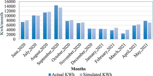
Figure 6. Average energy consumption per day.

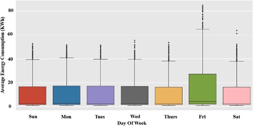
Figure 6 depicts the average hourly modelled energy use per day over the period of nearly a year. As can be observed, the building's energy usage is stable, with an hourly average of 15 kWh, except on Fridays, when the operational schedule is changed. On Fridays, the building is frequently used to its full capacity, causing the energy consumption to nearly double. The operational schedule for this facility was based on the official prayers timetable for the corresponding location.

3.2. Faults

Mosques, in general, are mainly furnished with HVAC units, lighting and other supplementary systems, such as sound systems and exhaust fans. In this research, the simulated faults primarily occur in the HVAC system, lighting control, and exhaust fans. The air conditioning system has four fault classes: thermostat offset (TO), dirty filter (DF), refrigerant undercharge (RU), and condenser fouling (CF). In contrast, the lighting and exhaust fans have a single fault each: occupancy sensor time delay (LCD) and exhaust fan-motor-worn-out (EXF). The faults were modelled using the EnergyPlus software, and their severities and the simulation parameters such as decrease in the cooling capacity, and fan pressure drops were added by utilizing a combination of information obtained from previous studies within the literature either through experimental records or simulation tools with comparable circumstances including dirty filter (Nassif 2012), condenser fouling (Qureshi and Zubair 2014), refrigerant undercharge (Fernandez et al. 2017), thermostat offset, lighting faults and fan motor degradation (Kim et al. 2019) as well as real-life maintenance work order histories from mosques with similar configurations within other regions of the kingdom of Saudi Arabia. Table 5 and Figure 7 list the simulated faults as well as their simulated severities. It is worth noting that the severity ranking of each fault (high, medium, and low) was determined based on the available simulated parameters as well as the impact ranks indicated on the maintenance work order records from the maintenance teams of the other mosques that were consulted. There were five levels of severity, with the first two being regarded as low, while the fourth and fifth were considered high. The third level was medium. Nevertheless, the refrigerant undercharge has only three severity levels based on the record within (Fernandez et al. 2017); thus, each severity represented one rank.

Figure 7. The simulated faults classes with different severities.

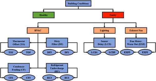
Table 5. Building’s simulated faults.

Systems	Faults	Introduced severity	Severity	Ranking
HVAC	Thermostat offset (TO)	TO1: ΔT =  + 1 °C	ΔT ≤ 2°C	Low
		TO2: ΔT =  + 2 °C
		TO3: ΔT =  + 3 °C	2°C < ΔT ≤ 3°C	Medium
		TO4: ΔT =  + 4 °C	ΔT > 3 °C	High
		TO5: ΔT =  + 5 °C
	Refrigerant undercharge (RU)	RU1: Leakage = 10%	Leakage ≤ 10%	Low
		RU2: Leakage = 20%	10% < Leakage ≤ 20%	Medium
		RU3: Leakage = 30%	Leakage > 20%	High
	Dirty filter (DF)	DF1: ΔP =  + 50%	ΔP ≤ 60%	Low
		DF2: ΔP =  + 60%
		DF3: ΔP =  + 70%	60% < ΔP ≤ 70%	Medium
		DF4: ΔP =  + 80%	ΔP > 70%	High
		DF5: ΔP =  + 90%
	Condenser fouling (CF)	CF1: Blockage = 50%	Blockage ≤ 60%	Low
		CF2: Blockage = 60%
		CF3: Blockage = 70%	60% < Blockage ≤ 70%	Medium
		CF4: Blockage = 80%	Blockage > 70%	High
		CF5: Blockage = 90%
Exhaust Fan	Exhaust Fan-Motor-Worn-Out (EXF)	EXF1: Fan Efficiency = −4%	−4% ≥ Efficiency drop ≤ −8%	Low
		EXF2: Fan Efficiency = −8%
		EXF3: Fan Efficiency = −12%	−8% < Efficiency drop ≤ −16%	Medium
		EXF4: Fan Efficiency = −16%	Efficiency drop > −16%	High
		EXF5: Fan Efficiency = −20%
Lighting Control	Occupancy sensor time delay (LCD)	LCD1: Sensor delay = 20 min	20 min ≥ Delay ≤ 30 min	Low
		LCD2: Sensor delay = 30 min
		LCD3: Sensor delay = 40 min	30 min < Delay ≤ 40 min	Medium
		LCD4: Sensor delay = 50 min	Delay > 40min	High
		LCD5: Sensor delay = 60 min

3.2. Data description

The FDD approaches in this research were trained and tested on weather and energy consumption data. The weather data utilized were achieved using an hourly sampling rate from the meteorological station at King Abdulaziz Airport. Date and time, day of the week, dry bulb temperature, dew point temperature, relative humidity, pressure, wind speed, and diffuse and direct solar radiation were all included in the data. The EnergyPlus simulation generated patterns of energy consumption under healthy and faulty conditions at an hourly sampling rate. Moreover, additional statistical features were derived from the modelled energy usage data, which included the mean, summation (sum) and standard deviation (std), and these were utilized as new aggregated features in relation to the day of the week. The fault impact rate, which is represented by Equation (6(6) $\begin{array}{rl}& \text{Fault Impact}\\ & =\frac{\begin{array}{c}\text{Energy Consumption}{}_{\text{Faulty}}\\ -\text{Energy Consumption}{}_{\text{Healthy}}\end{array}}{\text{Energy Consumption}{}_{\text{Healthy}}}\end{array}$(6) ), was also added as an additional feature which shows the hourly rise in energy consumption caused by the faults relative to a healthy condition. (6) $\begin{array}{rl}& \text{Fault Impact}\\ & =\frac{\begin{array}{c}\text{Energy Consumption}{}_{\text{Faulty}}\\ -\text{Energy Consumption}{}_{\text{Healthy}}\end{array}}{\text{Energy Consumption}{}_{\text{Healthy}}}\end{array}$(6) Some of the limitations of utilizing the energy consumption data in machine learning approaches may be solved by employing classical time series decomposition to obtain more detailed operational features of buildings. Time series decomposition techniques have been employed in a range of applications in the building sector, including energy forecasting (Zhu et al. 2021) and anomaly detection (Miller and Meggers 2017), but their applicability to fault diagnosis approaches has been limited. Thus, in the current study, the seasonal decomposition components of the modelled energy consumption were also employed as new features. The statistical seasonal decomposition tool is used to decompose time series into different components using a naive decomposition approach which is considered to be the classical decomposition approach. Moving averages are employed in classical decomposition to explore trend cycles and ‘seasonal’ or periodic behaviour. The trend cycles (T) depict the long-term nature of the data, whereas seasonal components (S) are indicated by the data’s periodic (i.e. daily) variation. Unexplained occurrences and uncertainty must also be evaluated to fully portray the nature of the data as represented by residual (R). The decomposition is mathematically represented as (Pickering et al. 2018): (7) ${\text{Y}}_{\text{t}}=\text{ f}({\text{T}}_{\text{t }},{\text{S}}_{\text{t }},{\text{R}}_{\text{t}})$(7) where; ${\text{Y}}_{\text{t}}$ is the original time series, ${\text{T}}_{\text{t }}$ is the trend component, ${\text{S}}_{\text{t }}$is the seasonal component, and ${\text{R}}_{\text{t}}$ the residual component.

The results were achieved by first identifying the trend in the data using a convolution filter with a linear filter (centred moving weighted average). The trend was then eliminated from the dataset, and the average of this de-trended series for each period was used to determine the seasonal component that was returned. In this study, a multiplicative model was applied since the building had daily and weekly seasonality patterns which reflected the nonlinearity of the building behaviour throughout the year. The multiplicative model implies that the components (trend, seasonal residual) are multiplied together as expressed in Equation (8(8) ${\text{Y}}_{\text{t}}={\text{T}}_{\text{t }}\times {\text{S}}_{\text{t }}\times {\text{R}}_{\text{t }}$(8) ), thus the original data is divided by the trend to obtain the detrended series (‘statsmodels.tsa.seasonal.seasonal_decompose — statsmodels’ 2022): (8) ${\text{Y}}_{\text{t}}={\text{T}}_{\text{t }}\times {\text{S}}_{\text{t }}\times {\text{R}}_{\text{t }}$(8) The proposed models were evaluated in this study using validation folds and an unseen testing set. The overall data size was an hourly dataset for a period of one year. The unseen dataset's portion was 10%, while the remaining 90% was used for the cross-validation part, including model training and validation. Since the dataset contained many features with various scales, the datasets were standardized and scaled using the standard scaler technique.

3.3. Classification evaluation

The evaluation stage is essential in determining the most appropriate classification techniques for the diagnostic process. The classification report includes various classification assessment parameters, including precision, recall, f-score, and accuracy. The classification report assessment gives either the classification performance of each class individually or the overall average classification accuracy of the entire model. The equations below depict each assessment metric in the classification report (Yan et al. 2020). (9) $\begin{array}{rl}\text{Precision}& =\frac{\text{TP}}{\text{TP}+\text{FP}}\end{array}$(9) (10) $\begin{array}{rl}\text{Recall}& =\frac{\text{TP}}{\text{TP}+\text{FN}}\end{array}$(10) (11) $\begin{array}{rl}\text{F}-\text{score}& =2\times \frac{\text{Precision}\times \text{Recall}}{\text{Precision}+\text{Recall}}\end{array}$(11) (12) $\begin{array}{rl}\text{Accuracy }& =\frac{\text{TP}+\text{TN}}{\text{TP}+\text{TN}+\text{FN}+\text{FP}}\end{array}$(12) where TP stands for true positives (the value represents the number of correctly categorized samples and corresponds to the current class). TN stands for true negatives (the value represents the number of correctly categorized samples and corresponds to the other class). FP stands for false positive (the value represents the number of incorrectly categorized samples and relates to the other classifications). And FN stands for false negative (The value represents the number of samples that were incorrectly categorized and relates to the current class). The classification accuracy in the current study indicates the total model classification accuracy across all the scenarios investigated. Meanwhile, the f-score was calculated to illustrate how successfully the model detected each faulty scenario individually. The training data was divided into several folds, as shown in Figure 8, using a cross-validation technique (Huang et al. 2022) to see how well the model worked on separate data segments and to refine the model parameters. Therefore, the overall model classification accuracy is the average of the accuracy of all the folds.

Figure 8. A schematic illustration of k-fold cross-validation on a dataset.

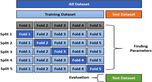
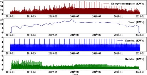
Figure 9. Time series decomposition components of one-year hourly energy consumption.

4. Result and discussion

The classical time series decomposition was performed on hourly modelled energy consumption for a period of one year. This enables the capture of seasonal and periodic periods throughout the day as a result of the nonlinear operating patterns caused by staggered and regularly changing prayer schedules. Figure 9 illustrates the entire decomposition components, including the original data, trend, seasonality, and residual. The original data (modelled data) demonstrates seasonality as a clear pattern that can be restored or recreated from these elements by combining the trend, seasonal, and residual components. The trend depicts the overall amplitude and evolution caused by the influence of weather-dependent operations related to the cooling system in the summer season. The trend component appears to shift significantly towards the summer months, albeit with fluctuation across the week interval. The seasonal component captures the daily and weekly energy consumption fluctuations throughout each day/week and repeats this exact seasonal component throughout the year. This reflects the daily and weekly seasonality based on the type of prayer and daily operational schedule. The seasonal component as can be seen in Figure 9 is evident at different times every day for the five prayers a day and has a strong spike every week owing to the weekly Friday prayer. This recurring seasonal component provides the most intriguing insights into a building's usual daily and weekly operations. Meanwhile, the residual component aggregates any deviations in the observed data from the trend and seasonal components. It mainly contains various irregular features because it includes events that are not explained by the daily and weekly periodicity, which are most probably unexpected interactions with the electric plug load or other non-HVAC equipment operations such as water coolers and fridges.

4.1. Features selection

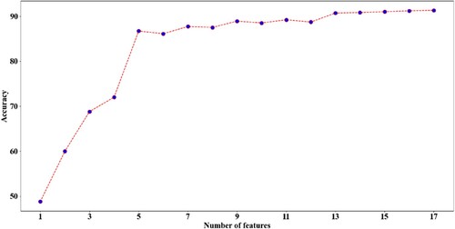
Certain features stood out more than others when it came to detecting investigated patterns. Feature selection strategies offer procedures for determining which features are most suited for class identification. In this study, the scikit-learn package's feature selection tools, particularly SelectKBest was applied, which is considered as a univariate filter tool that excludes everything except the K highest scoring features (specified by the user). The chosen rating score algorithm was f classif which computes the analysis of variance (ANOVA) F-value for the provided sample (Pedregosa et al. 2011). This is a common pattern for identifying the most important features in the dataset, and it is commonly used to reduce original data to a subset of features with the highest variation (Garali et al. 2016). Figure 10 depicts the importance score of the 17 training features. As can be observed, the fault impact, residual, and trend obtained the greatest scores in terms of energy usage. The fault impact obtained the best score since it reveals the increment rate created by the fault, allowing the classifier to easily identify the fault, assuming each fault has a distinct signature on the energy consumption. On the other hand, the seasonality element as well as the consumption statistical extracted elements (mean, summation, standard deviation) had a low importance score. Regarding meteorological data, the dew point temperature, relative humidity, and atmospheric pressure are more important. In terms of time-related elements, which may be due to weekly seasonality in the selected building, the number of days in the week is most important. To adjust the appropriate k value in the feature selection score, we compared the performance of the model using different k numbers (1–17). Therefore, the optimum classification performance was with all 17 features. As shown in Figure 11, an example of DT classification accuracy varies with the selection of the top k features. The best performance was achieved by utilizing most of the training features. Thus, in this study, all 17 features were employed to train the deployed classification models.

Figure 10. Importance of features in training data.

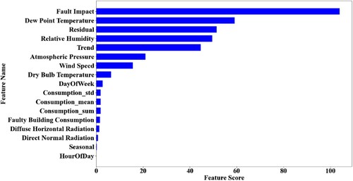
Figure 11. DT classification accuracy with the utilized number of features.

4.2. Algorithms’ fine-tuning

A critical step in enhancing classification accuracy and lowering the run time is fine-tuning the machine learning model. Thus, every model has its own set of parameters, and in this study, the models were tuned by adjusting the most important ones, such as the number of estimators in the RF and XGBoost, the kernel type in the SVC, and the activation function in the MLPC. Table 6 gives a list of the most significant tuning parameters for classification.

Table 6. Summary of main tuning parameters of each model.

Methods	Parameters	Values	Optimal
Features Number		[1,2, 3, … ..16,17]	17
LR	Regularization parameters ‘C’	[1,2,3,4 …  … .,99,100]	26
	LR Solver	[newton-cg, lbfgs, liblinear, sag, saga]	lbfgs
DT	Criterion	[gini, entropy, log_loss]	entropy
	Max_features	[auto,sqrt, log2, None]	None
RF	Criterion	[gini, entropy, log_loss]	entropy
	Estimators number	[100,250,500,750,1000,1250,1500,1750,2000]	1750
SVC	Kernel type	[Linear, poly, sigmoid, rbf]	rbf
	Regularization parameters ‘C’	[1,2,3,4 …  … .,99,100]	98
	gamma	[scale, auto]	scale
	Decision function shape	[ovo, ovr]	ovo
MLPC	Activation function	[ Identity, logistic, tanh, relu]	relu
	Solver	[lbfgs, sgd, adam]	adam
	Hidden layers number	[1,2,3,4,5]	5
GBC	Loss function	[log_loss, deviance, exponential]	deviance
	Estimators number	[100,250,500,750,1000,1250,1500,1750,2000]	1750
	Criterion	[friedman_mse,squared_error, mse]	mse
	Max_features	[auto, sqrt, log2, None]	None
XGBoost	Estimators number	[100,250,500,750,1000,1250,1500,1750,2000]	500
	Colsample_bytree	[0.1,0.2,0.3 …  … .0.8,.09,1.0]	0.3
	Max_depth	[1,2, 3, … ..,13,14,15]	15

4.3. Fault detection and diagnosis process

This study has two main sequential steps. The first is to classify the fault according to its type. The second is to classify the severity of each fault into distinct classes (low, medium or high). Therefore, the overall evaluation process is based on both investigation levels and validation with five folds cross-validation, as well as previously unseen testing data, to ensure robustness and generalisability of the proposed models.

Figure 12. The performance of classification models in classifying each fault type in the validation dataset.

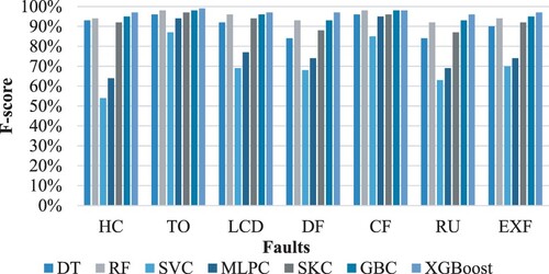
Figure 13. The performance of classification models in classifying each fault type in an unseen dataset.

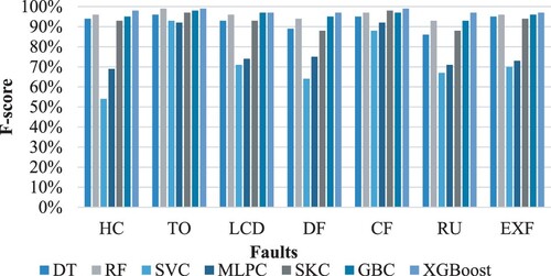
Figure 12 and Figure 13 show a comparison of f-score outcomes of the diagnosis of each fault type on both the validation and testing folds. As can be observed, ensemble techniques outperform conventional classifiers (DT, SVC, MLPC) in terms of classification performance. The tree-based classifier, whose base learner is the DT, outperformed the MLPC and SVC classifiers. Furthermore, the good performance of the one-layer ensemble stacking classifier was despite it consisting of conventional learner (DT, SVC, MLPC) and LR as the meta-classifier. However, this performance was achieved through the integration of DT. The HVAC system fault DF and RU were correctly diagnosed though slightly less accurately than other faults, particularly by DT, SKC, RF, and GBC. The diagnostic score of the TO fault, on the other hand, was the best for most of the classifiers. This variation in the diagnosis score may be because the model was trained with varying fault severities and that distinct faults may have the same symptoms and faulty conditions which led to an increase in the fault misdiagnosis rate. In terms of model generalization, all of the proposed models performed identically with regards to validation effectiveness. There was an average of about 1% improvement in the testing process in most models, indicating that the training process was generalized and the models were trained on the majority of investigated scenarios. This implies that the training sample effectively covered all of the cases observed in the domain. Furthermore, shuffling the dataset ensured that the same algorithm was performed on new data each time to cover distinct patterns of random features and repeating the model assessment process using cross-validation to govern the randomness on training the model. As mentioned earlier, this study has two levels of investigation: fault type and fault severity classification. Since the fault severity classification was trained by utilizing the first level's output prediction, the classification accuracy was highly dependent on the former.

Figure 14. The performance of classification models in classifying the fault type and severity in the validation dataset.

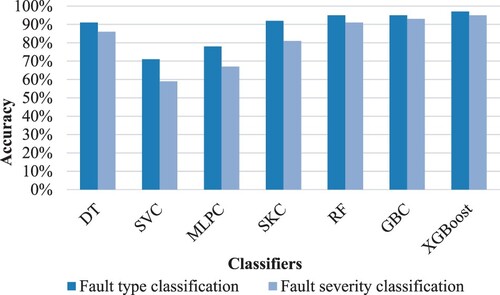
Figure 15. The performance of classification models in classifying the fault type and severity in an unseen dataset.

Figure 14 and Figure 15 compare the overall classification accuracy of the proposed models in classifying the fault type and severity in the validation and the unseen datasets. Overall, the accuracies of the fault severity classification were slightly lower than the fault type identification accuracy. The SVM and MLPC had the worst classification accuracy for both levels, especially in terms of the severity range classification, which performed with about 59% and 67%, respectively, in validation folds and about 56% and 71% in the testing data set. The ensemble classifier (RF, GBC and XGBoost) recognized the faults and classified their severity with very high accuracy, more than other classifiers, with a minimum gap between the accuracy of the two levels. The XGBoost had about 97% and 95% accuracy on both levels on the validation portion and about 98% and 96% on the testing folds. Although the SKC had a good accuracy on fault type identification (roughly 92%), its performance dropped by almost 11% in severity classification. This is due to a notable performance discrepancy between the two levels resulting from its base learners (DT, SVC, MLPC), which were around 5%, 17%, and 14%, respectively. The XGBoost outperformed all other classifiers for both levels and dataset segments, followed by the GBC and RF.

Decomposition is a principle that can be employed to comprehend complexities during time series analysis and to assist models in capturing irregular building behaviour. The outstanding diagnostic accuracy might not be achieved while using building energy consumption as raw data in the learning phase, considering that building operations are not linear processes. Therefore, the time series decomposition components (T, S, R) of the modelled energy consumption reading were included as training features to prove their enhancement of the classification approaches. Table 7 illustrates a comparison of the overall classification accuracy in validation folds concerning the inclusion of the time series decomposition component in the diagnosis process. As seen in the table below, the classification accuracy with decomposition is significantly better at both analysis levels than without the components. Furthermore, the improvement rate of the decomposition components in the fault severity classification accuracy was substantially higher than the fault type classification, improving the classifier's accuracy by 33% on average. Meanwhile, the top three best ensemble techniques on the faults identification level (RF, GBC, and XGBoost) had the lowest enhancement rate of roughly 9%. This table shows how significant the time series decomposition components are in FDD approaches for learning and accuracy enhancement.

Table 7. A comparison of the model’s accuracy in relation to the utilization of data decomposition components.

	Fault type classification
	DT	SVC	MLPC	SKC	RF	GBC	XGBoost
Without Decomposition	80%	59%	66%	83%	87%	87%	89%
With Decomposition	91%	71%	78%	92%	95%	95%	97%
	Fault severity classification
Without Decomposition	60%	44%	49%	60%	72%	71%	75%
With Decomposition	86%	59%	67%	81%	91%	93%	95%

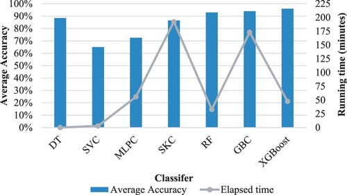
Figure 16. A comparison of average classification accuracy with the runtime in minutes.

4.4. Models running time

Although diagnostic accuracy is essential for adopting FDD techniques, other parameters, such as computational efficacy, are also significant because they affect downtime periods, which are significantly associated with overall operational cost. As a result, the elapsed time for the overall diagnosis process was determined for each classification model using Python's time package (Padmanabhan 2016). Figure 16 depicts a comparison of average classification accuracy between the two levels of analysis in the validation dataset with the runtime in minutes. As can be seen, a considerable variation in running time between the classifiers was employed. With regard to the conventional algorithms, MLPC required the longest processing time (about 56 min), whereas the timeframes required by the other classifiers (DT and SVC) were around 0.1 and 3 min, respectively. Similarly, there was a significant difference in the running duration of the ensemble technique. The RF and XGBoost took less time (about 33 and 47 min respectively) than the GBC and SKC, which required around 173 and 192 min, respectively. With regard to the average classification accuracy, the top three classifiers that were rated with an average accuracy above 90% were RF, GBC and XGBoost, with 93.0%, 94.0% and 96.0%, respectively. The graph shows how optimization on the XGBoost classifier made it faster than traditional boosting in terms of running time. This helped to reduce the running time by about 72%. To expand the selection criteria based on the accuracy and computational time, the XGBoost can be considered to be the best diagnostic classifier, in this case, despite the slight superiority of the RF in terms of run time.

4.5. The effect of adding noise to the training dataset

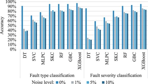
Noise was added to the modelled data to mimic the influence of random processes that occur in nature to investigate the robustness of the proposed models under noisy conditions. The current research adopted a Gaussian distribution with a zero mean and a standard deviation, and the level of noise introduced into the dataset is controlled by the value of standard deviation (Adams et al. 2019). The noise levels were determined based on prior research within the literature and determined to be 1%, 5%, and 10% of the standard deviation in the modelled energy usage (Fan et al. 2022). As shown in Figure 17, incorporating noise has a significant impact on model performance. As the noise level increases, classification performance degrades by up to 66%. However, this influence fluctuates, indicating that there is a difference in model performance in terms of noise sensitivity. The performance of DT, for example, declined from around 91% to approximately 40% on fault type classification and from 86% to approximately 22% on the severity classification phase. The XGBoost, on the other hand, had a much lesser effect, decreasing classification accuracy from 97% to about 87% on average in the fault type classification and from 95% to around 84% in the severity classification.

Figure 17. Classification accuracy of the proposed models under different noise levels.

This study shows that the inclusion of time series decomposition components generally led to an enhancement of classification accuracy, particularly when classifying fault severity. The extensive comparisons undertaken in this work are expected to boost researchers’ confidence in choosing the most appropriate classification approaches. As a result, the ensemble classifiers showed excellent classification accuracy compared with conventional ones; however, the running time concern led to the exclusion of most of them in the current study. The XGBoost classifier obtained the highest classification accuracy during the validation and testing stages even with the addition of varying levels of noise. The classification of the fault's corresponding severity will let the building owners and occupants realize proper maintenance decisions and the seriousness of the fault's impact on building performance.

5. Conclusion

Ensemble-based FDD techniques were utilized to analyse faults that affect patterns of energy consumption of buildings. The EnergyPlus software was used to replicate the target building and the investigated faults. The introduced faults included several building systems, such as HVAC, lighting, and exhaust fans, with varying degrees of severity, to identify both the fault type and the severity range. The weather data, modelled energy usage, and statistical extracted features were combined to train the classification models. The model assessment was conducted on cross-validation and an unseen dataset to evaluate the model performance generalization. Ensemble-based classification approaches, including RF, SKC, GBC and XGBoost, were applied to identify the root causes of the anomalous behaviour and the severity rating. To adequately support their selection, the classification evaluation metrics of various ensemble approaches for building-level failure diagnostics were assessed for both analyses (fault type and severity rating). The classification accuracy with the inclusion of the statistical decomposition components was much higher than without them in both analyses. Furthermore, the fault severity classification accuracy improved at a better rate than the fault type classification. The XGBoost identified the faults and classified their severities with better accuracy than other classifiers, with a narrower gap between the accuracies of the two analyses with an average accuracy of 96% and with a reasonable running time of about 47 min. Moreover, the diagnostic ability of the proposed models decreased when noise was added to the training dataset, but XGBoost still performed well in terms of noise sensitivity when compared to other classifiers. Testing the capabilities of the ensemble classification approach indicated that they had a promising performance among other classifiers, while some still had high running times, such as GBC and SKC, which may be addressed by using RF and XGBoost. Finally, it would be advantageous to assess the performance of XGBoost on various building types, systems and climatic regions to better validate its adaptability. In addition, despite the promised performance of the classical decomposition method in enhancing the classification accuracy, other advanced approaches can be used in future work such as trend decomposition using loess (STL).

Disclosure statement

No potential conflict of interest was reported by the author(s).

Data availability statement

The data that support the findings of this study are available from the corresponding author, [AYK], upon reasonable request.

Appendices

Appendix A

Table

List of Abbreviations
A/C	Air conditioning
AdaBoost	Adaptive boosting
AHU	Air handling unit
ANN	Artificial neural network
BEMS	Building energy management systems
CBM	Condition-based maintenance
CF	Condenser fouling
CO2	Carbon dioxide
DF	Dirty filter
DX	Direct expansion
DNN	Deep neural network
DT	Decision tree
EDM	Ensemble diagnostic model
EU	European Union
EXF	Exhaust fan-motor-worn-out
FFD	Fault detection and diagnosis
FN	False negative
FP	False positive
GBC	Gradient boosting classifier
HC	Healthy condition
HVAC	Heating ventilation air conditioning
KNN	k-nearest neighbours
KSA	Kingdom of Saudi Arabia
LCD	Occupancy sensor time delay
LightGBM	Light gradient boosting machine
LR	Logistic regression
LSTM	Long short-term memory
MLPC	Multi-layer perceptron classifier
PIAs	Physical industrial assets
PPM	Planned preventive maintenance
PTAC	Packaged terminal air conditioner
R	Residual
RF	Random forest
RM	Reactive maintenance
RU	Refrigerant undercharge
S	Seasonal components
SKC	Stacking classifier
SNN	Shallow neural networks
Std	The standard deviation
Sum	The summation
SVC	Support vector classifier
SVM	Support vector machines
T	Trend cycles
TN	True negatives
TO	Thermostat offset
TP	True positives
TRNSYS	Transient system simulation tool
UK	United Kingdom
VAV	Variable-air-volume
XGBoost	Extreme gradient boosting

Appendix B

Table

List of Nomenclature
$\mathrm{\varnothing }(\mathbf{\text{x}}{)}_{\mathbf{\text{i}}}$	Non-linear transformation that converts input data to a high-dimensional feature space in SVC
C	The cost parameter that denotes the trade-off between computational complexity and training error in SVC
${\mathit{P}}_{\mathit{j}}({\mathit{x}}_{\mathit{i}})$	Probability of fault class j in LR
T	The number of leaves in a decision tree in XGBoost
w	Weight vector in SVC
${\mathit{y}}_{\mathit{i}}$	Actual value XGBoost
$\widehat{{\mathit{y}}_{\mathit{i}}}$	Prediction value XGBoost
α	The intercept in LR
β	The coefficients that are linked to the explanatory variable in LR
$\mathit{\gamma }$	Leaf's complexity XGBoost
λ	Scaling parameter for the penalty's severity XGBoost
ξ	The slack variable to deal with misclassification in SVC
$\mathbf{\Omega }(\mathbf{\text{f}})$	Regularization that penalizes the model's complexity of XGBoost

References

- Adams, S., S. Greenspan, M. Velez-Rojas, S. Mankovski, and P. A. Beling. 2019. “Data-driven Simulation for Energy Consumption Estimation in a Smart Home.” Environment Systems and Decisions 39 (3): 281–294. https://doi.org/10.1007/s10669-019-09727-1.
- Ahn, B. C., J. W. Mitchell, and I. B. D. McIntosh. 2001. “Model-Based Fault Detection and Diagnosis for Cooling Towers.” ASHRAE Transactions 107: 967–974.
- Alexandersen, E. K., M. R. Skydt, S. S. Engelsgaard, M. Bang, M. Jradi, and H. R. Shaker. 2019. “A Stair-Step Probabilistic Approach for Automatic Anomaly Detection in Building Ventilation System Operation.” Building and Environment 157: 165–171. https://doi.org/10.1016/j.buildenv.2019.04.036.
- Alghanmi, A., A. Yunusa-Kaltungo, and R. Edwards. 2021. “A Comparative Study of Faults Detection Techniques on HVAC Systems.” https://doi.org/10.1109/PowerAfrica52236.2021.9543158.
- Alghanmi, A., A. Yunusa-kaltungo, and R. E. Edwards. 2022. “Investigating the Influence of Maintenance Strategies on Building Energy Performance: A Systematic Literature Review.” Energy Reports 8: 14673–14698. https://doi.org/10.1016/j.egyr.2022.10.441.
- Andriamamonjy, A., D. Saelens, and R. Klein. 2018. “An Auto-Deployed Model-Based Fault Detection and Diagnosis Approach for Air Handling Units Using BIM and Modelica.” Automation in Construction 96: 508–526. https://doi.org/10.1016/j.autcon.2018.09.016.
- Atkinson, P. M., and A. R. L. Tatnall. 1997. “Introduction Neural Networks in Remote Sensing.” International Journal of Remote Sensing 18 (4): 699–709. https://doi.org/10.1080/014311697218700.
- Ayu, K., and A. Yunusa-Kaltungo. 2020. “A Holistic Framework for Supporting Maintenance and Asset Management Life Cycle Decisions for Power Systems.” Energies 13 (8), https://doi.org/10.3390/en13081937.
- Azadeh, A., M. Saberi, A. Kazem, V. Ebrahimipour, A. Nourmohammadzadeh, and Z. Saberi. 2013. “A Flexible Algorithm for Fault Diagnosis in a Centrifugal Pump with Corrupted Data and Noise Based on ANN and Support Vector Machine with Hyper-Parameters Optimization.” Applied Soft Computing Journal 13 (3): 1478–1485. https://doi.org/10.1016/j.asoc.2012.06.020.
- Benkercha, R., and S. Moulahoum. 2018. “Fault Detection and Diagnosis Based on C4.5 Decision Tree Algorithm for Grid Connected PV System.” Solar Energy 173: 610–634. https://doi.org/10.1016/j.solener.2018.07.089.
- Bin Yang, X., X. Q. Jin, Z. M. Du, B. Fan, and Y. H. Zhu. 2014. “Optimum Operating Performance Based Online Fault-Tolerant Control Strategy for Sensor Faults in air Conditioning Systems.” Automation in Construction 37: 145–154. https://doi.org/10.1016/j.autcon.2013.10.011.
- Chakraborty, D., and H. Elzarka. 2019. “Early Detection of Faults in HVAC Systems Using an XGBoost Model with a Dynamic Threshold.” Energy and Buildings 185: 326–344. https://doi.org/10.1016/j.enbuild.2018.12.032.
- Chen, Z., F. Han, L. Wu, J. Yu, S. Cheng, P. Lin, and H. Chen. 2018. “Random Forest Based Intelligent Fault Diagnosis for PV Arrays Using Array Voltage and String Currents.” Energy Conversion and Management 178: 250–264. https://doi.org/10.1016/j.enconman.2018.10.040.
- Chen, Y., and J. Wen. 2018. “Development and Field Evaluation of Data-Driven Whole Building Fault Detection and Diagnosis Strategy.” In Proceedings of the Annual Conference of the Prognostics and Health Management Society, PHM, 1–8. https://doi.org/10.36001/phmconf.2018.v10i1.517.
- D. and G. Ministry of Islamic Affairs. 2021. “Statistical book for the fiscal year 1440/1441 AH,” Dar Al Watan for Publishing, 2021. [Online]. https://www.moia.gov.sa/Statistics/Pages/Details.aspx?ID=10.
- Del Frate, F., F. Pacifici, G. Schiavon, and C. Solimini. 2007. “Use of Neural Networks for Automatic Classification from High-Resolution Images.” IEEE Transactions on Geoscience and Remote Sensing 45 (4): 800–809. https://doi.org/10.1109/TGRS.2007.892009.
- Ebrahimifakhar, A., A. Kabirikopaei, and D. Yuill. 2020. “Data-driven Fault Detection and Diagnosis for Packaged Rooftop Units Using Statistical Machine Learning Classification Methods.” Energy and Buildings 225. https://doi.org/10.1016/j.enbuild.2020.110318.
- European Parliament. 2019. “Reducing Carbon Emissions: Eu targets and Measures.” News European Parliament. Accessed September 08, 2022. https://www.europarl.europa.eu/pdfs/news/expert/2018/3/story/20180305STO99003/20180305STO99003_en.pdf.
- Fan, C., M. Chen, R. Tang, and J. Wang. 2022. “A Novel Deep Generative Modeling-Based Data Augmentation Strategy for Improving Short-Term Building Energy Predictions.” Building Simulation 15 (2): 197–211. https://doi.org/10.1007/s12273-021-0807-6.
- Fan, C., Y. Liu, X. Liu, Y. Sun, and J. Wang. 2021. “A Study on Semi-Supervised Learning in Enhancing Performance of AHU Unseen Fault Detection with Limited Labeled Data.” Sustainable Cities and Society 70. https://doi.org/10.1016/j.scs.2021.102874.
- Fernandez, N., Y. Xie, S. Katipamula, M. Zhao, W. Wang, and C. Corbin. 2017. “Impacts of Commercial Building Controls on Energy Savings and Peak Load Reduction,” Washington.
- Gao, D. C., S. Wang, W. Gang, and F. Xiao. 2016. “A Model-Based Adaptive Method for Evaluating the Energy Impact of low Delta-T Syndrome in Complex HVAC Systems Using Support Vector Regression.” Building Services Engineering Research and Technology 37 (5): 576–596. https://doi.org/10.1177/0143624416640760.
- Garali, I., M. Adel, S. Bourennane, M. Ceccaldi, and E. Guedj. 2016. “Brain Region of Interest Selection for 18FDG Positrons Emission Tomography Computer-Aided Image Classification.” Irbm 37 (1): 23–30. https://doi.org/10.1016/j.irbm.2015.10.002.
- Gunay, B., W. Shen, B. Huchuk, C. Yang, S. Bucking, and W. O’Brien. 2018. “Energy and Comfort Performance Benefits of Early Detection of Building Sensor and Actuator Faults.” Building Services Engineering Research and Technology 39 (6): 652–666. https://doi.org/10.1177/0143624418769264.
- Guo, Y., J. Wang, H. Chen, G. Li, R. Huang, Y. Yuan, T. Ahmad, and S. Sun. 2019. “An Expert Rule-Based Fault Diagnosis Strategy for Variable Refrigerant Flow air Conditioning Systems.” Applied Thermal Engineering 149: 1223–1235. https://doi.org/10.1016/j.applthermaleng.2018.12.132.
- Han, H., Z. Zhang, X. Cui, and Q. Meng. 2020. “Ensemble Learning with Member Optimization for Fault Diagnosis of a Building Energy System.” Energy Build. (Netherlands) 226: 97–110. [Online]. http://doi.org/10.1016/j.enbuild.2020.110351.
- Huang, J., J. Wen, H. Yoon, O. Pradhan, T. Wu, Z. O’Neill, and K. Selcuk Candan. 2022. “Real vs. Simulated: Questions on the Capability of Simulated Datasets on Building Fault Detection for Energy Efficiency from a Data-Driven Perspective.” Energy and Buildings 259. https://doi.org/10.1016/j.enbuild.2022.111872.
- International Energy Agency. 2022. “Buildings: A Source of Enormous Untapped Efficiency Potential.” nternational Energy Agency. Accessed September 08, 2022. https://www.iea.org/topics/buildings.
- Kang, S., S. Cho, and P. Kang. 2015. “Multi-class Classification via Heterogeneous Ensemble of one-Class Classifiers.” Engineering Applications of Artificial Intelligence 43: 35–43. https://doi.org/10.1016/j.engappai.2015.04.003.
- Kang, H., and S. Kang. 2021. “A Stacking Ensemble Classifier with Handcrafted and Convolutional Features for Wafer map Pattern Classification.” Computers in Industry 129. https://doi.org/10.1016/j.compind.2021.103450.
- Kim, J., S. Frank, J. E. Braun, and D. Goldwasser. 2019. “Representing Small Commercial Building Faults in EnergyPlus, Part I: Model Development.” Buildings 9 (11). https://doi.org/10.3390/buildings9110233.
- Krawczyk, B., L. L. Minku, J. Gama, J. Stefanowski, and M. Woźniak. 2017. “Ensemble Learning for Data Stream Analysis: A Survey.” Information Fusion 37: 132–156. https://doi.org/10.1016/j.inffus.2017.02.004.
- Kumar, A., and M. Jain. 2020. Ensemble Learning for AI Developers. Berkeley, CA: Apress.
- Li, G., Y. Hu, J. Liu, X. Fang, and J. Kang. 2021. “Review on Fault Detection and Diagnosis Feature Engineering in Building Heating, Ventilation, Air Conditioning and Refrigeration Systems.” IEEE Access (USA) 9: 2153–2187. [Online]. https://doi.org/10.1109/ACCESS.2020.3040980
- Lin, G., and D. E. Claridge. 2015. “A Temperature-Based Approach to Detect Abnormal Building Energy Consumption.” Energy and Buildings 93: 110–118. https://doi.org/10.1016/j.enbuild.2015.02.013.
- Luwei, K. C., A. Yunusa-Kaltungo, and Y. A. Sha’aban. 2018. “Integrated Fault Detection Framework for Classifying Rotating Machine Faults Using Frequency Domain Data Fusion and Artificial Neural Networks.” Machines 6 (4): 59. https://doi.org/10.3390/MACHINES6040059.
- Mavromatidis, G., S. Acha, and N. Shah. 2013. “Diagnostic Tools of Energy Performance for Supermarkets Using Artificial Neural Network Algorithms.” Energy and Buildings 62: 304–314. https://doi.org/10.1016/j.enbuild.2013.03.020.
- McHugh, M. K., T. Isakson, and Z. Nagy. 2019. “Data-driven Leakage Detection in air-Handling Units on a University Campus.” ASHRAE Transactions 125: 381–388.
- Menahem, E., L. Rokach, and Y. Elovici. 2009. “Troika - An Improved Stacking Schema for Classification Tasks.” Information Sciences 179 (24): 4097–4122. https://doi.org/10.1016/j.ins.2009.08.025.
- Miller, C., and F. Meggers. 2017. “Mining Electrical Meter Data to Predict Principal Building use, Performance Class, and Operations Strategy for Hundreds of non-Residential Buildings.” Energy and Buildings 156: 360–373. https://doi.org/10.1016/j.enbuild.2017.09.056.
- Mishra, K. M., and K. Huhtala. 2019. “Elevator Fault Detection Using Profile Extraction and Deep Autoencoder Feature Extraction for Acceleration and Magnetic Signals.” Applied Sciences 9 (15): 2990. https://doi.org/10.3390/app9152990.
- Nassif, N. 2012. “The Impact of air Filter Pressure Drop on the Performance of Typical air-Conditioning Systems.” Building Simulation 5 (4): 345–350. https://doi.org/10.1007/s12273-012-0091-6.
- Padmanabhan, T. R. 2016. “Python–A Calculator.” In Programming with Python, edited by T. R. Padmanabhan, 1–5. Singapore: Springer. https://doi.org/10.1007/978-981-10-3277-6_1
- Pandya, D. H., S. H. Upadhyay, and S. P. Harsha. 2014. “Fault Diagnosis of Rolling Element Bearing by Using Multinomial Logistic Regression and Wavelet Packet Transform.” Soft Computing 18 (2): 255–266. https://doi.org/10.1007/s00500-013-1055-1.
- Patrick Schneider, F. X. 2022. “Machine Learning.” Anomaly Detection and Complex Event Processing Over IoT Data Streams 45 (13): 40–48.
- Pedregosa, F., G. Varoquaux, A. Gramfort, P. Michel, B. Thirion, O. Grisel, M. Blondel, P. Prettenhofer, R. Weiss, and V. Dubourg. 2011. “Scikit-learn: Machine Learning in {P}ython.” Journal of Machine Learning Research, 2825–2830. Accessed June 03, 2022. [Online]. https://scikit-learn.org/stable/modules/generated/sklearn.feature_selection.SelectKBest.html.
- Pickering, E. M., M. A. Hossain, R. H. French, and A. R. Abramson. 2018. “Building Electricity Consumption: Data Analytics of Building Operations with Classical Time Series Decomposition and Case Based Subsetting.” Energy and Buildings 177: 184–196. https://doi.org/10.1016/j.enbuild.2018.07.056.
- Piscitelli, M. S., S. Brandi, A. Capozzoli, and F. Xiao. 2021. “A Data Analytics-Based Tool for the Detection and Diagnosis of Anomalous Daily Energy Patterns in Buildings.” Building Simulation 14 (1). https://doi.org/10.1007/s12273-020-0650-1.
- Qiao, Q., A. Yunusa-Kaltungo, and R. E. Edwards. 2021. “Towards Developing a Systematic Knowledge Trend for Building Energy Consumption Prediction.” Journal of Building Engineering 35: 101967. https://doi.org/10.1016/j.jobe.2020.101967.
- Qureshi, B. A., and S. M. Zubair. 2014. “The Impact of Fouling on the Condenser of a Vapor Compression Refrigeration System: An Experimental Observation.” International Journal of Refrigeration 38 (1): 260–266. https://doi.org/10.1016/j.ijrefrig.2013.08.012.
- Schein, J., S. T. Bushby, N. S. Castro, and J. M. House. 2006. “A Rule-Based Fault Detection Method for air Handling Units.” Energy and Buildings 38 (12): 1485–1492. https://doi.org/10.1016/j.enbuild.2006.04.014.
- SGI. 2021. “His Royal Highness the Crown Prince announces the Kingdom of Saudi Arabia’s aims to achieve net zero emissions by 2060,” 2021. [Online]. https://www.saudigreeninitiative.org/pr/SGI_Forum_Press_Release-EN.pdf.
- Shohet, R., M. S. Kandil, and J. J. McArthur. 2019. “Machine Learning Algorithms for Classification of Boiler Faults Using a Simulated Dataset.” IOP Conference Series: Materials Science and Engineering 609 (6): 062007. (6 pp.), [Online]. https://doi.org/10.1088/1757-899X/609/6/062007
- Shohet, R., M. S. Kandil, Y. Wang, and J. J. McArthur. 2020. “Fault Detection for non-Condensing Boilers Using Simulated Building Automation System Sensor Data.” Advanced Engineering Informatics 46. [Online]. https://doi.org/10.1016/j.aei.2020.101176
- Singh, V., J. Mathur, and A. Bhatia. 2022. “A Comprehensive Review: Fault Detection, Diagnostics, Prognostics, and Fault Modeling in HVAC Systems.” International Journal of Refrigeration 144 (August): 283–295. https://doi.org/10.1016/j.ijrefrig.2022.08.017.
- Sopiyan, M., F. Fauziah, and Y. F. Wijaya. 2022. “Fraud Detection Using Random Forest Classifier, Logistic Regression, and Gradient Boosting Classifier Algorithms on Credit Cards.” JUITA: Jurnal Informatika 10 (1): 77. https://doi.org/10.30595/juita.v10i1.12050.
- “statsmodels.tsa.seasonal.seasonal_decompose — statsmodels”. 2022. Accessed October 03, 2022. https://www.statsmodels.org/dev/generated/statsmodels.tsa.seasonal.seasonal_decompose.html.
- Sun, L., J. Wu, H. Jia, and X. Liu. 2017. “Research on Fault Detection Method for Heat Pump air Conditioning System Under Cold Weather.” Chinese Journal of Chemical Engineering 25 (12): 1812–1819. https://doi.org/10.1016/j.cjche.2017.06.009.
- Sutton, C. D. 2005. “Classification and Regression Trees, Bagging, and Boosting.” Handbook of Statistics 24: 303–29.
- Szczerbicki, E. 2001. “Management of Complexity and Information Flow.” In Agile Manufacturing: The 21st Century Competitive Strategy, 247–263. Elsevier Science Ltd.
- Toma, R. N., A. E. Prosvirin, and J. M. Kim. 2020. “Bearing Fault Diagnosis of Induction Motors Using a Genetic Algorithm and Machine Learning Classifiers.” Sensors 20 (7). https://doi.org/10.3390/s20071884.
- Tran, D. A. T., Y. Chen, and C. Jiang. 2016. “Comparative Investigations on Reference Models for Fault Detection and Diagnosis in Centrifugal Chiller Systems.” Energy and Buildings 133: 246–256. https://doi.org/10.1016/j.enbuild.2016.09.062.
- Trizoglou, P., X. Liu, and Z. Lin. 2021. “Fault Detection by an Ensemble Framework of Extreme Gradient Boosting (XGBoost) in the Operation of Offshore Wind Turbines.” Renewable Energy 179: 945–962. https://doi.org/10.1016/j.renene.2021.07.085.
- Wei, D., H. Feng, Q. Han, and K. Jia. 2022. “Fault Detection and Diagnosis for Variable-air-Volume Systems Using Combined Residual, Qualitative and Quantitative Techniques.” Energy and Buildings 254. https://doi.org/10.1016/j.enbuild.2021.111491.
- Yan, K., J. Huang, W. Shen, and Z. Ji. 2020. “Unsupervised Learning for Fault Detection and Diagnosis of air Handling Units.” Energy and Buildings 210: 109689. https://doi.org/10.1016/j.enbuild.2019.109689.
- Yan, J., and J. Lee. 2005. “Degradation Assessment and Fault Modes Classification Using Logistic Regression.” Journal of Manufacturing Science and Engineering 127 (4): 912–914. https://doi.org/10.1115/1.1962019.
- Yan, K., W. Shen, T. Mulumba, and A. Afshari. 2014. “ARX Model Based Fault Detection and Diagnosis for Chillers Using Support Vector Machines.” Energy and Buildings 81: 287–295. https://doi.org/10.1016/j.enbuild.2014.05.049.
- Yan, C., S. Wang, F. Xiao, and D. ce Gao. 2015. “A Multi-Level Energy Performance Diagnosis Method for Energy Information Poor Buildings.” Energy 83: 189–203. https://doi.org/10.1016/j.energy.2015.02.014.
- Yao, W., D. Li, and L. Gao. 2022. “Fault Detection and Diagnosis Using Tree-Based Ensemble Learning Methods and Multivariate Control Charts for Centrifugal Chillers.” Journal of Building Engineering 51. https://doi.org/10.1016/j.jobe.2022.104243.
- Yu, Y., D. Woradechjumroen, and D. Yu. 2014. “A Review of Fault Detection and Diagnosis Methodologies on air-Handling Units.” Energy and Buildings 82: 550–562. https://doi.org/10.1016/j.enbuild.2014.06.042.
- Yun, W.-S., W.-H. Hong, and H. Seo. 2021. “A Data-Driven Fault Detection and Diagnosis Scheme for air Handling Units in Building HVAC Systems Considering Undefined States.” Journal of Building Engineering 35. https://doi.org/10.1016/j.jobe.2020.102111.
- Yunusa-Kaltungo, A., M. M. Kermani, and A. Labib. 2017. “Investigation of Critical Failures Using Root Cause Analysis Methods: Case Study of ASH Cement PLC.” Engineering Failure Analysis 73: 25–45. https://doi.org/10.1016/j.engfailanal.2016.11.016.
- Yunusa-Kaltungo, A., and A. Labib. 2021. “A Hybrid of Industrial Maintenance Decision Making Grids.” Production Planning and Control 32 (5): 397–414. https://doi.org/10.1080/09537287.2020.1741046.
- Yunusa-Kaltungo, A., and J. K. Sinha. 2017. “Effective Vibration-Based Condition Monitoring (eVCM) of Rotating Machines.” Journal of Quality in Maintenance Engineering 23 (3): 279–296. https://doi.org/10.1108/JQME-08-2016-0036.
- Zhao, Y., T. Li, X. Zhang, and C. Zhang. 2019. “Artificial Intelligence-Based Fault Detection and Diagnosis Methods for Building Energy Systems: Advantages, Challenges and the Future.” Renewable and Sustainable Energy Reviews 109 (April): 85–101. https://doi.org/10.1016/j.rser.2019.04.021.
- Zhou, Z., G. Li, J. Wang, H. Chen, H. Zhong, and Z. Cao. 2020. “A Comparison Study of Basic Data-Driven Fault Diagnosis Methods for Variable Refrigerant Flow System.” Energy and Buildings 224: 119–132. https://doi.org/10.1016/j.enbuild.2020.110232.
- Zhu, X., Z. Du, X. Jin, and Z. Chen. 2019. “Fault Diagnosis Based Operation Risk Evaluation for air Conditioning Systems in Data Centers.” Building and Environment 163. [Online]. http://doi.org/10.1016/j.buildenv.2019.106319.
- Zhu, G., S. Peng, Y. Lao, Q. Su, and Q. Sun. 2021. “Short-Term Electricity Consumption Forecasting Based on the EMD-Fbprophet-LSTM Method.” Mathematical Problems in Engineering 2021. https://doi.org/10.1155/2021/6613604.