Risk of incorrect choices due to uncertainty in BPS evaluations of conceptual-stage neighbourhood-scale building designs

Abstract

At the conceptual-stage, building performance simulation (BPS) based evaluations are being increasingly used for tasks such as ranking of competing massing design proposals. However, such conceptual stage evaluations suffer from information deficiency in building level design attributes. The resulting uncertainty in performance evaluations raises questions regarding their usefulness for decision-making. We used a risk-based decision evaluation metric called expected opportunity loss to assess the reliability of a BPS-based ranking of conceptual stage massing schemes. We found daylighting assessments (spatial Daylight Autonomy) to be least reliable, with 22% chance of making an incorrect decision at the conceptual stage, followed by annual heating (15%) and cooling demand (8%). This work provides a structured framework for evaluating utility of conceptual stage BPS models and a purposeful basis for integration of BPS assessments in the design process, subject to level of design development.

KEYWORDS:

• Early design
• level of detail
• massing models
• BPS user
• design process
• robust decision-making

1. Introduction and state of the art

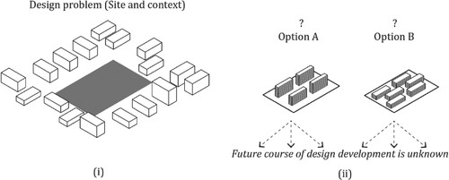
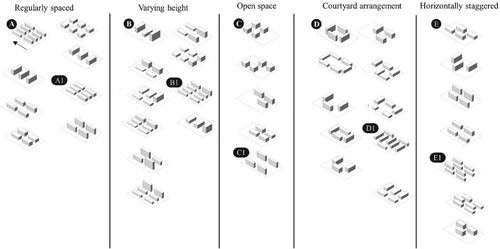
The building performance simulation community (e.g., ASHRAE 2018; CIBSE 2015), the architectural design community (e.g., AIA 2019) and city/state governments (e.g., BC Housing et al. 2018; SIA 2017) have all asserted the need for building performance assessments at multiple stages of the design process. The early design stage, i.e. when the built form or the shape of the building enclosures is being determined, is of particularly high interest to all parties mentioned above, as design choices made at this time can have a large effect on several comfort and energy-use related performance criteria (Compagnon 2004; Okeil 2010; Sattrup and Strømann-Andersen 2013). Design proposals at this stage are often represented as block models or massing-schemes: what we mean with massing-scheme in this context is the volumetric bounds of the built mass as per the design proposal made for a given site, exemplified for instance in Figure 1.

Figure 1. Common design decision problem where a design alternative needs to be chosen from multiple design proposals (i) shows an example design problem – the site and its context (ii) shows potential conceptual design options from which one must be chosen for the design process to proceed.

However, performance assessments require a large number of inputs regarding the detailed building design and indoor operational conditions, which typically remain unknown or unresolved at the conceptual stage. For example, Ratti, Baker, and Steemers (2005) used the simplified Light and Thermal (LT) method (Baker and Steemers 1996) to study the effect of urban form on annual heating demand. This simplified, empirical method also requires 30 additional inputs regarding the building level design characteristics such as window-to-floor area ratio, shading device type and operational assumptions like thermal setpoint and indoor illumination setpoint for artificial lighting operation. Performance assessment of the schematic designs, at the conceptual design stage, thus requires constant values to be assumed for unknown parameters and may also ignore some building details that may be specified later (such as fixed shading, balconies, etc.).

Many BPS tools, developed specifically for performance evaluation at the early design stage, have acknowledged the issue of design information deficiency and have automated the process of converting simple neighborhood massing geometry into BPS models. In many instances this conversion is done by resorting to default values for any unknown building attributes (e.g. thermal and optical properties of envelope components, fenestration size and placement, internal zoning). This is, for example, the case for tools like UrbanSolve prototype (Nault et al. 2018), UMI (Reinhart et al. 2013), Young Cities (Huber and Nytsch-Geusen 2011), SUNtool (Robinson et al. 2007). Surveys of BPS users, assessment criteria of early design BPS tools and simulation guides all point to a general consensus in the simulation community that simple BPS models targeting early stages are more conducive to the design process (Attia et al. 2012; Attia and Herde 2011; Souza 2009).

At the same time, studies show that there can be enough uncertainty in early design performance evaluations due to unknown design information to impact design decisions (Tregenza 2017) and that different assumptions in early design BPS models can lead to different results (Brembilla, Hopfe, and Mardaljevic 2018; Xia, Zhu, and Lin 2008). Various studies (Attia et al. 2012; Basbagill, L. Flager, and Lepech 2014; Hester, Gregory, and Kirchain 2017; Jusselme, Rey, and Andersen 2018) use a combination of uncertainty and sensitivity analysis to propose robust design paths for greater synergy between early design and detailed design stage decisions. These studies also show that the use of BPS in design is essentially a problem of decision making under uncertainty (DMUU).

Two main approaches exist for supporting decision making under uncertainty: (1) decision support systems and (2) artificial intelligence-based systems (Kochenderfer 2015). Decision support systems provide methods for evaluating the robustness of the decision being made, while artificial intelligence systems can support a data-driven, iterative exploration of the design solution space. Both methods can support robust decision making, however, artificial intelligence systems are more suitable where ‘unsupervised’ or ‘never seen before’ solutions are acceptable. Decision support systems are more suited for comparing the robustness of alternatives or options produced during the design process that need to simply be ranked.

The meaning of robustness in decision support systems is not constant and changes depending on context or nature of decision making. For example, robustness could mean insensitivity to uncertainty, avoiding regretful decisions or avoiding negative outcomes such as failure to meet design requirements under uncertainty. Robustness metrics may thus be further classified into two types (Lempert 2019):

1. Metrics that assess robustness of each option independently across a set of plausible future scenarios (e.g. expected value metrics (Wald 1950)).

2. Metrics that assess robustness of each option based on a reference point. These include Savage’s minimax regret (Savage 1951) where each option is compared to the best possible one in each future scenario.

The use of both types of robustness metrics has been explored in various kinds of building design decision-making problems and their use demonstrated in ranking design alternatives (e.g. De Wit and Augenbroe 2002; Hoes et al. 2009; Hopfe, LM Augenbroe, and Hensen 2013; Kotireddy, Hoes, and Hensen 2019; Rezaee et al. 2019; Rysanek and Choudhary 2013).

However, despite these numerous explorations of introducing robustness checks in design decisions, in parallel to the existence of several simulation tools that actively supporting quantification and exploration of uncertainty (e.g. ‘JEPlus’ 2022; ‘Sefaira’ 2022), the use of robustness-based decision-making methods remains low in the building design practice (Clarke and Hensen 2015; Østergård, L Jensen, and Maagaard 2017) and consideration of uncertainty in decision making using BPS tools is currently not regarded essential.

In this study, we estimate the risk of performance loss if simplistic decision-making methods are used at the conceptual design stage and uncertainty in performance estimates is ignored. The risk is estimated in the context of a typical decision-making task for which BPS tools are used at the conceptual design stage, namely, relative performance-based comparisons and/or ranking of massing-schemes, the objective often being to choose one for detailed design development. The question becomes: Would the design choice made between competing massing design proposals, and based on conceptual stage BPS results, remain justifiable irrespective of the facade design decisions made later on in the design process?

A methodology has been devised specifically to assess the risk of incorrect decision being made when only massing-related design information is available (problem illustrated in Figure 1) while performance assessments are done using indoor-environment related metrics related to visual and thermal comfort. More specifically, we will focus our analyses on three such metrics, due to their somewhat recurrent use in early-stage design decision making at the neighborhood scale (e.g. Futcher, Kershaw, and Mills 2013; Nault et al. 2018; Reinhart et al. 2013):

• spatial Daylight Autonomy (sDA), corresponding to 300 lux and 50% of occupancy time threshold (IESNA 2012)

• annual heating demand, defined as total annual ideal space heating load normalized over conditioned gross floor area. Refer to Table A3 for details inputs.

• annual cooling demand, defined as total annual ideal space cooling load normalized over conditioned gross floor area. Refer to Table A3 for details inputs.

The proposed methodology for risk assessment is applied to a set of conceptual stage massing-schemes to illustrate its potential in revealing the likelihood of making incorrect choices at the very beginning of the design process.

2. Methodology

In this paper, we examine the effectiveness of choosing one massing-scheme over another, based on performance metrics of interest pertaining to availability of daylight and/or expected heating and cooling demands, when no building-level design decisions have been made.

The approach chosen is based on the notion of risk – of making an incorrect choice – and the associated notion of opportunity loss (also known as regret (Savage 1951)). Opportunity loss may be interpreted as ‘the difference between the wrong choice you took and the best alternative available, i.e. the one you would have chosen if you had the perfect information’ (Hubbard 2014). The opportunity loss method was thus used for assessing the risk of rejecting the best available alternative at the conceptual design stage if the impact of future design decisions is ignored.

In the present paper, the scope of the risk assessment methodology was limited to façade design details that modulate the intake of solar radiations/gains and thus could potentially disrupt performance ranks of massing schemes. To limit the diversity of façade typologies and keep the scope of the paper manageable, we limited ourselves to residential buildings, that already offer a very large variety of façade designs. Thus, in the context of this study, we have interpreted opportunity loss as ‘the performance loss from rejecting the massing-scheme, that would be chosen, if the designer knew what kind of façade would eventually be designed’ (Agarwal et al. 2019).

2.1. Workflow overview

The methodology for assessing risk, proposed in this paper, addresses the binary decision-making problem of choosing one out of two massing scheme design proposals based on daylight or heating/cooling-related performance-based ranking. Using this methodology, we assess the risk of potential disruption in ranks if the rank assignments to design proposals had been done later in the design process when more design details had become available. The risk calculated here signifies the performance loss from rejecting a conceptual design option that appears to be unfavourable when evaluated in the absence of detailed design information.

2.1.1. Formulation of BPS models at incremental levels of detail (LOD)

In order to operationalize and demonstrate this risk assessment methodology, a workflow was developed to convert simple massing-scheme geometry into BPS models at varying LOD of façade design. This workflow acknowledged that starting from a given massing scheme, several design paths, with different façade designs, are still possible. Thus, multiple façade designs (we refer to them here as ‘façade variants’) were generated to represent a growing field of design possibilities that could potentially emerge as the façade level of detail (fLOD) is increased. Key characteristics of the façade variants (e.g. types of balconies, use of different façade design for different orientation) and those of the massing schemes (e.g. building depth, floor-floor height) were derived from a survey of 30 recently built residential projects in Switzerland. The incremental levels of design details were determined in consultation with local architects. Several façade details (e.g. sill height, window height) were kept constant in low as well as high fLOD models as decisions regarding these details can be taken independent of massing related choice and the decision maker’s choices regarding these details remain open irrespective of the massing scheme that is chosen.

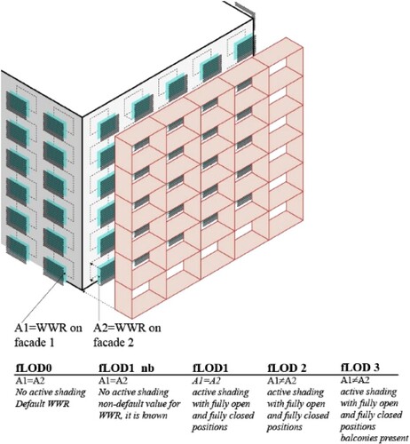
Each façade variant is represented at low and progressively higher fLODs. Figure 2 shows an example massing scheme with various façade elements that are added to it incrementally at each fLOD. Low fLOD (fLOD0) indicates that no façade design information is available and the 3D model only relies on assumed and minimal façade inputs that are all subject to change later on. Higher fLODs (up to fLOD3) addressed in this study include design decisions related to more refined aspects of the façade, such as window-to-wall ratio (WWR), window area distribution per orientation, and fixed or active shading devices for instance. We provide further detail on the method of generating façade variants in Section 2.2. As mentioned above, three metrics were identified for this study for their relevance to early design stage decisions and their compatibility with the current status of use in BPS (well-established, easily accessible existing workflows for their calculation), namely: spatial Daylight Autonomy (sDA), annual heating and annual cooling demand. Further explanation regarding the choice of metrics and of the modelling methods used for converting 3-D geometry at various fLODS into BPS models is provided in Section 2.3.

Figure 2. Exploded view showing incremental levels of façade detail at which 3D models are produced by the grasshopper workflow.

2.1.2. Pairwise comparison of two given massing-schemes

Next, we compare two massing-schemes that would potentially be competing with one another in a hypothetical decision-making process. While it is common to have more than two competing design proposals at the early design stage, comparing options two-by-two (pairwise comparison) is the simplest form of ranking exercise and will be used in this paper. The two design alternatives are thus ranked based on performance on a given metric (e.g. sDA) and one of them is either identified as the preferred scheme or both are proclaimed as equivalent because the difference in performance is negligible.

2.1.3. Calculation and characterization of risk due to unknown design decisions to be made at higher fLOD

The loss in performance due to any disagreement in choice of massing scheme at low versus high fLOD is then estimated. The risk of performance loss is calculated using Opportunity Loss (Savage 1951) described in further detail in Section 2.4. We also propose a strategy for identifying cases where the risk of loss is high enough for remedial action to be considered essential (Section 2.5).

2.1.4. Estimation of prevalence of high risk in early design performance evaluations

By repeating the process mentioned above with several pairs of massing scheme proposals, we assess the general level of caution that should be associated with making massing-scheme-related design decisions based on the performance values observed at low fLOD. This step is further detailed in Section 3.

In summary, the proposed methodology allows one to:

• assess the risk of performance loss when choosing what appears to be a higher performance neighborhood massing-scheme at low LOD.

• identify ‘high’ risk cases to determine the suitability of conceptual neighborhood massing models for BPS assessments.

• estimate the risk of performance loss due to a poor choice of massing-scheme at the conceptual design stage (low LOD).

2.2. Development of 3-D models at various fLODS

The conversion of 3-D massing models from fLOD0 to fLOD3 was done using a script in the grasshopper plug-in for Rhino 5.0. An asset of the grasshopper workflow is that it maintains continuity of the design process and geometrical hierarchies between building elements when generating higher fLOD variants. At fLOD0, window openings are present but the area is assumed to be unknown to the designer; therefore, a default value of 30% for the window-to-wall ratio was used. As a first step forward from fLOD0, the WWR is decided upon by the designer which may be more than, less than or equal to the default value. This is followed by the window placement. Once the window distribution is determined, the balconies, the balconies are placed accordingly (facing glazed doors, which are also considered as windows).

More explicitly, five steps are followed to arrive at fLOD3 variants from fLOD0:

1. At fLOD0 windows are input as simple punched windows (30% WWR), uniformly distributed on all faces, all with the same height and sill height (2 and 0.75 m respectively). The number of windows per face is estimated based on the number of apartments per floor. Once this number is determined at fLOD0 for a particular massing-scheme, it is kept the same at all fLODs.

2. In the second step, three variants are created, with three possible values (20%, 30%, 40%) of WWR. Each WWR is used to revise the total resulting glazed area, which is then distributed uniformly again on all vertical faces of the massing-scheme same as fLOD0. The window height and sill height are kept unchanged.

3. In step 3, active shading devices are added in the form of shading schedules (on/off type) to be used in annual daylight and dynamic thermal simulation models.

4. In the fourth step, we deviate from a uniform distribution of glazing on all faces to reflect a designer's intent to identify primary and secondary façades. If the secondary façade carries any glazing, the WWR is at least 10%. The remaining glazed area is assigned to the prominent façade. Four variants are modelled at each WWR value, one where the prominent façades are those with a high sky view factor (SVF), second where prominent façades are those with a low SVF, third where prominent façades face either east or south, and fourth, where prominent façades face either west or north. Active shading operation schedules are updated (still in on/off mode) in step 4 to account for this new distribution of glazing. At this fLOD, we will have generated 12 façade variants (3 * 4).

5. In the final step, we arrive at fLOD3. Four possible balcony types are assigned here to the prominent façade (identified in step 4). Active shading operation schedules are updated again to account for the addition of balconies (fixed shading devices). Please refer to Appendix A for more details about the active blind modelling method used. At this final fLOD, we end up with 48 façade variants per massing-scheme (3 * 4 * 4)

A limited number of façade design variants (48) have been considered here out of the seemingly infinite plausible façade designs for a given massing scheme. The number of variants was limited to a point where satisfactory number of pairwise comparisons could be done between façade variants of two competing massing schemes and meaningful value of risk could be reported. In other design contexts if a wider variety in façade design solutions is expected and more design details considered relevant to the risk assessment, then the number of variants will need to be re-evaluated.

2.3. Approach for performance evaluation at various fLODS

The building performance metrics for this study were chosen carefully such that they remain possible to calculate irrespective of the level of design development. For example, the Residential Daylight Score (RDS) (Dogan and Park 2017), while more appropriate for residential buildings, was not considered at this time as it requires internal layouts to be present for its calculation. An issue like this could be addressed, for example, by applying a default zoning type to conceptual stage models (Dogan, Reinhart, and Michalatos 2016) which could potentially influence performance just like default assumptions regarding WWR. However, any risk assessment problem requires a reasonable scope or horizon to be defined and we here assume that when making performance-based decisions regarding massing-schemes at the conceptual design stage, a decision maker’s primary interest is likely to be to optimize the solar radiation received at (and conduction gains transmitted through) the building surfaces. Thus, the scope of uncertainty in design details was restricted to building elements that interfere with the intake of solar radiation and the main focus of this paper is kept on developing and demonstrating the risk assessment methodology.

The metrics were also chosen such that they exhibit lower sensitivity (compared to other metrics) to design details that would be well beyond the conceptual/early design stage. For example, the Useful Daylight Illuminance metric (UDI) (Nabil and Mardaljevic 2005) has been shown to be more sensitive to reflectance properties of the interior surfaces compared to sDA (Brembilla, Hopfe, and Mardaljevic 2018). Thus, if the risk of sub-optimal decision making were to be explored using the UDI metric, then the uncertainty in reflectance properties of surfaces must also be included. Specific details and inputs used in generating performance estimates in this paper are provided in the Appendix.

2.4. Decision making and risk of performance loss

Decision-making under uncertainty is an unavoidable aspect of any performance-based design process (Hopfe, LM Augenbroe, and Hensen 2013). The notion of risk, in this context, can thus be considered as a subset of uncertainty that represents conditions of (performance) loss. It is a common tool for decision-making under uncertainty that ignores the ‘upside’ of uncertainty where favourable performance gain may be achieved, and looks instead at the probability and extent of loss if encountered. In this study we assume that the decision maker is not interested in reducing uncertainty: the decision maker just wants to avoid being wrong.

2.4.1. Decision making at low fLOD

As introduced in Section 2.1, the objective of the proposed process is to assess the suitability of massing-schemes for evaluating performance at an early design stage of design, i.e. at a low fLOD. The decision-making process starts with a given pair of neighbourhood massing-schemes, that we will refer to as schemes A and B. At this point, the decision maker is expected to choose one massing-scheme over another only if an appreciable performance difference is observed between them. This appreciable difference is interpreted as a decision criterion (dc) for a decision maker to rule in favour of one design over the other.

For the purpose of the present paper, we chose to establish the dc based on existing standards, and considered a difference to be significant if it was likely to get the performance to a different score or level based on the standard (applies to annual heating and cooling demand), or, when lacking such a reference, was typically understood to be a significant change on the said metric (applies to sDA). Table 1 shows the selected levels of decision thresholds.

Table 1. Possible values for decision criteria for various performance metrics.

Metric	Minimum performance differentiation
sDA (daylight)	10% (sDA units) improvement in sDA is generally considered to be a minimum appreciable difference between design alternatives (Iversen, Svendsen, and Nielsen 2013)
Annual Heating Demand	2.8 kWh/m2-year (reduction in annual heating demand needed to upgrade from code compliant (SIA 2017) to MINERGIE-P rating (MINERGIE 2022))
Annual Cooling Demand	3.8 kWh/m2-year (reduction in annual cooling demand needed for upgrading comfort Category III to Category II (ISO 2005))

When a preferred scheme is identified at low fLOD, we notify this event as (A*, B) where A is the preferred massing-scheme. We assume that if a performance difference greater than or equal to dc is not seen, the decision maker would be indifferent and could choose either scheme, in which case (A*, B) and (A, B*) would be considered equally likely to occur.

2.4.2. Measurement of risk

Su and Tung (2012) extended the interpretation of opportunity loss for design and engineering problems using pair-wise comparison of possible decision outcomes. This measure is called Expected Opportunity Loss (EOL) (Su and Tung 2012). Under this approach, only equivalent façade variants of massing Scheme A would be compared to those of Scheme B (Figure 3). We shall refer to this as a peer-to-peer comparison.

Figure 3. Diagram showing multiple design variants emerging at each level of detail. Two fLOD3 variants of the massing schemes A and B are considered comparable peers of each other if the designer would make similar design choices (indicated by branches with arrows) to arrive at them (e.g. same WWR, same balcony type).

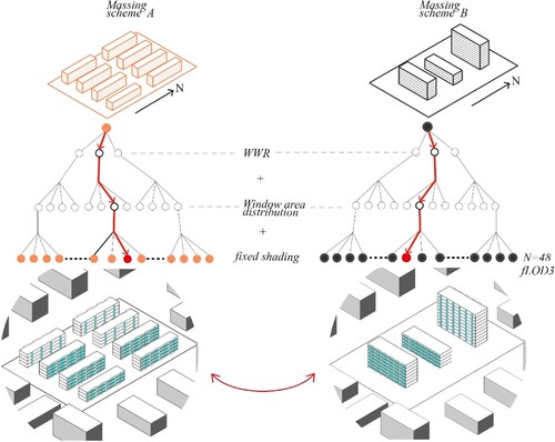
When the 48 high fLOD variants of the two massing-schemes A and B are compared, 192 valid peer-to peer comparisons are produced (48 * 4 = 192), allowing for cross-comparison between orientation-related variants. We thus derive the relative performance difference between the two-given massing-schemes as a distribution with N = 192.

The Expected Opportunity Loss (EOL) is expressed as in equation 1(1) $\mathrm{EOL}(A^{\ast },B)=-\underset{-\mathrm{\infty }}{\overset{0}{\int }}f\mathrm{\Delta }(A^{\ast },B)\mathrm{d\delta }(\mathrm{Su}\mathrm{and}\mathrm{Tung}2012)$(1) : (1) $\mathrm{EOL}(A^{\ast },B)=-\underset{-\mathrm{\infty }}{\overset{0}{\int }}f\mathrm{\Delta }(A^{\ast },B)\mathrm{d\delta }(\mathrm{Su}\mathrm{and}\mathrm{Tung}2012)$(1) where EOL (A*, B) is the Expected Opportunity Loss when A is the preferred massing-scheme at low fLOD, and $f\mathrm{\Delta }(A^{\ast },B)$is a probability distribution function (PDF) of the relative performance gain from design pairs formulated at the highest fLOD.

Expected Opportunity Loss was further interpreted in three different types of conditions:

• Opportunity loss due to rank reversal This is the type of opportunity loss that a decision maker is likely to be most averse to, where the performance-based ranks assigned to massing-scheme options (at low fLOD) carry a high risk of being overturned or reversed at high fLOD. A pre-requisite for this type of opportunity loss is that the decision maker is able to establish clear ranks at fLOD0 with the observed performance difference between the two massing-schemes being greater than dc. In this case the EOL is expressed in equation1.

• Opportunity loss due to latent performance gain Rank reversal is the most serious error in decision making where, due to insufficient level of detail, the findings at low fLOD are overturned at higher fLOD. However, other forms of loss are also worth considering. If the decision maker decides to not assign ranks to the design options at low fLOD due to insufficient difference in performance, loss may still be incurred if the decision maker is failing to identify a better performing design solution due to low fLOD. In case the decision maker observes insufficient performance gain between (A, B) at low fLOD, he/she considers both (A*, B) and (B*, A) to be equivalent, and there is only a 50% chance that he/she will choose the massing-scheme that does yield higher performance later on. This form of loss is analogous to the higher partial moment where more than anticipated gains can be achieved later but would remain hidden or latent unless the performance comparison is done at higher fLOD. Opportunity loss in this case could be expressed as follows (equation 2(2) $\begin{array}{rl}\mathrm{EOL}(A,B)& =-(0.5X{\int }_{\mathrm{dc}}^{\mathrm{\infty }}f\mathrm{\Delta }(A^{\ast },B)\mathrm{d\delta }\\ & +0.5X{\int }_{\mathrm{dc}}^{\mathrm{\infty }}f\mathrm{\Delta }(A,B^{\ast })\mathrm{d\delta })\end{array}$(2) ): (2) $\begin{array}{rl}\mathrm{EOL}(A,B)& =-(0.5X{\int }_{\mathrm{dc}}^{\mathrm{\infty }}f\mathrm{\Delta }(A^{\ast },B)\mathrm{d\delta }\\ & +0.5X{\int }_{\mathrm{dc}}^{\mathrm{\infty }}f\mathrm{\Delta }(A,B^{\ast })\mathrm{d\delta })\end{array}$(2) where EOL (A, B) is the EOL when A or B could be chosen with equal probability at fLOD0 and $f\mathrm{\Delta }(A^{\ast },B),f\mathrm{\Delta }(A,B^{\ast }),$are the probability distribution functions of the relative performance gain from design pairs formulated at the highest fLOD.

• Opportunity loss due to insufficient performance gain This form of loss is not associated with making a sub-optimal design choice (choosing a lower performing design alternative), but one where the anticipated performance gain, on the basis of which a preferred massing-scheme is identified (A*, B) at fLOD0, is not realized later. This is also called the lower partial moment and is used as risk measure when less than desired performance is achieved (Bawa and Lindenberg 1977): (3) $\begin{array}{rl}& \mathrm{EOL}(\mathrm{dc},\mathrm{RPG},(A^{\ast },B))\\ & =-{\int }_{\mathrm{dc}}^{\mathrm{\infty }}(\mathrm{dc}-\mathrm{rpg})f(\mathrm{rpg})\mathrm{d\delta }(\mathrm{Su}\mathrm{and}\mathrm{Tung}2012)\end{array}$(3) where EOL(dc, RPG,) is the Expected Opportunity Loss when dc is the minimum desired relative performance differentiation, RPG is the distribution of the relative performance gains when massing-scheme A is chosen as the preferred scheme and $f(\mathrm{rpg})$ is the probability distribution function of RPG.

2.5. Characterizing risk as ‘high’ or ‘low’

In the previous section, three different forms of opportunity loss are described that could occur and could be important to a BPS user. We present the sum of the total risk from all possible forms of opportunity loss as a single joint value, the Expected Relative Performance Loss (ERPL). While the definition of EOL may be adapted to address different types of losses (e.g. loss equation 1(1) $\mathrm{EOL}(A^{\ast },B)=-\underset{-\mathrm{\infty }}{\overset{0}{\int }}f\mathrm{\Delta }(A^{\ast },B)\mathrm{d\delta }(\mathrm{Su}\mathrm{and}\mathrm{Tung}2012)$(1) versus loss equation 3(3) $\begin{array}{rl}& \mathrm{EOL}(\mathrm{dc},\mathrm{RPG},(A^{\ast },B))\\ & =-{\int }_{\mathrm{dc}}^{\mathrm{\infty }}(\mathrm{dc}-\mathrm{rpg})f(\mathrm{rpg})\mathrm{d\delta }(\mathrm{Su}\mathrm{and}\mathrm{Tung}2012)\end{array}$(3) ), it is difficult to anticipate which type of loss may be encountered in a given decision making situation. ERPL is proposed for decision makers who are interested in avoiding loss irrespective of its nature (loss from rank reversal, latent performance gain or insufficient performance gain). The ERPL value has the same units as the metric value which is being used to compare the design alternatives. The detailed calculation method of ERPL is further illustrated in Section 3.2 with an example.

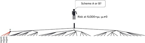
It should be noted here that risk is probabilistic in nature and high values of risk do not imply that an incorrect decision will be made. Similarly, low risk does not guarantee a loss free decision. Consider a decision maker (DM) about to make a choice. The DM, while deciding between two design alternatives A and B, encounters some risk of sub-optimal decision making (µ₀) (see Figure 4). In this case, the risk is emanating from regret if the façade design evolves in a certain manner at fLOD3 (shown as ‘child’ designs of node ‘n’ in Figure 4). However, the DM does not know if he/she will end up on the node ‘n’ of this decision tree and then if the risk is applicable to him/her. To resolve this, a simple rule/strategy is proposed that sets a risk threshold value for the risk at the beginning of the design process such that the possibility of going down on an extremely adverse future design path can be averted: an adverse design path is called so if more than 50% paths downstream from it lead to regret. It is assumed that the DM is not interested in eliminating loss completely (in that case, maximum acceptable risk would be zero), but rather lower it to a safe limit.

Figure 4. Diagrammatic representation of sequential decision making and strategy-based risk management. Black lines indicate possible paths of design development leading to no regret. Red lines indicate paths leading to regret. Each node in the tree represents an additional design detail being specified.

Using the methodology described in Section 4.1–4.3, we evaluated the effectiveness of selecting a massing scheme based on simulations results at low fLOD. To do so, we apply the risk assessment methodology to a number of massing-scheme pairs and estimated the incidence rate or prevalence of high-risk cases.

3. Experimental estimation of risk: A case of medium density Swiss neighbourhood design

In order to estimate the incidence of high risk in conceptual stage design decisions, a hypothetical design problem was used in which a residential neighbourhood is to be developed at a density of 1.0 on a plot of 15,000 m2. It was further assumed that the design team follows an ‘outside in’ approach where ‘the building form is developed and once a basic building form has been conceived, different façade variants can be explored’ (Reinhart and LoVerso 2010) (i.e. the designer chooses the massing scheme first and explores façade design later).

Different design development approaches (e.g. inviting proposals for massing schemes via design competitions or detailed design development under a master plan) may result in different set of competing massing scheme proposals. The competing massing scheme proposals may share some important traits with each other (e.g. same orientation of buildings, number of buildings) or they could also have contrasting characteristics that offer complementary advantages. For example, one scheme could be better aligned with the prevailing wind direction and the competing proposal may offer better views to occupants. In this study we considered two scenarios (1) different design teams develop the competing design proposals and so the design proposals are not bound to have any common design concept or traits (2) there is one design team and it is working on a specific design concept. Competing design proposals thus share at least one important design trait.

To generate a large number of instances of decision making under the two scenarios mentioned above, a set of massing-schemes (N = 40, shown in Figure 5) was developed manually, serving as a pool of potential design proposals on the given site. All massing-schemes proposals had the same volume and floor area (+/−1%). Geometrical properties (e.g. type of building arrangement on site, number of buildings) of the massing scheme proposals were systematically varied in the generation of this set to create a wide range of design possibilities. The built context around the site was modelled at the same density as the design site (cf. Figure 1) and held constant across all design variants. Under the first scenario (no single defined design concept), we repeatedly drew two schemes at a time from the entire pool of 40 massing schemes to generate comparisons and each pair became an instance of decision making. Under the first scenario we thus ended up with 780 ($C_2^{40}$ = 780) performance comparisons between potentially competing design options on the three metrics (sDA, heating demand and cooling demand). As an example of the second scenario, we assumed the design team chose to work with only a specific type of arrangement of buildings on site (e.g. courtyard arrangement, see Figure 5). The team in that case could be comparing, for example, scheme D to scheme D1 or A to A1 (Figure 5). Another type of common design trait could be that the building depth where the depth of the floor plate is kept same across all design variants, and thus, as examples, the team could have schemes E1 and D1 or E1 and A1 (Figure 5) as competing design proposals.

Figure 5. Example set of massing-schemes (total number of schemes = 40) for a given site. Five different types of site arrangements were attempted: regularly spaced buildings, regularly spaced buildings but varying heights, clustered buildings creating open spaces, courtyard and horizontally staggered arrangement.

We applied the methodology discussed in Section 2 to each comparison so as to calculate the risk of performance loss, and then identified all high-risk cases. Out of the numerous pairs of competing massing-schemes that were generated, we chose two pairs of massing-schemes from the first scenario to illustrate the workings of the methodology for calculation of risk of an incorrect decision being made. The pairs shown are those where appreciable opportunity loss was observed on at least one of the metrics. They are indicated as massing-schemes A, B, C and D in Figure 5 (it may be noted that scenarios A and B are consistent with those shown in Figure 3 as well).

3.1. Example comparisons of massing-schemes at early design stage

The raw performance values from simulations at fLOD0, fLOD3 and the intermediate steps are shown for massing-scheme pairs (A, B) and (C, D) in Figure 6. The overall shaded regions show the range of performance possibilities at each fLOD. The sub-regions in darker shade show performance values for the pair of schemes at a particular WWR. While Figure 6 does not clearly show all conditions of loss, as those can only be observed when the peer-to-peer or pairwise comparison between façade variants is done, the figure indicates if there is a potential overlap in performance among peer fLOD3 variants or not. On the sDA metric, in the comparison between schemes A and B, we see high chances of rank reversal at fLOD1 and after.

Figure 6. (Left Column) Evolution of performance of design options A, B shown in Figure 5, on three metrics (1) sDA, shown on top (2) Annual Heating Demand, middle (3) Annual Cooling Demand, bottom. The highlighted regions show evolution of performance values when ‘low’ WWR (20%) is decided upon by the designer at fLOD1. (Right Column) Evolution of performance of design options C, D shown in Figure 5 on three metrics in the same order as column on left. The highlighted regions show evolution of performance values when ‘high’ WWR (40%) is decided upon by the designer at fLOD1.

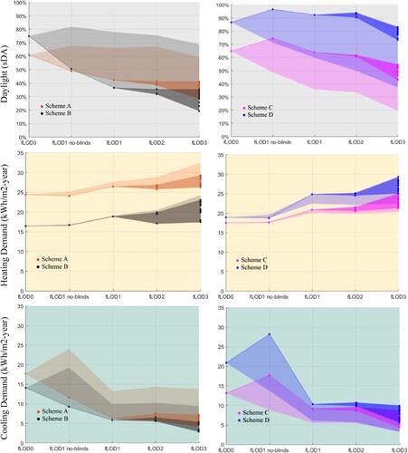
We can tentatively observe the latency effect in the evolution of heating demand evaluation for schemes (C, D) where the performance difference between C and D is negligible at fLOD0 but becomes significantly larger at fLOD3. On cooling demand, in both pairs of evaluations, we see that the performance of both design options converge, and thus it is likely that an appreciable difference in performance will not be not observed at fLOD3. Note that the observed performance difference at fLOD0 is diminished significantly after inclusion of active shading at fLOD1.

3.2. Example calculation of risk of performance loss

Out of the two pairs presented above, we further selected pair (A, B) to illustrate the calculation of the expected risk of relative performance loss (ERPL). Figure 7 shows a subset of the peer-to-peer comparison in the strictest sense at fLOD3. To conserve space, all possible combinations (192) are not shown. That is, in these pairs, the WWR, the orientation of the prominent façade and the balcony type are the same. Figure 8 shows the probability density of relative performance differences found at fLOD3.

short-legendFigure 7.

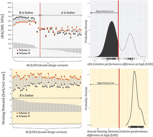
Figure 7. Relative performance comparison for massing-scheme A,B at fLOD3 shown when strict one-to-one pairing is done for the 48 design variants at FLOD3. The comparisons to the right of the vertical dotted line (if present) reflect opportunity loss due to rank reversal.

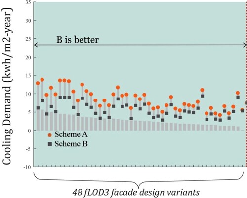
Figure 8. Probability density of relative performance values (A-B) at high fLOD (fLOD3) when a cross comparison between patterns of distribution of glazing on facades is permitted. Area under the curve to the left of the solid vertical line is equal to the Expected Opportunity Loss

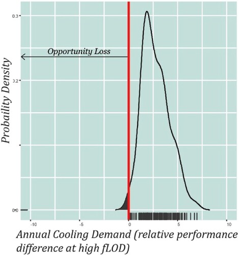
On sDA, a difference of 13.94% is observed between schemes A and B at fLOD0 (Figure 6, top-left). If the decision maker’s decision criterion is a 10% difference, then the DM would choose scheme B based on daylight performance evaluation at fLOD0. However, Figure 8(a) shows that the negative half of the distribution (i.e. design possibilities resulting in A performing better than B) is substantial. The shaded part of the area under the curve (Figure 8(a)) represents the expected relative performance loss, which in this case was found to be 4.4% (in absolute units i.e. difference in sDA). This could be interpreted as a 44% chance that the performance of scheme B will be 10% worse (in sDA units) compared to A when considering all possible façade design solutions at fLOD3. Based on the method described in Section 2.5, the risk threshold for the sDA metric was found to be 2.1% and as a result we would assess this comparison between A, B on sDA at fLOD0 as high risk. While the overall probability of 44% is less than an even chance (50/50), this risk is not evenly distributed on all future design paths. The low WWR scenario, illustrated by the highlighted region in Figure 6(a), shows a high chance of rank reversal and this condition is captured by the risk threshold-based decision-making strategy.

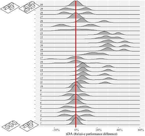
3.3. Prevalence of high risk at fLOD0

The process described above was repeated for all pairs of competing massing-schemes. For illustrative purposes, Figure 9 shows the probability density for an example set of 30 comparisons on the sDA metric. The ERPL is calculated for each comparison and compared to the high-risk threshold value for each metric. We record all high-risk cases and the loss (if any) incurred from each pair of massing-scheme comparisons. If we look at the first scenario, where there was no specific and shared design concept (or design traits) between the design proposals, on sDA, we found 22% of the comparisons at fLOD0 to be high risk (assuming dc = 10% for all comparisons).

Figure 9. Probability density of relative performance values (A-B) at high fLOD (fLOD3) 30 neighbourhood comparisons. Area under the curve to the left of the solid vertical line indicates possible Expected Opportunity Loss.

Further under the first scenario, 1 out of 7 comparisons on heating demand (with dc = 2.8 kWh/m2-year) and 1 out of 12 on cooling demand (with dc = 3.8 kWh/m2-year) were found to be high risk. Note that the risk/expected loss value calculated here is an average value given a wide range of façade design possibilities and does not indicate a maximum possible loss due to the incorrect choice. Also, these risk values result from the exclusion of selected façade details from conceptual stage models (cf. Section 2.3) and the effect of other missing design details is currently ignored.

Table 2 shows results from two example situations under the second scenario, where the competing design proposals share a common concept. The design concept or trait, whether selected by the design team or imposed by the master plan, will imply that all competing massing schemes share important similarities. Comparing similar schemes did not appear to necessarily mitigate risk of incorrect decision making. For example, comparing only ‘courtyard’ type schemes (Scenario 2a, Table 2) where building facades are oriented in varied directions, appeared to reduce the risk of incorrect decision at fLOD0. However, in scenario 2b (Table 2) for example, if the design team chose to only work with a building depth of 10 m or less, then the evaluations were found to be risker on daylight and cooling demand metrics. Higher fLOD would be more suitable for making decisions under such a situation.

Table 2. Risk of erroneous decision making when performance is evaluated at low fLOD.

		Number of high-risk cases in decision making when comparing a pair of massing schemes (n, (% of high risk cases))
Decision making scenario	Number of pairs of massing schemes	Daylight access (sDA)	Heating demand	Cooling demand
Scenario 1: All types of schemes are considered comparable to each other	780	172, (22%)	117, (15%)	65, (8.3%)
Scenario 2a: Design concept based the type of massing schemes (e.g. courtyard schemes only, schemes like D and D1 compared to each other in Figure 5)	45	8, (17.7%)	2, (4.4%)	3, (6.6%)
Scenario 2b: Design concept where the building depth is kept constant (e.g. Schemes such as A1 compared to schemes like B1, C1, D1 or E1in Figure 5)	36	10, (27.7%)	2, (5.5%)	22, (48.8%)

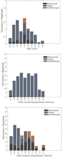
Another characteristic of the risk, apart from incidence rate, is the source of the risk. Figure 10 shows the cumulative ERPL by order of magnitude of the ERPL (x-axis) for each metric from the 780 neighbourhood comparisons done in this study. The source of the performance loss is indicated by colour. In decisions based on sDA and annual cooling demand, all three types of losses were found, while in heating demand-based decisions, in most comparisons where any loss was found, it was due to the latency effect. That is, loss in heating demand-based decisions was mostly found to occur in cases when the performance difference between two massing-schemes appears to be negligible or insignificant at fLOD0. and increasing the fLODs tended to amplify the performance difference between two schemes.

Figure 10. Distribution of risk of performance loss at fLOD0 (ERPL at fLOD0) observed in 780 comparisons. Source causes of performance loss indicated by colour (a) sDA, top (b) Annual Heating Demand, middle (c) Annual Cooling Demand, bottom.

4. Discussion

4.1. Interpretation of findings

Many recent studies have specifically addressed BPS users while proposing various techniques for robust decision making. Yet, their use in practice remains low. This study generates evidence in support of using robust decision-making practices especially when using BPS tools at the conceptual design stage. High risk of incorrect decision making was found in 22%, 15% and 8% of the 780 pairwise comparisons of massing schemes on sDA, annual heating and cooling demand evaluations, respectively. These findings suggest that the value of conceptual stage design decisions is not the same across performance metrics. Thus, daylight potential, based on early design sDA calculations (fLOD0 models), was found to be least reliable for decision making compared to heating and cooling demand-based assessments.

Taking the example of the most critical metric here i.e. sDA, with 22% erroneous cases (or 1 in 5 chance of erroneous decision) basically means that if a design firm typically produces two design alternatives at the conceptual design stage and works on five or more neighbourhood scale projects in a year, it can expect to make an erroneous decision on one of these projects based on sDA values obtained from fLOD0 models.

This study also proposes a new risk metric (ERPL) for the sequential design process where the decision maker makes choices based on relative performance of the design alternatives at a given point in time (massing-design). The risk estimation method for calculating ERPL has been further extended to identify cases where the risk is ‘high’ enough to trigger remedial actions by the decision. Remedial actions imply additional design effort or time, for example, additional time needed for delaying the decision or gathering more design information to reduce uncertainty in performance estimates. This risk assessment methodology tries to find balance between design time and robustness. A given decision is called ‘high’ risk only when the regret/opportunity loss is unacceptable to the decision maker (and not simply greater than zero) and the likelihood of experiencing regret is also unacceptable (e.g. more than 50% chance). The thresholds of unacceptability can be altered in different contexts by different users.

4.2. Implications on use of BPS tools in building design

While risk assessment is common practice in several disciplines related to building design (e.g. structural design), it is virtually absent in use of BPS tools (Clarke and Hensen 2015; Østergård, L Jensen, and Maagaard 2017). This study reports risk in decision making, in terms of model LOD (more specifically fLOD), a construct that many architects and designers are familiar with. The framework presented in this paper thus offers the potential to add important qualifiers to reported performance values from BPS tools, namely, the current fLOD of BPS model and the resulting risk in decision making.

At the same time, the proposed risk assessment does imply a greater computational burden on the conceptual stage decision maker. On projects where BPS is being utilized mostly for compliance purposes, carrying out a risk assessment involving multiple future design scenarios maybe considered as excessive. When undertaking large projects in which a number of design alternatives are being considered (for example, multiple entries to a neighbourhood scale design competition), the incremental cost of the risk assessment maybe justified, given the larger effort (design time, cost) invested in generating multiple alternatives.

Well-intentioned design constraints (e.g. narrow section buildings) can deliver better performance on multiple metrics but may not mitigate risk in decision making. Increasing reliability in decision making and choosing design attributes that support performance goals can thus be seen as two different aspects of the performance-driven design process.

The concepts of ‘performance-gap’ (Menezes et al. 2012) and ‘design-gap’ (Wright, Nikolaidou, and Hopfe 2016) have been created to bring accountability in the use of BPS tools in the design process through the use of better modelling practices and design space exploration methods. This study shows that the quest for greater accountability would be incomplete without a critical examination of the decision-making practices.

4.3. Limitations and potential future extensions

Our findings regarding the prevalence of high-risk cases at the early design stage are a unique aspect of this study. Several studies so far have been grounded in the general assumption that early design decisions are important and that the built form sets the course for the performance potential that can eventually be met by the project. This study shows that in order to capitalize on the performance potential available at the conceptual design stage, robust decision-making methods are needed. At the same time, prevalence rates of incorrect decision making that are reported here are closely related to the context and scope of the study, especially the density (1.0) and location (Geneva, Switzerland). Generalizations to different contexts could require further investigations.

In addition, the reported prevalence of risk calculated using ERPL is based on a number of assumptions regarding constructs like ‘acceptable loss’ and ‘decision criterion’ which have not been formally investigated among BPS users. The structure of the ERPL metric also currently assumes that all enumerated future courses of design development at the detailed design stage are equally plausible and then reports the risk. The relevance of the ERPL metric to its users can be further enhanced by assigning probabilities (for e.g. based on cost of construction) to future design development scenarios.

The LOD framework used in the study can also be extended to include exterior elements on the site (e.g. trees, hardscape elements) and interior details such as interior partitions. Such extensions would allow for risk assessment on more metrics and meaningful consideration of more passive design strategies. For example, natural ventilation, and night time ventilation are effective passive cooling strategies in residential buildings that are tied to the massing and façade design. However, for modelling airflow in and around building, interior wall partitions are also needed which have been currently excluded (also see Section 2.3) as the aim of this study was to report risk from exclusion of façade details.

5. Conclusions

The main goal of this study was to assess the reliability of BPS-based design decisions made at the conceptual stage if uncertainty in future course of design development is ignored. We addressed this problem at the neighbourhood scale in the context of a typical conceptual stage decision making task – choosing one design out of two given alternatives. A risk metric (ERPL) was developed to report the likelihood and magnitude of performance loss from sub optimal choice resulting from use of simple, low fLOD geometry as the BPS model input. This risk metric reports likelihood of loss due to three potential reasons: performance-based ranking of design alternatives getting disrupted at higher fLOD, loss of performance difference or ranks between design alternatives at higher fLOD or ranks emerging between design alternatives when there were none at low fLOD.

The results show that there is higher risk in relying on performance evaluation on some metrics (sDA for daylight access) than other metrics (e.g. ideal cooling, heating loads). The risk was found in enough instances of decision making (e.g. 1 in 5 high risk cases found in 780 instances of conceptual stage choices between massing schemes based on sDA) to reconsider modelling practices or metrics used at the conceptual design stage.

Using a higher LOD for making critical design decision indicates a more integrated design approach, but also implies additional design/decision making effort. It may not always be possible to align informational needs of BPS models with the design development process. When it is known that the BPS model suffers from information deficiency, even then the presented methodology provides useful information to the decision maker, allowing him/her to understand if a reliable design decision can be made at the current LOD or not.

Typically, the choice of LOD of BPS models is based simply on the amount of design information available at hand. Findings indicate a need to qualify simulation results with model LOD being used and the risk in relying on performance estimates thus far. This paper provides motivation for wider use of available methods for uncertainty analysis by BPS users. Formal development of an LOD framework that is specific to the informational needs of BPS models could increase clarity and transparency.

List of Abbreviations

BPS – building performance simulation

LOD – level of detail

fLOD – façade level of detail

EOL – expected opportunity loss

ERPL – expected relative performance loss

Acknowledgements

The authors would like to thank Dr. Marc-Olivier Boldi for his advice that proved to be critical for the development of this work. The large number of daylight simulations needed for this work were conducted with invaluable support from Dr. Jan Wienold.

Disclosure statement

No potential conflict of interest was reported by the author(s).

Data availability statement

Raw data were generated at the institute servers (ENAC, EPFL, Switzerland). Derived data, supporting the findings of this study are available from the corresponding author MA on request.

Additional information

Funding

This work was conducted at the École Polytechnique Fédérale de Lausanne (EPFL) with additional support from the SECURE (Synergistic Energy and Comfort through Urban Resource Effectiveness) project funded by the CCEM (Competence Center Energy and Mobility).

Appendix

BPS considerations

Modelling scripts in grasshopper have been developed to generate (N = 48) fLOD3 design variants on any given massing-scheme, following the steps described in Appendix B. The conversion of 3-D geometry (from Rhino 5.0) at various fLODS to BPS models was done using grasshopper, ladybug and honeybee suite of plug-ins for Rhinoceros 5.0. Metric specific inputs, modelling protocols and methods followed are described in the Tables below.

In order to ensure that rank changes we observe with the introduction of façade details to massing-schemes occur only due to the intended detail types included in the fLODs, it has been ensured that other design factors (number of window openings, vertical placement and height) remain unchanged. See Table A1 for changes with each fLOD.

Eight DAYSIM simulations were carried out per scenario per fLOD to model blinds in open and closed position per building facade. The eight files were then compiled into one composite illuminance file while applying the blind schedule specific to each building facade, using Matlab. The sDA value was also calculated using Matlab. Radiance simulation parameters input are based on Illuminating Engineering Society (IES) LM-83-12 including indoor and exterior reflectance properties (See Table A2). 5 ambient bounces were used in all simulation where blinds are modelled in fully open position. 6 ambient bounces were used in all simulation where the blinds are modelled in a closed state (as trans material to represent combined transmittance of the closed blinds and the glazing).

IES LM-83-12 standard was followed by and large except for the procedure for modelling of blinds and the density of the illuminance grid. BLINDSWITCH-A (Van Den Wymelenberg 2012) exterior shading manual operation model was used. In this model primary triggers for blind operation are (a) irradiation falling on the exterior surface of window and (b) depth of penetration of direct radiation. BLINDSWITCH-A was considered more appropriate compared to blind operation models based only on incident irradiation thresholds or only based on interior area of floor receiving direct illumination [IESNA 2012]. The sensor grid spacing was set to 1 m by 1 m. This grid size is larger than recommended, but the metric used sDA has been shown to be stable at a grid size of 1 m (Brembilla and Mardaljevic 2019). At fLOD0, no blind operation has been included in line with concerns that many BPS users have at the conceptual design stage regarding simulation time and that too many aspects of the project are unknown for user behavior modelling to be included meaningfully.

All detailed thermal simulations were carried out in EnergyPlus 8.3 (See Table A3 for major inputs). All simulations were run using the solar radiation model ‘FullExteriorWithReflections’ in EnergyPlus that accounts for shadow patterns on exterior surfaces due to detached piece of shading such as over hangs. Exterior reflections were also accounted. However interior distribution of radiation on interior surfaces was not calculated explicitly. Due to the lumped zoning type, more advanced models such ‘FulInteriorAndlExteriorWithReflections’ were not considered necessary either. Monthly heating demand and cooling demand values were extracted. These were converted into annual energy use intensity values using Matlab.

Table A1. Change in inputs for façade variants at each fLOD.

Façade property	fLOD0	FLOD1(no blinds)	FLOD1 with blinds	FLOD2	fLOD3
Façade design attributes
WWR	30%	20%,30%,40%	No change	No change	No change
Distribution of glazed area per facade	Uniform, 30%	No change	No change	Varies 60% to 10%	No change
Active shading	None	None, No change	Manual blind operation	Manual blind operation updated in response to further façade changes at this fLOD	Manual blind operation updated in response to further façade changes at this fLOD
Fixed shading	None	None, No change	None, No change	None, No change	Present, depth varies from 1.2 m-2.4 m
Window size and placement
Number of window units per facade	3 or higher	No change	No change	No change	Same as min – fLOD
Window height	2.0 m	No change	No change	No change	Same as min-fLOD
Window width	0.5 m or higher	No change	No change	No change	Same as min-fLOD model
Sill height	0.25 m	No change	No change	No change	No change except when balconies are present
Glazing properties
visible light transmittance	0.6	No change	No change	No change	No change
SHGC	0.58	No change	No change	No change	No change
U-Value	1.0	No change	No change	No change	No change

Table A2. Daylight simulation inputs.

Daylight Simulation inputs
Location	Geneva, Switzerland
Weather File	Geneva IWEC
Opaque surface reflectance properties
Internal surface of walls	0.5
Internal floor	0.3
Internal ceiling	0.7
Exterior wall surfaces	0.3
Exterior balcony elements	0.3
Ground surface	0.2
Glazing light transmittance
Glazing light transmittance	0.6
Active Shading Properties
Active blinds modelled as trans material to represent closed blinds with 10% light leak and glazing	Trans material properties: 0.06 (glazing + blinds closed) fully diffused transmission
Schedule	Hourly on/off schedule based on (Van Den Wymelenberg 2012)
Simulation parameters
Simulation programme used	DAYSIM 4.0 (C. F. Reinhart 2012)
Sensor array spacing	1 m x 1 m grid
Sensor array height from floor	0.76 m
Ambient bounces	6

Table A3 Yearly dynamic thermal simulation model inputs.

Thermal Simulation inputs
Location	Geneva, Switzerland
Weather File	Geneva IWEC
Envelope properties
Opaque wall U-value (W/m2 K)	0.36
Roof U-value (W/m2 K)	0.4
Glazing U-value	1
Glazing SHGC	0.58
Window-to-wall ratio (WWR)	as per fLOD variant
Exterior reflectance value	0.3
Internal Loads
Internal lighting (W/m2)	6.6
Lighting schedule	Off during unoccupied hours
Miscellaneous equipment (W/m2)	3.0
People density (p/m2)	0.025
Hourly schedules	As per SIA 2024–2015 (SIA 2017)
Occupant Controls
Blind controls	Hourly on/off schedule based on (Nezamdoost and Van Den Wymelenberg 2017)
Fixed shading	as per fLOD variant
HVAC system inputs
Heating setpoint with setback, setpoint (°C)	18, 20
Cooling setpoint with setback, setpoint (°C)	28,25
System Type	Purchased heating and cooling
Ventilation rate	30 m3/h.person
Heat Recovery	not included
Heating/Cooling system efficiency	1
Simulation parameters
Programme used	Energy plus ver 8.4 (Crawley et al. 2001)
Simulation time step	1 h
Shadow calculation frequency	7 days
Solar distribution calculation	Full exterior with reflections
Warm up days	7 days (default)

References

- Agarwal, Minu, Gerald Danseux, Luisa Pastore, and Marilyne Andersen. 2019. Reliability Of Daylight And Energy Demand Evaluations For Decision Making At The Conceptual Design Stage. 16:121–128. Building Simulation: IBPSA.
- AIA. 2019. “Architect’s Guide to Building Performance - AIA.” https://www.aia.org/resources/6157114-architects-guide-to-building-performance.
- ASHRAE. 2018. “Energy Simulation Aided Design for Buildings except Low-Rise Residential Buildings (ANSI Approved) ASHRAE 209-2018.” ASHRAE. https://www.techstreet.com/standards/ashrae-209-2018?product_id=2010483.
- Attia, Shady, Elisabeth Gratia, André De Herde, and Jan LM Hensen. 2012. “Simulation-Based Decision Support Tool for Early Stages of Zero-Energy Building Design.” Energy and Buildings 49: 2–15. https://doi.org/10.1016/j.enbuild.2012.01.028.
- Attia, Shady, and Andre De Herde. 2011. “Early Design Simulation Tools for Net Zero Energy Buildings a Comparison of Ten Tools.” In Conference Proceedings of 12th International Building Performance Simulation Association, 2011.
- Baker, Nick, and Koen Steemers. 1996. “LT Method 3.0 — a Strategic Energy-Design Tool for Southern Europe.” Energy and Buildings 23 (3): 251–256. https://doi.org/10.1016/0378-7788(95)00950-7.
- Basbagill, John P., Forest L. Flager, and Michael Lepech. 2014. “A Multi-Objective Feedback Approach for Evaluating Sequential Conceptual Building Design Decisions.” Automation in Construction 45 (September): 136–150. doi:10.1016/j.autcon.2014.04.015.
- Bawa, V. S., and E. B. Lindenberg. 1977. “Capital Market Equilibrium in a Mean-Lower Partial Moment Framework.” Journal of Financial Economics 5 (2): 189–200.
- BC Housing, BC Hydro, City of Vancouver, City of New Westminister, and Provice of Britsh Columbia. 2018. “BC Energy Step Code – Design Guide.” City of Vancouver, the City of New Westminster, the Province of BC.
- Brembilla, E., C. J. Hopfe, and J. Mardaljevic. 2018. “Influence of Input Reflectance Values on Climate-Based Daylight Metrics Using Sensitivity Analysis.” Journal of Building Performance Simulation 11 (3): 333–349. https://doi.org/10.1080/19401493.2017.1364786.
- Brembilla, E., and J. Mardaljevic. 2019. “Climate-Based Daylight Modelling for Compliance Verification: Benchmarking Multiple State-of-the-Art Methods.” Building and Environment 158: 151–164. https://doi.org/10.1016/j.buildenv.2019.04.051.
- CIBSE, C. O. D. E. 2015. AM11 Building Performance Modelling 2015. London: CIBSE Building Services Knowledge. https://www.cibse.org/Knowledge.
- Clarke, Joseph Andrew, and J. L. M. Hensen. 2015. “Integrated Building Performance Simulation: Progress, Prospects And Requirements.” Building and Environment 91: 294–306. https://doi.org/10.1016/j.buildenv.2015.04.002.
- Compagnon, Raphael. 2004. “Solar and Daylight Availability in the Urban Fabric.” Energy and Buildings 36 (4): 321–328. https://doi.org/10.1016/j.enbuild.2004.01.009.
- Crawley, Drury B., Linda K. Lawrie, Frederick C. Winkelmann, Walter F. Buhl, Y. Joe Huang, Curtis O. Pedersen, Richard K. Strand, et al. 2001. “EnergyPlus: Creating a New-Generation Building Energy Simulation Program.” Energy and Buildings 33 (4): 319–331.
- De Wit, Sten, and Augenbroe Godfried. 2002. “Analysis of Uncertainty in Building Design Evaluations and Its Implications.” Energy and Buildings, A View of Energy and Bilding Performance Simulation at the Start of the Third Millennium 34 (9): 951–958.
- Dogan, Timur, and Ye Chan Park. 2017. “A New Framework for Residential Daylight Performance Evaluation.” BS 2017, San Francisco, USA.
- Dogan, Timur, Christoph Reinhart, and Panagiotis Michalatos. 2016. “Autozoner: An Algorithm for Automatic Thermal Zoning of Buildings with Unknown Interior Space Definitions.” Journal of Building Performance Simulation 9 (2): 176–189. https://doi.org/10.1080/19401493.2015.1006527.
- Futcher, Julie Ann, Tristan Kershaw, and Gerald Mills. 2013. “Urban Form and Function as Building Performance Parameters.” Building and Environment 62: 112–123. https://doi.org/10.1016/j.buildenv.2013.01.021.
- Hester, Joshua, Jeremy Gregory, and Randolph Kirchain. 2017. “Sequential Early-Design Guidance for Residential Single-Family Buildings Using a Probabilistic Metamodel of Energy Consumption.” Energy and Buildings 134: 202–211. https://doi.org/10.1016/j.enbuild.2016.10.047.
- Hoes, P., J. L. M. Hensen, M. G. L. C. Loomans, Bert de Vries, and Denis Bourgeois. 2009. “User Behavior in Whole Building Simulation.” Energy and Buildings 41 (3): 295–302. https://doi.org/10.1016/j.enbuild.2008.09.008.
- Hopfe, Christina J, Godfried LM Augenbroe, and Jan LM Hensen. 2013. “Multi-criteria Decision Making Under Uncertainty in Building Performance Assessment.” Building and Environment 69: 81–90. https://doi.org/10.1016/j.buildenv.2013.07.019.
- Hubbard, Douglas W. 2014. How to Measure Anything: Finding the Value of Intangibles in Business. John Wiley & Sons.
- Huber, Jorg, and Christoph Nytsch-Geusen. 2011. “Development of Modeling and Simulation Strategies for Large Scale Urban Districts.” In Proceedings of Building Simulation, 2011:1753–60.
- IESNA. 2012. “IES LM 83 12 IES Spatial Daylight Autonomy (SDA) and Annual Sunlight Exposure (ASE).” IES LM 83 12. Illuminating Engineering Society of North America (IESNA).
- ISO. 2005. “ISO 7730:2005.” https://www.iso.org/standard/39155.html.
- Iversen, Anne, Svend Svendsen, and Toke Rammer Nielsen. 2013. “The Effect of Different Weather Data Sets and Their Resolution on Climate-Based Daylight Modelling.” Lighting Research & Technology 45 (3): 305–316. https://doi.org/10.1177/1477153512440545.
- JEPlus. 2022. Last Updated 2022. http://www.jeplus.org.
- Jusselme, Thomas, Emmanuel Rey, and Marilyne Andersen. 2018. “An Integrative Approach for Embodied Energy: Towards an LCA -Based Data-Driven Design Method.” Renewable and Sustainable Energy Reviews 88: 123–132. doi:10.1016/j.rser.2018.02.036.
- Kochenderfer, Mykel J. 2015. Decision Making Under Uncertainty: Theory and Application. MIT Press.
- Kotireddy, Rajesh, Pieter-Jan Hoes, and Jan L. M. Hensen. 2019. “Integrating Robustness Indicators Into Multi-Objective Optimization to Find Robust Optimal Low-Energy Building Designs.” Journal of Building Performance Simulation 12 (5): 546–565. https://doi.org/10.1080/19401493.2018.1526971.
- Lempert, R. J. 2019. “Robust Decision Making (RDM).” In Decision Making Under Deep Uncertainty: From Theory to Practice, edited by Vincent A. W. J. Marchau, Warren E. Walker, Pieter J. T. M. Bloemen, and Steven W. Popper, 23–51. Cham: Springer International Publishing.
- Menezes, Anna Carolina, Andrew Cripps, Dino Bouchlaghem, and Richard Buswell. 2012. “Predicted vs. Actual Energy Performance of Non-Domestic Buildings: Using Post-Occupancy Evaluation Data to Reduce the Performance Gap.” Applied Energy, Energy Solutions for a Sustainable World - Proceedings of the Third International Conference on Applied Energy, May 16-18, 2011 - Perugia, Italy, 97 (September): 355–64.
- Minergie P Standard. 2022 “Minergie International.” Accessed December 7, 2022. https://www.minergie.com/.
- Nabil, A., and J. Mardaljevic. 2005. “Useful Daylight Illuminance: A New Paradigm for Assessing Daylight in Buildings.” Lighting Research & Technology 37 (1): 41–57. https://doi.org/10.1191/1365782805li128oa.
- Nault, Emilie, Christoph Waibel, Jan Carmeliet, and Marilyne Andersen. 2018. “Development and Test Application of the UrbanSOLve Decision-Support Prototype for Early-Stage Neighborhood Design.” Building and Environment 137: 58–72. https://doi.org/10.1016/j.buildenv.2018.03.033.
- Nezamdoost, Amir, Kevin Van Den Wymelenberg. 2017. “Blindswitch 2017: Proposing a New Manual Blind Control Algorithm for Daylight and Energy Simulation.” In IES Annual Conference Proceedings. Portland, OR.
- Okeil, Ahmad. 2010. “A Holistic Approach to Energy Efficient Building Forms.” Energy and Buildings 42 (9): 1437–1444. https://doi.org/10.1016/j.enbuild.2010.03.013.
- Østergård, Torben, Rasmus L Jensen, and Steffen E Maagaard. 2017. “Early Building Design: Informed Decision-Making by Exploring Multidimensional Design Space Using Sensitivity Analysis.” Energy and Buildings 142: 8–22. https://doi.org/10.1016/j.enbuild.2017.02.059.
- Ratti, Carlo, Nick Baker, and Koen Steemers. 2005. “Energy Consumption and Urban Texture.” Energy and Buildings 37 (7): 762–776. https://doi.org/10.1016/j.enbuild.2004.10.010.
- Reinhart, Christoph, Timur Dogan, J. Alstan Jakubiec, Tarek Rakha, and Andrew Sang. 2013. “Umi-an Urban Simulation Environment for Building Energy Use, Daylighting and Walkability.” In 13th Conference of International Building Performance Simulation Association, Chambery, France.
- Reinhart, C., and V. LoVerso. 2010. “A Rules of Thumb-Based Design Sequence for Diffuse Daylight.” Lighting Research & Technology 42 (1): 7–31. https://doi.org/10.1177/1477153509104765.
- Rezaee, Roya, Jason Brown, John Haymaker, and Godfried Augenbroe. 2019. “A New Approach to Performance-Based Building Design Exploration Using Linear Inverse Modeling.” Journal of Building Performance Simulation 12 (3): 246–271. https://doi.org/10.1080/19401493.2018.1507046.
- Robinson, Darren, Neil Campbell, W. Gaiser, K. Kabel, A. Le Mouel, Nicolas Morel, Jessen Page, S. Stankovic, and A. Stone. 2007. “SUNtool – A new Modelling Paradigm for Simulating and Optimising Urban Sustainability.” Solar Energy 81 (9): 1196–1211. https://doi.org/10.1016/j.solener.2007.06.002.
- Rysanek, A. M., and R. Choudhary. 2013. “Optimum Building Energy Retrofits Under Technical and Economic Uncertainty.” Energy and Buildings 57: 324–337. https://doi.org/10.1016/j.enbuild.2012.10.027.
- Sattrup, Peter A., and Jakob Strømann-Andersen. 2013. “Building Typologies in Northern European Cities: Daylight, Solar Access, and Building Energy Use.” Journal of Architectural and Planning Research 30 (1): 56–76.
- Savage, L. J. 1951. “The Theory of Statistical Decision.” Journal of the American Statistical Association 46 (253): 55–67. https://doi.org/10.1080/01621459.1951.10500768.
- Sefaira. 2022. Last updated 2022. https://www.sketchup.com/products/sefaira.
- SIA. 2017. “Construction Durable Batiment Norme de Comprehension a La Norme SIA 112.” Société suisse des ingénieurs et des architectes(SIA).
- Souza, Clarice Bleil de. 2009. “A Critical and Theoretical Analysis of Current Proposals for Integrating Building Thermal Simulation Tools Into the Building Design Process.” Journal of Building Performance Simulation 2 (4): 283–297. https://doi.org/10.1080/19401490903349601.
- Su, Hsin Ting, and Yeou Koung Tung. 2012. “Minimax Expected Opportunity Loss: A New Criterion for Risk-Based Decision Making.” The Engineering Economist 57 (4): 247–273. https://doi.org/10.1080/0013791X.2012.729875.
- Tregenza, P. R. 2017. “Uncertainty in Daylight Calculations.” Lighting Research & Technology 49 (7): 829–844. https://doi.org/10.1177/1477153516653786.
- Van Den Wymelenberg, Kevin. 2012. “Patterns of Occupant Interaction with Window Blinds: A Literature Review.” Energy and Buildings 51: 165–176. https://doi.org/10.1016/j.enbuild.2012.05.008.
- Wald, Abraham. 1950. Statistical Decision Functions. Statistical Decision Functions. Oxford: Wiley.
- Wright, Jonathan, Elli Nikolaidou, and Christina J Hopfe. 2016. “Exhaustive Search; Does It Have a Role in Explorative Design.” In BSO2016, 3rd Building Simulation and Optimization Conference, Newcastle, UK, September 12. Vol. 14.
- Xia, Chunhai, Yingxin Zhu, and Borong Lin. 2008. “Building Simulation as Assistance in the Conceptual Design.” In Building Simulation. Springer.