Informing building retrofits at low computational costs: a multi-objective optimisation using machine learning surrogates of building performance simulation models

Abstract

Machine learning (ML) algorithms are increasingly used as surrogates for building performance simulation (BPS) models to leverage their energy predictive capabilities while reducing computational costs. In parallel, researchers are developing optimisation methods to inform building design and retrofit strategies but rarely employ ML-based BPS surrogates for this purpose. This study proposes a coupled modelling approach that leverages the capabilities of ML-based BPS surrogate models and multi-objective optimisation to inform holistic design and operation retrofits at low computational costs. The proposed methodology is demonstrated using an archetypal office building in Ottawa, Canada. The developed models achieved competitive predictive accuracies (adjusted R²: 0.90–0.99), identifying total and peak energy saving measures with up to 34% improvement in occupant thermal comfort at computational speeds 1266 times faster than a traditional BPS-based optimisation approach. Results offer a promising modelling workflow for design applications requiring extensive computations and scenario analyses, such as net-zero energy retrofits.

KEYWORDS:

• Building performance simulation
• surrogate modelling
• machine learning
• multi-objective optimisation
• design
• retrofitting

1. Introduction

1.1. Background

Many countries are currently adopting long-term goals aiming to reduce energy consumption in buildings, both for economic reasons and to mitigate the effects of climate change. Canada, for example, aims to achieve net-zero and climate-resilient buildings by 2050 (Natural Resources Canada 2022). In alignment with this aim, Canada has identified building retrofits as a necessary component of this push, which motivated the commissioning of a report on the topic of alterations to existing buildings (National Research Council Canada 2020). To aid this goal and similar goals set out by governments around the world, researchers have worked to advance a myriad of topics relating to building retrofitting as well as energy demand and supply optimisation (Li and Wen 2014; Mariano-Hernández et al. 2021; Shaikh et al. 2014). One such topic is the retrofitting of office buildings, which constitute one of the largest energy consumers amongst commercial/institutional buildings according to the Major Energy Retrofit Guidelines published by the Canadian government (Natural Research Council Canada 2018).

In order to best assess office buildings in need of retrofits, as well as to gauge the effects of certain retrofit strategies on a particular building, many researchers resort to using Building Performance Simulation (BPS) as a powerful physics-based modelling tool capable of assessing a large assortment of retrofit strategies in order to compare and contrast what is most suitable for the building in question. For instance, Bell (2023) surveyed the office building stock in Australia while also developing retrofit strategies for such offices to account for future climate scenarios using BPS tools. Results showed that retrofitting could drive significant energy reduction (13–45%). Daly, Cooper, and Ma (2018) qualitatively studied the usage of BPS for assessing low-performing office buildings in Australia. The authors highlighted the limitations of using BPS for this aim but found that simulations are regularly used to inform retrofitting processes due to poor data availability on such buildings. Finally, Yang and Liu (2018) studied the integration of BPS and BIM tools for optimising retrofits for offices in the colder regions of China. The findings indicated that such an approach proved useful in balancing occupant comfort, environmental impacts, and architectural aesthetics when optimising retrofits for China’s contemporary building stock.

BPS tools such as EnergyPlus can accurately represent building systems and their energy performance. However, BPS simulations are often time-consuming, particularly when dealing with a multitude of designs, such as optimisation of net-zero energy buildings. The stated BPS limitation has motivated the need for strategies that increase the speed of such runs, such as using data-driven surrogate models trained on data generated from BPS tools (Westermann and Evins 2019). Trained and validated surrogate models can be used to conduct numerous runs at minimal computational costs. For instance, Papadopoulos et al. (2018) developed three tree-based models to predict the annual heating and cooling loads of a building, showing that gradient-boosted regression trees can reach a high level of accuracy with a training time of less than a second. Similarly, A. Ali et al. (2023) also trained various surrogate models using building operational features as predictors, indicating that models as simple as linear regression can reach an acceptable level of accuracy within a very short time. Further, U. Ali et al. (2024) developed ten surrogate models trained on a dataset comprising one million buildings to predict urban-scale energy performance for retrofit applications. The dataset was generated by a parametric variation of nineteen key parameters derived from four building archetypes. The findings indicated that of the ten models, extreme gradient boosting achieved the highest level of accuracy.

Most studies have focused on developing surrogate models based on annual datasets, with only a few developing more granular surrogate models. Westermann, Welzel, and Evins (2020) trained a feedforward neural network surrogate model to estimate the hourly heating and annual heating and cooling demands of a building using building features (e.g. infiltration rate and wall insulation conductivity) and weather data as predictors. The trained model attained an error of under 3% when tested on unseen locations. In another study, G. Li et al. (2023) built time-series models by leveraging hourly data to predict the heating and cooling loads of an office building. A multi-stage approach using diverse combinations of features, including static (e.g. heating and cooling setpoints), dynamic (e.g. outdoor air temperature), lagged (e.g. the past and present values of the inputs), and autoregressive (e.g. energy use in the previous time step), was adopted. The top-performing models achieved a coefficient of determination (R²) of 0.99 and a coefficient of variation of root mean square error CV(RMSE) of 0.06 for both target variables.

In parallel, many researchers have focused on ways to incorporate optimisation techniques into building retrofitting strategies, which allows researchers to assess the best set of possible retrofits. Such strategies typically focus on targets, such as life-cycle costs or energy consumption, and work on optimising parameters such as envelope characteristics and HVAC systems (Hashempour, Taherkhani, and Mahdikhani 2020; Mousavi et al. 2023). Optimisation of retrofits for buildings is currently a widely discussed topic, with an abundance of studies synthesising their results and analysing how best to approach the topic. Rabani, Madessa, and Nord (2017) conducted a review of building retrofitting technologies for net zero energy (NZE) performance, while Costa-Carrapiço, Raslan, and González (2020) screened 557 studies, focusing on 57, and concluded that genetic algorithms were a strong candidate for multi-objective optimisation in studying the optimisation of retrofitting strategies, which confirmed similar results previously found by Evins (2013).

In summary, previous research has shown the capability of surrogate models to mimic the behaviour of buildings accurately, showcasing the many benefits of adopting these modelling techniques, such as improved computational efficiency (Qian et al. 2005). There is also extensive research on optimisation for building design strategies, employing different objective functions, features to vary, and optimisation algorithms (Costa-Carrapiço, Raslan, and González 2020; Evins 2013; Hashempour, Taherkhani, and Mahdikhani 2020; Mousavi et al. 2023). What current research has not touched upon in greater detail is the coupling of these two research directions: the usage of optimisation techniques for buildings modelled through surrogate models, especially in the context of Canadian buildings. Given that surrogate models achieve much faster prediction speed, utilising such models could potentially reduce the time needed for computationally expensive operations such as optimisation.

1.2. ML-based surrogate models and optimisation coupling

There have been some efforts to couple surrogate modelling with optimisation of buildings. Focusing on buildings in Australia, Bamdad et al. (2017b) and Bamdad, Cholette, and Bell (2020) coupled artificial neural network (ANN) surrogate with several optimisation algorithms. The studies found that the ant colony optimisation algorithm is the most effective, highlighting the improved performance of their optimisation when using active sampling. However, these studies only used continuous ranges of inputs. A study by Tresidder, Zhang, and Forrester (2011) conducted in England addressed the issue of using continuous ranges of inputs by using discrete points; however, they achieved the discreteness of their inputs by manipulating their code and stated that explicitly defining a discrete number of choices for inputs would improve results. A following study by Tresidder, Zhang, and Forrester (2012) detailed the acceleration of their previous model by using the Kriging model, finding that it could find the optimum faster than normal evolutionary algorithms 95% of the time.

The four previously discussed studies share the limitation in that the surrogates they use are designed to output yearly metrics, which do not account for the large amount of variation found in more granular models. The stated limitation was partially addressed by Zhan, He, and Huang (2023), who coupled an ANN-based surrogate model of an institutional (educational) building with hourly prediction capabilities with an optimisation scheme, which led to a 4% improvement in energy consumption and comfort. While their surrogate model had the capacity to make hourly predictions, the optimisation was limited to two objective functions (total energy consumption and average comfort values). Peak loads, for instance, were not considered, which are critical for applications such as renewable energy design and planning, and HVAC sizing. Furthermore, simplifications were made in the optimisation scheme that could reduce the practicality of the identified optimal configurations. For instance, the study did not consider cooling and heating temperature schedules to distinguish between occupied/unoccupied hours and weekdays/weekends, which is particularly important for hourly predictions.

The studies previously summarised are important in advancing knowledge on coupling optimisation algorithms with building surrogates. However, in addition to their limited number, the studies present one or more of the following limitations that motivate the need for the current work:

1. The studies that coupled optimisation with surrogate models rarely considered hourly-based metrics, particularly peak loads.

2. The studies featuring surrogates of building performance with high time granularity (e.g. hourly thermal comfort) rarely included coupling with optimisation algorithms.

3. The developed ML-based optimisation models often used either continuous input ranges or arbitrarily distributed discrete variables with no reference to industrial standards or available construction material.

4. The presented applications and case studies were limited in number and rarely conducted in cold climate contexts, such as in Ottawa, Canada.

1.3. Objectives

This study proposes a coupling approach that leverages the capabilities of ML-based surrogate models to inform building retrofits at reduced computational costs. Specific objectives include: (i) developing surrogate models of an archetypal Canadian office building for total and peak electric loads, as well as thermal discomfort (measured through thermal sensations outside the neutral sensation range), (ii) introducing a set of discrete inputs (when possible) based on existing product databases, and (iii) optimising archetypal building retrofits with a surrogate in-the-loop scheme while considering three objective functions: total energy consumption, peak electric loads, and thermal discomfort. The proposed approach is demonstrated and validated via an application to an archetype office building located in Ottawa, ON, Canada.

These results will benefit the current corpus of research on several fronts. Firstly, the ability to make more granular predictions allows practitioners to better study variations in building performance on shorter timescales, such as to predict thermal comfort. While thermal comfort could theoretically be averaged and predicted annually, such aggregation could compromise accuracy (e.g. hot and cold thermal sensation values cancelling each other and giving a misperception of thermal neutrality). A fit-for-purpose approach is therefore adopted, using different prediction schemes tailored to the specific target being optimised. As detailed later, the targets include metrics predicted annually (total electric consumption), metrics predicted on an hourly basis (thermal comfort), and other hourly-based metrics (peak electric load) predicted using dedicated models that directly estimate a single value per year.

Secondly, the usage of realistic discrete inputs gives more realistic retrofitting measures, and the inputs gathered in this study could be further expanded to create a more holistic database of building features that can be used in future studies. More importantly, the coupling of surrogate models with multi-objective optimisation algorithms is a modular scheme that can be scaled according to the users’ needs, covering additional objective functions, building contexts, and weather conditions.

The rest of this paper is organised as follows: Section 2 outlines the proposed methodology followed. Section 3 presents the results of these methods, while Section 4 details the limitations of this paper and concludes this study.

2. Methodology

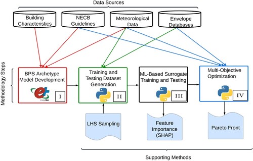
The proposed methodology of this study consists of four main phases, shown in Figure 1 and detailed in the following sub-sections. Phase 1 consists of the base model development, Phase 2 details the dataset generation, which is used in Phase 3 to train and test the surrogate models. The surrogate models are then used in Phase 4 to optimise the possible retrofits of a building.

Figure 1. Methodology flowchart.

2.1. Phase 1 – base model development

An archetype office building is developed using EnergyPlus, following guidelines provided by the National Energy Code of Canada for Buildings (NECB) (Canadian Commission on Building and Fire Codes 2022). As illustrated in Figure 2, the BPS model consists of a three-story building with five zones in each story, including one core zone and four perimeter zones. Table 1 summarises the building’s main characteristics. The accuracy of the model is affirmed through a validation process, where the annual energy use intensity (EUI) is compared with a similar building documented in (Kharvari, Azimi, and O’Brien 2022). The simulated building has an EUI of 105.3 kWh/m², showing less than 5% variance from the EUI reported by Kharvari, Azimi, and O’Brien (2022). This level of difference is deemed acceptable for the purpose of this study.

Figure 2. The archetype BPS model geometry.

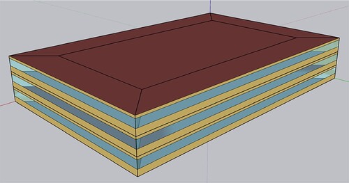
Table 1. Building model initial parameters.

Parameter	Value	Parameter (cnt’d)	Value (cnt’d)
Total floor area (m^2)	4982	Lighting power density (W/m^2)	8.8
Floor area per person	19.92	Plug load density (W/m^2)	10.27
Solar heat gain coefficient (SHGC)	0.31	Boiler efficiency	0.834
Window U-value (W/m^2K)	1.9	Chiller Coefficient of Performance (COP)	4.51
Window-to-wall ratio (WWR) (%)	47.68	Infiltration rate (m^3/s-m^2)	0.00025
Wall U-value (W/m^2K)	0.231	HVAC system	Baseboards connective water heaters and VAV with reheat
Roof U-value (W/m^2K)	0.154	Heating coil fuel	Natural gas
Occupant heat gain (W/person)	130	Chiller type	Scroll electric

2.2. Phase 2- dataset generation

During this stage, a parametric variation of the previously developed BPS model is carried out to generate a dataset encompassing both BPS inputs (features) and outputs (targets). This dataset is then utilised in the subsequent phase for training and testing the ML surrogate models.

As shown in Table 2, the parametric variation included eleven BPS inputs (X1–X11), and three outputs (Y1–Y3), namely annual electricity consumption, peak electric load and Predictive Mean Vote at Standard Effective Temperature (PMVSET). The inputs are selected based on a thorough analysis of previous literature (Pistore et al. 2019; Shen and Pan 2023; Yong et al. 2020; Zhan, He, and Huang 2023), particularly the review conducted by Hashempour, Taherkhani, and Mahdikhani (2020). The PMVSET index is derived from the Pierce comfort model, representing the human body as two concentric compartments: the core responsible for heat generation and the skin (Chen, Yang, and Wang 2017). The model also converts the real environment to a standardised one at SET, which is the dry-bulb temperature of an imaginary environment with 50% relative humidity, where occupants are assumed to be wearing clothing appropriate for the specific activity in the real-world environment. For this metric, values between −1 and 1 are considered comfortable (i.e. when $|\mathrm{PMVSET}|\le 1$), whereas values less than −1 reflect occupants feeling cold, and values greater than 1 reflect occupants feeling warm (Chen, Yang, and Wang 2017).

Table 2. Parameter ranges for training and testing the ML-based surrogate model.

Features/Targets	Range	Reference	Features/Targets	Range	Reference
X1- Wall R-value (m^2K /W)	0.71–10	(Morrison Hershfield 2021)	X8- Cooling Setpoints (time: 6AM – 9PM) (°C)	22.01–26	(Azar and Menassa 2014; Bamdad et al. 2017a; Shen and Pan 2023; Westermann, Welzel, and Evins 2020)
X2- Roof R-value (m^2K /W)	0.53–10	(Morrison Hershfield 2021)	X9- Cooling COP	2.97–5.33	(Love and Bozoian 2022)
X3- Window U-value (W/m^2K)	0.79–6.42	(Love and Bozoian 2022; National Fenestration Rating Council 2023)	X10- Heating efficiency	0.72-0.95	(Love and Bozoian 2022)
X4- SHGC	0–1	(Love and Bozoian 2022; National Fenestration Rating Council 2023)	X11- Infiltration (m^3/s.m^2)	0.000125–0.008	(Chidiac et al. 2011)
X5- Heating Setpoints (time: 9PM – 6AM) (°C)	16–22	(Talami, Dawoodjee, and Ghahramani 2023)	Y1- Electricity (J)	–	–
X6- Heating Setpoints (time: 7AM – 9PM) (°C)	16–22	(Bamdad et al. 2017a; Shen and Pan 2023)	Y2- Peak Load (J)	–	–
X7- Cooling Setpoints (time: 9PM – 6AM) (°C)	22.01–28	(Azar and Menassa 2014; Westermann, Welzel, and Evins 2020)	Y3- PMVSET		–

As for the chosen ranges of the input parameters in Table 2, several databases were used to determine feasible inputs for the surrogate model training and subsequent optimisation. The sources of the values corresponding to these parameters include internal publications by the National Research Council Canada (NRC) (Love and Bozoian 2022), the Building Envelope Thermal Bridging (BETB) guide (Morrison Hershfield 2021), fenestration databases (National Fenestration Rating Council 2023), and other research papers that studied the building stock of Canadian offices (Chidiac et al. 2011). Each of these sources is scanned for suitable values that are code-compliant according to the NECB.

For the surrogate model, continuous ranges between the best and worst values are discretized into 10 intervals to ensure comprehensive coverage of the entire ranges, particularly at the extremes. The parameter ranges are shown in Table 2, which are used for training and testing the ML-based surrogate model. The table also includes the sources from which the ranges are adapted. As detailed later, other discrete values are used during the optimisation stage.

Due to the considerable number of features and their extensive ranges, conducting simulations for all potential scenarios becomes nearly impossible. To overcome this challenge, we employ Latin Hypercube Sampling (LHS), a method that often needs a smaller sample size than random sampling to attain a comparable level of statistical accuracy (Tian et al. 2018). LHS considers each design variable equally important (Choi et al., 2021), ensuring a uniform distribution of samples over the entire range (Ali et al. 2024). The LHS functionality from the Design of Experiments for Python (PyDOE) library is utilised to generate 500 samples, which are later employed in EnergyPlus simulations. In the sampling process, a constraint is implemented on heating and cooling setpoints to guarantee that the heating setpoints consistently remain lower than the cooling setpoints. This precaution is essential to prevent errors that EnergyPlus would otherwise encounter.

The simulation process is automated using the Eppy library, a scripting language designed for EnergyPlus IDF files. Eppy facilitates the data exchange between EnergyPlus and Python, a functionality commonly used in previous studies such as Bui et al. (2021); Ciardiello et al. (2020); Rosso et al. (2020) and Salata et al. (2020). With Eppy, any EnergyPlus object can be effortlessly read and modified, and output files can be processed further (Bui et al. 2020). The simulations are conducted on an hourly basis, resulting in the generation of 8760 data points for each run and a dataset totalling 4,380,000 data points.

Subsequently, the data is further processed and organised into three distinct datasets, each tailored for one target variable. The first dataset contains the sum of hourly electricity consumption for every EnergyPlus run along with the input features, totalling 500 samples. The second dataset encompasses the maximum hourly electricity use (peak load) from each run along with the input features, also totalling 500 samples. The third dataset includes the weather and temporal data, input features, and hourly PMVSET outputs. Notably, weather and temporal data are incorporated into the dataset as crucial determinants in predictive hourly energy models. The weather features include: X12 – Outdoor air temperature (°C); X13 – Relative humidity (%); X14– Wind speed (m/s); X15– Diffuse Radiation (W/m²); and X16– Direct Radiation (W/m²). The temporal features include the day type feature (X17) which differentiates between weekdays and weekends, with values of 0 and 1 assigned to weekends and weekdays respectively, and X18- Hour which represents the hour of the day (from 1 to 24).

2.3. Phase 3 – ML model training and testing

This phase describes the training and testing of ML-based surrogate models using the datasets generated in the previous phase. Several ML models, particularly Linear Regression (LR), Extreme Gradient Boosting (XGB) and Multi-layer Perceptron (MLP), are explored to find the best-fitting model for each target variable. LR, as confirmed by previous studies (Ali et al. 2023; Ciulla and D’Amico 2019), performs reasonably well within a very short time. XGB is recognised as an ensemble learning model with competitive accuracies for building energy performance predictions (Ali et al. 2023; Papadopoulos et al. 2018; Sánchez-Zabala and Gómez-Acebo 2024; Sun, Haghighat, and Fung 2020). XGB is a gradient boosting algorithm that transforms weak learners into strong learners, which, due to its built-in regularisation term, prevents overfitting and controls model complexity, contributing to better predictive performance (Chen et al. 2022). MLP, well-suited for predicting non-linear targets, is a feedforward neural network with a non-linear activation function (Alawi, Kamar, and Yaseen 2024; Chen et al. 2024). Square root target transformation, which helps stabilise variance and makes the target distribution closer to a Gaussian distribution, was also tested as a pre-processing step to help improve the algorithms’ results. The following paragraph details the algorithm chosen for each objective function. When LR performed similarly to XGB and MLP, it was chosen given its simplicity and interpretability.

LR, coupled with a square root target transformation, is used to predict annual electric consumption. As detailed in the subsequent results sections, the model performance achieved satisfactory accuracy levels. XGB, also used with a square root target transformation, is chosen for the peak load predictions. An MLP is employed to predict hourly PMVSET, with min/max scaling applied to the features to ensure all are in the range of 0 to 1. The number of hidden layers in the MLP is set to three, each with 100 neurons, determined by trial and error. The rest of the hyperparameters were set to the values recommended by the used libraries, which include: scikit-learn (Pedregosa et al. 2011) and xgboost (Chen and Guestrin 2016). LinearRegression, TransformedTargetRegressor, MLPRegressor and MinMaxScaler from the scikit-learn library (Pedregosa et al. 2011) and XGB Regressor from the xgboost library (Chen and Guestrin 2016) are the specific methods imported and utilised. All the models are trained on 80% of the data, selected randomly, and tested on the remaining 20%. The final hyperparameter values are summarised in Table 3.

Table 3. Hyperparameter values for each model.

Model	Hyperparameter	Value
XGB	Max_depth: the maximum depth of a tree	6
	Learning_rate: the shrinkage factor controlling the contribution of each tree to the final outcome	0.3
	N_estimators: the number of trees to be generated	100
MLP	Number of hidden layers	3
	Number of hidden layer neurons	100
	Learning_rate: the step size at each iteration	0.001
	Activation: the hidden layer activation function	ReLU
	Solver: the solver for weight optimisation	Adam
	Max_iter: maximum number of iterations	200

The predictive performance of the ML models is assessed using the test set, which constitutes 20% of the datasets. Various error metrics, such as coefficient of determination (R²), mean absolute error (MAE), and coefficient of variation of root mean square error CV(RMSE), are obtained using the equations below. (1) $\begin{array}{rl}{R}^2& =1-\frac{{\mathrm{\Sigma }}_{i=1}^N(y_i-\widehat{y_i})}{{\mathrm{\Sigma }}_{i=1}^N{y}_i-\overline{y_i}}\end{array}$(1) (2) $\begin{array}{rl}\mathrm{Adjusted}{R}^2& =1-\frac{(1-R^2)(N-1)}{N-k-1}\end{array}$(2) (3) $\begin{array}{rl}\mathrm{MAE}& =\frac{{\mathrm{\Sigma }}_{i=1}^N|y_i-\widehat{y_i}|}{N}\end{array}$(3) (4) $\begin{array}{rl}\mathrm{RMSE}& =\sqrt{\left(\frac{{\mathrm{\Sigma }}_{i=1}^N{(y_i-{\hat{y}}_i)}^2}{N}\right)}\end{array}$(4) (5) $\begin{array}{rl}\mathrm{CV}(\mathrm{RMSE})& =\frac{\mathrm{RMSE}}{\frac{1}{N}{\mathrm{\Sigma }}_{i=1}^n{y}_i}\end{array}$(5)

Where $N$ and $k$ correspond to the number of samples and features, and $y_i$, ${\hat{y}}_i$ and ${\overline{y}}_i$ represent the actual, predicted, and mean values, respectively. In this study, both relative (e.g. adjusted R² and CV(RMSE)) and absolute (e.g. MAE) errors are calculated to ensure the model's reliability. Training and testing times are also reported to ensure the computational efficiency of the proposed model.

To gain insights into how the trained model makes predictions, the Shaply additive explanation (SHAP) method is adopted. SHAP is a model-agnostic method, meaning that it can be applied to any ML model (Gugliermetti, Cumo, and Agostinelli 2024). SHAP is one of the most popular interpretation techniques due to its fairness, stability and ability to provide both local and global interpretations (Chen et al. 2023; Gao et al. 2022). Unlike other techniques such as gain and split count (Papadopoulos and Kontokosta 2019), SHAP explains how individual predictions are made by assigning an importance value to individual features, thereby specifying the contribution of each feature to the predicted value based on game theory as shown in Equation (6)(6) $\begin{array}{r}{\varphi }_i={\mathrm{\Sigma }}_{S\subseteq N\{i\}}\left(\frac{|S|!(M-|S|-1)!}{M!}[f_x(S\cup \{i\})-f_x(S)]\right)\end{array}$(6) (Shen and Pan 2023): (6) $\begin{array}{r}{\varphi }_i={\mathrm{\Sigma }}_{S\subseteq N\{i\}}\left(\frac{|S|!(M-|S|-1)!}{M!}[f_x(S\cup \{i\})-f_x(S)]\right)\end{array}$(6) Where N, M, and S are the subset of all input features, the number of input features, and the set of non-zero indexes in $z^{\mathrm{\prime }}$ ($z^{\mathrm{\prime }}\in \{0,1{\}}^M$), respectively. $f_x(S)=E(f(x)|x_S)$ is the model output when the i-th feature is excluded, and $E(f(x)|x_S)$ shows the expected values of the function conditioned on a subset S of the input features. $f_x(S\cup \{i\})$ is the output when the i-th feature is included. This method, however, has two main limitations (Lundberg, Erion, and Lee 2018; Shen and Pan 2023): (1) The calculation of $E(f(x)|x_S)$ is computationally inefficient, and (2) Equation (6) becomes exponentially complex. To address these limitations, the tree SHAP method, best-suited for tree-based models such as XGB, was proposed by Lundberg, Erion, and Lee (2018). The method leverages the structure of decision trees to calculate SHAP values more effectively. It employs a recursive algorithm that traverses the tree, focusing on relevant decision paths, significantly reducing the number of computations compared to the combinatorial approach. The method reduces the computational complexity from O(TL2^M) to O(TLD²), with T, L, and D representing the number of trees, the maximum leaf number, and the tree depth, respectively. The tree SHAP method, however, cannot be used for LR and MLP. For the LR model, LinearExplainer from the SHAP library, tailored for linear models, is used (Lundberg and Lee 2017). This method accounts for feature correlations, thereby preventing collinearity issues and fairly distributing importance among correlated features. Although accounting for correlations can be computationally demanding, LinearExplainer uses sampling to estimate a transformation that can efficiently explain any model prediction. Permutation SHAP is utilised to compute the SHAP values for the MLP model. This method computes SHAP values by iterating through all feature permutations in both forward and reverse directions. Doing this once provides exact SHAP values for models with up to second-order interactions. Repeating this process over many random permutations improves SHAP estimates for models with higher-order interactions.

2.4. Phase 4 – optimization

The validated and tested models from the previous phase are then used to evaluate and optimise possible retrofits for the building along three objective functions, namely, to minimise:

1. Peak load (i.e. the maximum electricity consumed for a single hour of the year).

2. Annual electric load.

3. Thermal discomfort (i.e. the mean absolute value of PMVSET for all occupied hours of the year).

Python’s pymoo is used as the optimisation package due to its large repository of optimisation algorithms (Blank and Deb 2020b). Pymoo has also been shown to work well with black-box optimisation problems that use ML prediction schemes (Biyani 2023). The algorithm class used is ‘genetic algorithms’, as they have been commonly used for similar applications while showing competitive results (e.g. [Costa-Carrapiço, Raslan, and González 2020; Mousavi et al. 2023]). Since this optimisation is a black box problem with three objective functions, the NSGA-II variant of genetic algorithms is deemed suitable (Ma et al. 2023).

The algorithm is set up with a population size of 300 samples, and the duplicates in the initial sample are eliminated and replaced to widen the search space. The algorithm can terminate in 2 different ways. The first is placing a maximum cap of 2000 generations to avoid a comparatively heavy computational load; this is the least desirable termination condition, as the algorithm could terminate before convergence. The other termination condition is a convergence condition measured across a sliding window of 30 generations, which checks for change in the design space (set at 10⁻⁸) and change in the objective space (set at 0.0025) (Blank and Deb 2020a).

For each member of the population, the sampled parameters are used to predict the annual and peak electric loads. For $|\mathrm{PMVSET}|$, the parameters are then duplicated 8760 times (corresponding to the hours of the year) and appended to a data frame that includes the hourly weather data as defined in Phase 2, which is extracted from the required weather file. The weather data is thus not sampled and is kept constant for each member of the population in every generation, since the PMVSET of the building across an entire typical year is being assessed.

The optimisation utilised discrete values for envelope parameters, as shown in Table 4. The two window parameters (U-value and SHGC) are both dependent on the window model chosen, with each U-value corresponding to a specific SHGC value. Thus, the U-value is sampled for each member of the population, and its corresponding SHGC is appended to the data frame, thereby coupling the two parameters. The Window U-values and SHGC values are ordered in the table in accordance with this coupling, and their values are adapted from a database for commercial windows maintained by the National Fenestration Ratings Council (NFRC) (National Fenestration Rating Council 2023). For other values (setpoints, COP, heating efficiency, infiltration), ranges are defined as [min,max,steps], with ‘steps’ specifying how many evenly-spaced values lie between the maximum and minimum (see definition of the ‘linspace’ function in [Oliphant 2015]). These values are based on the existence of a known maximum, minimum, or both (based on the NECB code, for example). Infiltration is a particularly difficult parameter to account for; while existing data was found for air infiltration in other contexts (e.g. [Emmerich and Persily 2014]), the authors could find no similar study for Canadian buildings. Therefore, the initial infiltration condition was assumed to be approximately double the possible minimum.

Table 4. Optimisation parameters.

Parameter	Search space	Parameter (cnt’d)	Search space (cnt’d)
X1: Wall R-value (m^2K/W)	{10, 9.09, 8.33, 7.14, 6.67, 6.25, 5.88, 5.56, 5.26, 5, 4.76, 4.55, 4.39, 4.35, 4.27, 4.22, 4.17} (Morrison Hershfield 2021)	X7: Cooling Setpoint (21:00–6:00)	[min:22, max:26, step:41]
X2: Roof R-value (m^2K/W)	{10, 9.09, 8.33, 7.69} (Morrison Hershfield 2021)	X8: Cooling Setpoint (6:00–21:00)	[min:24, max:28, step:41]
X3: Window U-value (W/m^2K)	{0.79, 0.85, 1.32, 1.44, 1.59, 1.61, 1.69} (Love and Bozoian 2022; National Fenestration Rating Council 2023)	X9: Chiller COP	[min:4.5, max:5.3, step:9]
X4: SHGC	{0.33, 0.33, 0.27, 0.184, 0.3, 0.328, 0.438} (Love and Bozoian 2022; National Fenestration Rating Council 2023)	X10: Heating Efficiency	[min:0.87, max:0.95, step:9]
X5: Heating Setpoint (21:00–6:00)	[min:18, max:22, step:41]	X11: Infiltration (m^3/s/m^2)	[min:0.000125, max:0.0003, step:8]
X6: Heating Setpoint (7:00–21:00)	[min:16, max:20, step:41]

3. Results

This section starts with descriptive data about the performance of the surrogate model, as well as feature importance (Section 3.1). The results of the optimisation are then presented and discussed (Section 3.2).

3.1. ML model evaluation

Table 5 shows the performance metrics of the LR, XGB and MLP models trained to predict annual electric consumption, peak load and hourly PMVSET, respectively. Results indicate high predictive performance for PMVSET, with an adjusted R² value of 0.99 and CV(RMSE) of 0.08, which is well below the 0.3 threshold recommended by ASHRAE Guideline 14 for hourly models. The electricity and peak load targets achieved slightly lower adjusted R² values (0.90 and 0.91, respectively) while still demonstrating a strong predictive capability. The CV(RMSE) values were 0.02 for electricity and 0.03 for peak load, further supporting the reliability of the models in capturing the variability in the data and making predictions. Consequently, the models were deemed valid for use in the subsequent optimisation phase.

Table 5. The performance metrics for the developed models.

Target	Model	Adjusted R^2	MAE	CV(RMSE)	Training and testing time (sec)
Electricity	LR	0.90	7.56 MWh	0.02	0.05
Peak load	XGB	0.91	3.13 kWh	0.03	0.09
PMVSET	MLP	0.99	0.04	0.08	470

The overall training and testing time for the developed model was 0.05 s for the annual electric load surrogate, 0.09 s for the peak load surrogate, and 470 s for the PMVSET surrogate, amounting to about 8 min in total. The training was done using an Intel Core i7-12700H, 2.30 GHz/14 Cores workstation. This time is considered acceptable as the training/testing process is only executed once, and the tested model can be run (for optimisation purposes) instantly.

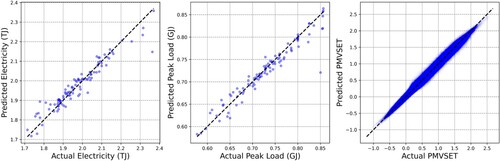
Figure 3 depicts the predicted and actual values for the three targets. In general, the data points are dispersed along the diagonal lines, confirming the strong positive correlation between the predicted and actual values for all three targets. In the cases of electricity and peak load, one instance was notably underestimated for extremely high energy levels. However, this does not compromise the overall accuracy of the models, which was confirmed by the competitive performance metrics described in Table 5. Furthermore, as the models are later used to minimise energy consumption, outliers at the low end of the energy spectrum could have been problematic, and such instances were not observed in the results. As for PMVSET, the points form a tight cluster along the diagonal line, indicating a very strong correlation and high predictive accuracy for the MLP model in predicting hourly PMVSET.

Figure 3. Predicted vs. actual values for electricity, peak load and PMVSET.

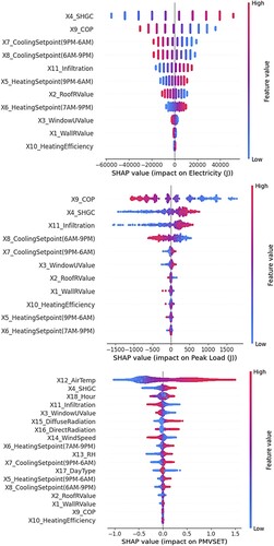
SHAP values are presented in Figure 4. The features are ordered based on the average impact they have on the target variables. In the context of user-defined parameters, SHGC (X4) has a significant impact on electricity consumption, peak load, and PMVSET. Specifically, higher SHGC values correspond to increased electricity usage. This aligns with expectations, as a higher SHGC implies more solar heat gains, subsequently demanding more cooling to maintain a comfortable indoor environment. COP (X9) is another significant factor influencing electricity consumption and peak load, as higher values contribute to lower electricity and peak loads. This relationship is also expected as COP measures the efficiency of the HVAC system. Infiltration (X11) and window U-values (X3) are other influential factors that particularly affect PMVSET, given their contributions to increased heat gains that could cause thermal discomfort. Generally, weather-related and temporal features (e.g. air temperature (X12), direct (X16) and diffuse (X15) radiation and hour of the day (X18)) have significant impacts on PMVSET model outputs, as anticipated. This underscores the importance of relying on hourly-based surrogate models, ensuring a more precise reflection of how weather factors change and affect model outcomes. The impact of building envelope characteristics on performance and the potential implications on retrofit strategies are further discussed in the optimisation results presented next.

Figure 4. Mean SHAP values for the target variables.

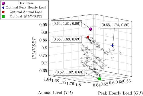
3.2. Optimisation and resulting Pareto front

The optimisation concluded after 334 generations, with 300 nondominated solutions. The 300 solutions are plotted in a 3-dimensional Pareto front, shown in Figure 5. Annual and peak electric loads are generally proportional to the discomfort of the occupants, expressed through high (or non-neutral) PMVSET values. This finding was expected as thermal comfort often requires high energy loads and vice-versa. The Pareto front in Figure 5 shows the three cases with the optimal of each objective function, as well as the base case (simulated on EnergyPlus). The optimal points are significant because even the highlighted solution with the highest $|\mathrm{PMVSET}|$ is well below the comfort limit. The highlighted optimal peak load, annual load, and $|\mathrm{PMVSET}|$ solutions achieved a 14%, 10%, and 34% improvement over their respective base case values. As the archetype office building is code-compliant, relatively small improvements in energy consumption were expected and higher improvements could be achieved had the retrofit measures been applied to an old office building model. The improvement in the $|\mathrm{PMVSET}|$ values, however, is stark, with the optimal peak and annual load solutions recording a 16% and 14% improvement in $|\mathrm{PMVSET}|$, respectively, compared to the base case.

Figure 5. 3D Pareto front with highlighted solutions.

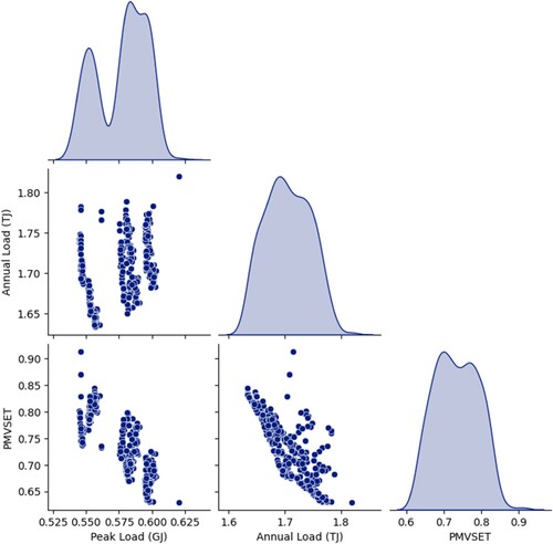
The individual relationship between the three objectives can be further studied by decomposing the 3-dimensional figure into a matrix of 2-dimensional figures, as shown in Figure 6, with the diagonals representing the univariate distribution of each objective within the 300 nondominated solutions. The breakdown in Figure 6 raises several noteworthy observations. Firstly, peak and annual electric loads are weakly correlated to each other, which is contrary to expectation. This could be in part attributed to the clustering of peak loads along a few values that correspond to the maximum loads of different HVAC sizing configurations. Put differently, cooling systems operating at maximum capacity cannot exceed a certain peak load even if higher cooling needs are needed. In contrast, peak and annual electric loads are inversely proportional to $|\mathrm{PMVSET}|$, as expected. For instance, conserving energy (e.g. through higher cooling temperature setpoints) often comes at the expense of indoor thermal conditions and thermal comfort. Secondly, the graphs between the loads and $|\mathrm{PMVSET}|$ show that significant reduction in these loads can be achieved with little increase in $|\mathrm{PMVSET}|$, which is evinced by the large gaps between the cluster of points in the far upper left corner of the two graphs and the points underneath them. The upper left distribution on the diagonal also shows that most solutions found low annual energy consumption values, but that peak values follow a more bimodal distribution, supporting the argument made above on the HVAC system reaching a maximum capacity (and peak load) for different sizing configurations.

Figure 6. Matrix showcasing relationship between individual objectives.

To check the accuracy of the highlighted optimal solutions shown in Figure 5, the input configurations that were used to generate them were extracted and simulated in EnergyPlus. This analysis is done to highlight the accuracy of the surrogate in predicting specific cases that may lie at the boundaries of the search space, since these cases represent the lowest end of the surrogate models’ predictions. More importantly, this analysis helps validate the solutions generated by the proposed ML-based optimisation approach. The differences between the ML-based and EnergyPlus simulations are extracted and shown in Table 6 for each configuration of the objective functions (i.e. optimal peak load, annual load, and |PMVSET|). As shown in the table, all errors are within the ± 3% range, confirming the ability of the surrogate optimisation to find solutions at a high speed and with a relatively low trade-off in accuracy. It is worth noting that the errors are consistently smaller than the improvements reported for the optimal solutions compared to the base case (see Figure 5), reiterating the validity of the results.

Table 6. Error analysis between the surrogate model optimisation solutions and EnergyPlus validation runs.

Optimal configuration	Difference in peak hourly load	Difference in annual load	Difference in |PMVSET|
Opt. peak load	0.06%	−2.12%	0.24%
Opt. annual load	−1.08%	1.78%	2.79%
Opt. |PMVSET|	0.03%	−1.96%	1.74%

The surrogate’s ability to predict PMVSET hourly lends opportunity to further investigate the variation of thermal sensation on an hourly basis across the entire typical year. The inputs resulting in the highlighted values in Figure 5 are extracted and re-simulated to gauge how comfortable the building was throughout occupied hours of the year. These values are not passed through an absolute value function, to help gauge how warm or cold occupants feel throughout the typical year. Results of this analysis are shown in Figure 7, which shows the distribution of values of PMVSET across all occupied hours for the input configurations that returned the optimal of each objective function. Of the four, all boxplots showed a median value between 0 and 1 (where −1 to 1 represents the comfortable range). All three optimal scenarios show that occupants are far more likely to feel warm than cold, which is in line with expectations as natural gas consumption, which is the main heating source, was not considered for this study. It is also worth noting that the median value of all three optimal solutions was lower than that of the base case, further confirming the ability to simultaneously improve energy performance and occupant comfort.

Figure 7. Discomfort boxplot.

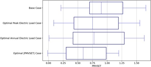
Figure 8 presents the set of inputs that generated the Pareto front distributions shown earlier in Figure 5. Overlaid on the boxplots are the three highlighted solutions and the base case in order to visualise the combinations of inputs that lead to the highlighted solution outputs. Firstly, the inputs related to the building façade showed, for the most part, limited variability in their results, indicating that most solutions share similar optimal values for those parameters. For instance, the optimal window U-value and SHGC combination (X3–4) was (1.44:0.184) for all nondominated solutions, and the roof R-value (X2) tended towards the higher end of the search space for the majority of the solutions. Such values improved all objective functions simultaneously. It can be concluded that passive design strategies for the building envelope are critical for multi-objective performance and were easily identified by the optimisation algorithm. In contrast, the wall R-value (X1) tended towards the lower end of solutions, particularly for the optimal PMVSET scenario. This could be attributed to high insulation levels contributing to the overheating of building spaces (e.g. due to internal heat gains being trapped), hence the model’s converging towards lower R-values to minimise discomfort.

Figure 8. Variation of inputs across the nondominated solution set.

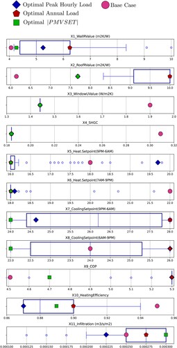
Secondly, operation-related parameters, particularly cooling setpoints, exhibited large variations, partly due to their conflicting impacts on the objective functions (e.g. reducing cooling demand results in suboptimal indoor conditions that increase thermal discomfort). Such parameters are critical for these multi-objective optimizations and should be allocated important time during design to capture synergetic effects and avoid unintended ones. The findings provide ranges that could inform the design of smart building management and control strategies for optimal building performance operation. It is also noteworthy that heating setpoints exhibited little variation, especially during occupied hours. Considering that natural gas was not considered in this study, such parameters would have little effect on energy consumption.

Thirdly, parameters related to the efficiency of the HVAC components (e.g. Heating Efficiency – X10) also showed high variability, which was not necessarily expected. The authors anticipated that the optimisation would converge towards the most energy-efficient values without unintended consequences on occupant comfort. The findings could be attributed to an inverse relationship between the efficiency and needed size (capacity) of the HVAC components. For instance, a high-efficiency boiler might provide the same heating capacity to a building as a larger but less efficient counterpart. System sizing was not controlled in the base case EnergyPlus model, hence the resulting impact on sizing and consequent indoor conditions and comfort levels. The results grant further investigation in future extensions of the current work.

Finally, it is important to reflect on the computational efficiency of the proposed methodology, which was an important motivator for adopting an ML-based BPS surrogate modelling workflow. The optimisation ran for 334 generations, each generation with a population of 300. Considering that the algorithm interacted with the surrogate 8760 times for each hour of the year for $|\mathrm{PMVSET}|$, and twice every year for the electricity metrics, the surrogates were invoked a total of 877,952,400 times. Therefore, it simulated the annual performance of the archetype building 100,200 times, each with different input variations. On an Intel Core i7-12700H, 2.30 GHz/14 Cores workstation, each of these typical years took 21.1 ms to simulate, amounting to a total of approximately 35 min. On the same device, one yearly EnergyPlus simulation of the archetype building required 32 s, meaning that a traditional software-in-the-loop scheme would have required around 38 days. In total, the proposed ML-based surrogate modelling and optimisation approach took 0.08% of the time of a traditional BPS-based workflow, or 1266 times faster. The observed increase in speed is striking and is in agreement with findings by other researchers running comparable experiments (Bamdad et al. 2017b).

4. Conclusion

Recent years have witnessed important research advancements in developing ML-based BPS surrogates to reduce building simulation speeds, as well as optimising building design and retrofit strategies. However, existing efforts have not delved deeply into combining these two areas to harness their capabilities and achieve optimal building solutions at low computational costs. This paper aimed to address these gaps by proposing a unique coupling approach that leverages the capabilities of ML-based surrogate models, utilising a combination of annual and hourly prediction schemes with a multi-objective optimisation algorithm to inform building retrofits along multiple energy and comfort performance metrics. The application of the proposed approach to an archetype office building in Ottawa, ON, Canada, demonstrated and validated its efficacy; optimal design and operation solutions were successfully identified 1266 times faster than a traditional BPS-based optimisation approach.

Despite the stated contributions of the work, it has shortcomings that motivate future research. Firstly, the input database used to explore retrofit strategies could be expanded by gathering building material and construction information from local manufacturers and suppliers. Secondly, additional metrics such as natural gas, CO₂ emissions, and monetary costs were not studied, but they could be added as features in future expansions of the work.

To conclude, this research demonstrated a unique, modular, and scalable approach capable of informing building retrofits at low computational costs. Future steps include further developing the framework's capabilities and working with industrial partners to adapt its content and integrate it into the workflows of practitioners and design professionals.

Acknowledgments

The authors acknowledge the funding support from IC-IMPACTS (India-Canada Centre for Innovative Multidisciplinary Partnerships to Accelerate Community Transformation and Sustainability) and DST (Department of Science and Technology), Government of India, grant number DST/IC/IC-IMPACTS/2022/P-7, as well as the Canada Research Chairs Program. The authors would also like to thank Adam Wills from the National Research Council Canada for providing access to reports that helped improve this work.

Data availability statement

The data that support the findings of this study are available from the corresponding author, E. A., upon reasonable request.

Disclosure statement

No potential conflict of interest was reported by the author(s).

Additional information

Funding

This work was supported by Canada Research Chairs; Department of Science and Technology, Ministry of Science and Technology, India [grant number DST/IC/IC-IMPACTS/2022/P-7]; India-Canada Centre for Innovative Multidisciplinary Partnerships to Accelerate Community Transformation and Sustainability (IC-IMPACTS) [grant number DST/IC/IC-IMPACTS/2022/P-7].

References

- Alawi, O. A., H. M. Kamar, and Z. M. Yaseen. 2024. “Optimizing Building Energy Performance Predictions: A Comparative Study of Artificial Intelligence Models.” Journal of Building Engineering 88:109247. https://doi.org/10.1016/j.jobe.2024.109247.
- Ali, U., S. Bano, M. H. Shamsi, D. Sood, C. Hoare, W. Zuo, N. Hewitt, and J. O’Donnell. 2024. “Urban Building Energy Performance Prediction and Retrofit Analysis Using Data-Driven Machine Learning Approach.” Energy and Buildings 303:113768. https://doi.org/10.1016/j.enbuild.2023.113768.
- Ali, A., R. Jayaraman, A. Mayyas, B. Alaifan, and E. Azar. 2023. “Machine Learning as a Surrogate to Building Performance Simulation: Predicting Energy Consumption Under Different Operational Settings.” Energy and Buildings 286:112940. https://doi.org/10.1016/j.enbuild.2023.112940.
- Azar, E., and C. C. Menassa. 2014. “A Comprehensive Framework to Quantify Energy Savings Potential from Improved Operations of Commercial Building Stocks.” Energy Policy 67:459–472. https://doi.org/10.1016/j.enpol.2013.12.031.
- Bamdad, K., M. E. Cholette, and J. Bell. 2020. “Building Energy Optimization Using Surrogate Model and Active Sampling.” Journal of Building Performance Simulation 13 (6): 760–776. https://doi.org/10.1080/19401493.2020.1821094.
- Bamdad, K., M. E. Cholette, L. Guan, and J. Bell. 2017a. “Ant Colony Algorithm for Building Energy Optimisation Problems and Comparison with Benchmark Algorithms.” Energy and Buildings 154:404–414. https://doi.org/10.1016/j.enbuild.2017.08.071.
- Bamdad, K., M. Cholette, L. Guan, and J. Bell. 2017b. “Building Energy Optimisation Using Artificial Neural Network and Ant Colony Optimisation.” In Proceedings of the Australasian Building Simulation Conference 2017, edited by P. Bannister, 1–11. Melbourne, Australia: The Australian Institute of Refrigeration, Air Conditioning and Heating (AIRAH).
- Bell, N. 2023. The Path to Zero Energy Office Buildings – Energy retrofitting of commercial office buildings [UNSW Sydney]. https://doi.org/10.26190/UNSWORKS/25029.
- Biyani, P. 2023. “Solving Multi-Objective Constrained Optimisation Problems using Pymoo.” EuroPython, July 17. https://ep2023.europython.eu/session/solving-multi-objective-constrained-optimisation-problems-using-pymoo/.
- Blank, J., and K. Deb. 2020a. “A Running Performance Metric and Termination Criterion for Evaluating Evolutionary Multi- and Many-Objective Optimization Algorithms.” 2020 IEEE Congress on Evolutionary Computation (CEC), 1–8. https://doi.org/10.1109/CEC48606.2020.9185546.
- Blank, J., and K. Deb. 2020b. “Pymoo: Multi-Objective Optimization in Python.” IEEE Access 8:89497–89509. https://doi.org/10.1109/ACCESS.2020.2990567.
- Bui, D.-K., T. N. Nguyen, A. Ghazlan, and T. D. Ngo. 2021. “Biomimetic Adaptive Electrochromic Windows for Enhancing Building Energy Efficiency.” Applied Energy 300:117341. https://doi.org/10.1016/j.apenergy.2021.117341.
- Bui, D.-K., T. N. Nguyen, A. Ghazlan, N.-T. Ngo, and T. D. Ngo. 2020. “Enhancing Building Energy Efficiency by Adaptive Façade: A Computational Optimization Approach.” Applied Energy 265:114797. https://doi.org/10.1016/j.apenergy.2020.114797.
- Canadian Commission on Building and Fire Codes. 2022. National Energy Code of Canada for Buildings: 2020. 317 p. https://doi.org/10.4224/RR3Q-HM83.
- Chen, Z., Y. Cui, H. Zheng, and Q. Ning. 2024. “Optimization and Prediction of Energy Consumption, Light and Thermal Comfort in Teaching Building Atriums Using NSGA-II and Machine Learning.” Journal of Building Engineering 86:108687. https://doi.org/10.1016/j.jobe.2024.108687.
- Chen, T., and C. Guestrin. 2016. “XGBoost: A Scalable Tree Boosting System.” Proceedings of the 22nd ACM SIGKDD International Conference on Knowledge Discovery and Data Mining, 785–794. https://doi.org/10.1145/2939672.2939785.
- Chen, Y., M. Guo, Z. Chen, Z. Chen, and Y. Ji. 2022. “Physical Energy and Data-Driven Models in Building Energy Prediction: A Review.” Energy Reports 8:2656–2671. https://doi.org/10.1016/j.egyr.2022.01.162.
- Chen, Z., F. Xiao, F. Guo, and J. Yan. 2023. “Interpretable Machine Learning for Building Energy Management: A State-of-the-Art Review.” Advances in Applied Energy 9:100123. https://doi.org/10.1016/j.adapen.2023.100123.
- Chen, X., H. Yang, and Y. Wang. 2017. “Parametric Study of Passive Design Strategies for High-Rise Residential Buildings in Hot and Humid Climates: Miscellaneous Impact Factors.” Renewable and Sustainable Energy Reviews 69:442–460. https://doi.org/10.1016/j.rser.2016.11.055.
- Chidiac, S. E., E. J. C. Catania, E. Morofsky, and S. Foo. 2011. “A Screening Methodology for Implementing Cost Effective Energy Retrofit Measures in Canadian Office Buildings.” Energy and Buildings 43 (2-3): 614–620. https://doi.org/10.1016/j.enbuild.2010.11.002.
- Choi, Y., D. Song, S. Yoon, and J. Koo. 2021. “Comparison of Factorial and Latin Hypercube Sampling Designs for Meta-Models of Building Heating and Cooling Loads.” Energies 14 (2): Article 2. https://doi.org/10.3390/en14020512.
- Ciardiello, A., F. Rosso, J. Dell’Olmo, V. Ciancio, M. Ferrero, and F. Salata. 2020. “Multi-Objective Approach to the Optimization of Shape and Envelope in Building Energy Design.” Applied Energy 280:115984. https://doi.org/10.1016/j.apenergy.2020.115984.
- Ciulla, G., and A. D’Amico. 2019. “Building Energy Performance Forecasting: A Multiple Linear Regression Approach.” Applied Energy 253:113500. https://doi.org/10.1016/j.apenergy.2019.113500.
- Costa-Carrapiço, I., R. Raslan, and J. N. González. 2020. “A Systematic Review of Genetic Algorithm-Based Multi-Objective Optimisation for Building Retrofitting Strategies Towards Energy Efficiency.” Energy and Buildings 210:109690. https://doi.org/10.1016/j.enbuild.2019.109690.
- Daly, D., P. Cooper, and Z. Ma. 2018. “Qualitative Analysis of the Use of Building Performance Simulation for Retrofitting Lower Quality Office Buildings in Australia.” Energy and Buildings 181:84–94. https://doi.org/10.1016/j.enbuild.2018.09.040.
- Emmerich, S. J., and A. K. Persily. 2014. “Analysis of U.S. Commercial Building Envelope Air Leakage Database to Support Sustainable Building Design.” International Journal of Ventilation 12 (4): 331–344. https://doi.org/10.1080/14733315.2014.11684027.
- Evins, R. 2013. “A Review of Computational Optimisation Methods Applied to Sustainable Building Design.” Renewable and Sustainable Energy Reviews 22:230–245. https://doi.org/10.1016/j.rser.2013.02.004.
- Gao, Y., H. Han, H. Lu, S. Jiang, Y. Zhang, and M. Luo. 2022. “Knowledge Mining for Chiller Faults Based on Explanation of Data-Driven Diagnosis.” Applied Thermal Engineering 205:118032. https://doi.org/10.1016/j.applthermaleng.2021.118032.
- Gugliermetti, L., F. Cumo, and S. Agostinelli. 2024. “A Future Direction of Machine Learning for Building Energy Management: Interpretable Models.” Energies 17 (3): Article 3. https://doi.org/10.3390/en17030700.
- Hashempour, N., R. Taherkhani, and M. Mahdikhani. 2020. “Energy Performance Optimization of Existing Buildings: A Literature Review.” Sustainable Cities and Society 54:101967. https://doi.org/10.1016/j.scs.2019.101967.
- Kharvari, F., S. Azimi, and W. O’Brien. 2022. “A Comprehensive Simulation-Based Assessment of Office Building Performance Adaptability to Teleworking Scenarios in Different Canadian Climate Zones.” Building Simulation 15 (6): 995–1014. https://doi.org/10.1007/s12273-021-0864-x.
- Li, G., W. Tian, H. Zhang, and X. Fu. 2023. “A Novel Method of Creating Machine Learning-Based Time Series Meta-Models for Building Energy Analysis.” Energy and Buildings 281:112752. https://doi.org/10.1016/j.enbuild.2022.112752.
- Li, X., and J. Wen. 2014. “Review of Building Energy Modeling for Control and Operation.” Renewable and Sustainable Energy Reviews 37:517–537. https://doi.org/10.1016/j.rser.2014.05.056.
- Love, C., and S. Bozoian. 2022. Defining Energy Efficiency Measures and Their Impacts. Victoria, BC, Canada: RDH Building Science.
- Lundberg, S. M., G. G. Erion, and S.-I. Lee. 2018. “Consistent Individualized Feature Attribution for Tree Ensembles.” arXiv Preprint arXiv:1802.03888.
- Lundberg, S. M., and S.-I. Lee. 2017. “A Unified Approach to Interpreting Model Predictions.” Advances in Neural Information Processing Systems 30. https://proceedings.neurips.cc/paper/2017/hash/8a20a8621978632d76c43dfd28b67767-Abstract.html.
- Ma, H., Y. Zhang, S. Sun, T. Liu, and Y. Shan. 2023. “A Comprehensive Survey on NSGA-II for Multi-Objective Optimization and Applications.” Artificial Intelligence Review 56 (12): 15217–15270. https://doi.org/10.1007/s10462-023-10526-z.
- Mariano-Hernández, D., L. Hernández-Callejo, A. Zorita-Lamadrid, O. Duque-Pérez, and F. Santos García. 2021. “A Review of Strategies for Building Energy Management System: Model Predictive Control, Demand Side Management, Optimization, and Fault Detect & Diagnosis.” Journal of Building Engineering 33:101692. https://doi.org/10.1016/j.jobe.2020.101692.
- Morrison Hershfield. 2021. Building Envelope Thermal Bridging Guide. https://www.bchydro.com/content/dam/BCHydro/customer-portal/documents/power-smart/builders-developers/building-envelope-thermal-bridging-guide-v1-6.pdf.
- Mousavi, S., M. G. Villarreal-Marroquín, M. Hajiaghaei-Keshteli, and N. R. Smith. 2023. “Data-driven Prediction and Optimization Toward net-Zero and Positive-Energy Buildings: A Systematic Review.” Building and Environment 242:110578. https://doi.org/10.1016/j.buildenv.2023.110578.
- National Fenestration Rating Council. 2023. NFRC Certified Products Directory for Non-Residential Fenestration Energy Certification and Rating [dataset]. https://cmast.nfrc.org/?AspxAutoDetectCookieSupport=1.
- National Research Council Canada. 2020. Final Report—Alterations to Existing Buildings. Government of Canada.
- Natural Research Council Canada. 2018. Major Energy Retrofit Guidelines for Commercial and Institutional Buildings: Office Buildings. Ottawa, ON, Canada: Natural Resources Canada.
- Natural Resources Canada. 2022. The Canada Green Buildings Strategy [Discussion Paper]. Government of Canada. https://natural-resources.canada.ca/sites/nrcan/files/public-consultation/cgbs-discussion-paper-2023-08-03-eng.pdf.
- Oliphant, T. E. 2015. Guide to NumPy. 2nd ed. Scotts Valley, CA: Continuum Press, a division of Continuum Analytics, Inc.
- Papadopoulos, S., E. Azar, W.-L. Woon, and C. E. Kontokosta. 2018. “Evaluation of Tree-Based Ensemble Learning Algorithms for Building Energy Performance Estimation.” Journal of Building Performance Simulation 11 (3): 322–332. https://doi.org/10.1080/19401493.2017.1354919.
- Papadopoulos, S., and C. E. Kontokosta. 2019. “Grading Buildings on Energy Performance Using City Benchmarking Data.” Applied Energy 233-234:244–253. https://doi.org/10.1016/j.apenergy.2018.10.053.
- Pedregosa, F., G. Varoquaux, A. Gramfort, V. Michel, B. Thirion, O. Grisel, M. Blondel, et al. 2011. “Scikit-Learn: Machine Learning in Python.” Journal of Machine Learning Research 12 (85): 2825–2830.
- Pistore, L., G. Pernigotto, F. Cappelletti, A. Gasparella, and P. Romagnoni. 2019. “A Stepwise Approach Integrating Feature Selection, Regression Techniques and Cluster Analysis to Identify Primary Retrofit Interventions on Large Stocks of Buildings.” Sustainable Cities and Society 47:101438. https://doi.org/10.1016/j.scs.2019.101438.
- Qian, Z., C. C. Seepersad, V. R. Joseph, J. K. Allen, and C. F. Jeff Wu. 2005. “Building Surrogate Models Based on Detailed and Approximate Simulations.” Journal of Mechanical Design 128 (4): 668–677. https://doi.org/10.1115/1.2179459.
- Rabani, M., H. B. Madessa, and N. Nord. 2017. “A State-of-Art Review of Retrofit Interventions in Buildings Towards Nearly Zero Energy Level.” Energy Procedia 134:317–326. https://doi.org/10.1016/j.egypro.2017.09.534.
- Rosso, F., V. Ciancio, J. Dell’Olmo, and F. Salata. 2020. “Multi-Objective Optimization of Building Retrofit in the Mediterranean Climate by Means of Genetic Algorithm Application.” Energy and Buildings 216:109945. https://doi.org/10.1016/j.enbuild.2020.109945.
- Salata, F., V. Ciancio, J. Dell’Olmo, I. Golasi, O. Palusci, and M. Coppi. 2020. “Effects of Local Conditions on the Multi-Variable and Multi-Objective Energy Optimization of Residential Buildings Using Genetic Algorithms.” Applied Energy 260:114289. https://doi.org/10.1016/j.apenergy.2019.114289.
- Sánchez-Zabala, V. F., and T. Gómez-Acebo. 2024. “Building Energy Performance Metamodels for District Energy Management Optimisation Platforms.” Energy Conversion and Management: X 21:100512. https://doi.org/10.1016/j.ecmx.2023.100512.
- Shaikh, P. H., N. B. M. Nor, P. Nallagownden, I. Elamvazuthi, and T. Ibrahim. 2014. “A Review on Optimized Control Systems for Building Energy and Comfort Management of Smart Sustainable Buildings.” Renewable and Sustainable Energy Reviews 34:409–429. https://doi.org/10.1016/j.rser.2014.03.027.
- Shen, Y., and Y. Pan. 2023. “BIM-supported Automatic Energy Performance Analysis for Green Building Design Using Explainable Machine Learning and Multi-Objective Optimization.” Applied Energy 333:120575. https://doi.org/10.1016/j.apenergy.2022.120575.
- Sun, Y., F. Haghighat, and B. C. M. Fung. 2020. “A Review of the-State-of-the-art in Data-Driven Approaches for Building Energy Prediction.” Energy and Buildings 221:110022. https://doi.org/10.1016/j.enbuild.2020.110022.
- Talami, R., I. Dawoodjee, and A. Ghahramani. 2023. “Quantifying Energy Savings from Optimal Selection of HVAC Temperature Setpoints and Setbacks Across Diverse Occupancy Rates and Patterns.” Buildings 13 (12): Article 12. https://doi.org/10.3390/buildings13122998.
- Tian, W., Y. Heo, P. de Wilde, Z. Li, D. Yan, C. S. Park, X. Feng, and G. Augenbroe. 2018. “A Review of Uncertainty Analysis in Building Energy Assessment.” Renewable and Sustainable Energy Reviews 93:285–301. https://doi.org/10.1016/j.rser.2018.05.029.
- Tresidder, E., Y. Zhang, and A. I. J. Forrester. 2011. “Optimisation of Low-Energy Building Design Using Surrogate Models.” Proceedings of Building Simulation 2011. 12th Conference of International Building Performance Simulation Association.
- Tresidder, E., Y. Zhang, and A. I. J. Forrester. 2012. “Acceleration of Building Design Optimisation Through the Use of Kriging Surrogate Models.” In Proceedings of Building Simulation and Optimization. First Building Simulation and Optimization Conference. 1–8. Loughborough, UK.
- Westermann, P., and R. Evins. 2019. “Surrogate Modelling for Sustainable Building Design – A Review.” Energy and Buildings 198:170–186. https://doi.org/10.1016/j.enbuild.2019.05.057.
- Westermann, P., M. Welzel, and R. Evins. 2020. “Using a Deep Temporal Convolutional Network as a Building Energy Surrogate Model That Spans Multiple Climate Zones.” Applied Energy 278:115563. https://doi.org/10.1016/j.apenergy.2020.115563.
- Yang, H., and C. Liu. 2018. “Multi-Objective Optimization Design Approach for Green Building Retrofit Based on BIM and BPS in the Cold Region of China.” In eWork and Ebusiness in Architecture, Engineering and Construction: Proceedings of the 12th European Conference on Product and Process Modelling (ECPPM 2018), edited by J. Karlshøj and R. J. Scherer, 87–94. Copenhagen, Denmark: CRC Press.
- Yong, Z., Y. Li-juan, Z. Qian, and S. Xiao-yan. 2020. “Multi-Objective Optimization of Building Energy Performance Using a Particle Swarm Optimizer with Less Control Parameters.” Journal of Building Engineering 32:101505. https://doi.org/10.1016/j.jobe.2020.101505.
- Zhan, J., W. He, and J. Huang. 2023. “Dual-Objective Building Retrofit Optimization Under Competing Priorities Using Artificial Neural Network.” Journal of Building Engineering 70:106376. https://doi.org/10.1016/j.jobe.2023.106376.