Juvenile Steelhead Distribution, Migration, Feeding, and Growth in the Columbia River Estuary, Plume, and Coastal Waters

Abstract

Relative to extensive research on the freshwater stages of steelhead Oncorhynchus mykiss life history, little is known about the species’ estuarine and early marine phases despite the decline of numerous populations, including several from the Columbia River. Comparisons of the distribution, diet, and growth of juvenile steelhead collected during surveys of the Columbia River estuary and coastal waters in May, June, and September 1998–2011 were analyzed for comparisons between fish caught in the estuary and ocean and between hatchery (marked) and putative wild (unmarked) fish. Almost all catches of juvenile steelhead in the ocean occurred during the May surveys (96%). Juvenile steelhead were consistently caught at the westernmost stations (>55 km from shore), indicating an offshore distribution. Based on otolith structure and chemistry, we determined that these juveniles had been in marine waters for an average of only 9.8 d (SD = 10.2). Some of the steelhead that had been in marine waters for 1–3 d were captured at the westernmost edge of survey transects, indicating rapid offshore migration. Estuary-caught fish ate fewer prey types and consumed far less food than did ocean-caught fish, which ate a variety of prey, including juvenile fishes, euphausiids, and crab megalopae. Estuary- and ocean-caught unmarked fish exhibited higher feeding intensities, fewer empty stomachs, and better condition than hatchery fish. Growth hormone levels (insulin-like growth factor 1 [IGF-1]) in unmarked fish and hatchery fish varied annually, with unmarked fish having slightly higher overall values. In general, the FL, condition, stomach fullness, and IGF-1 of ocean-caught steelhead increased with distance offshore. Unlike juveniles of other salmonid species, steelhead appeared to quickly migrate westward from coastal rivers and showed patterns of increased feeding and growth in offshore waters. An understanding of the estuarine and ocean ecology of steelhead smolts may assist in the management of threatened steelhead populations.

Received July 18, 2013; accepted November 21, 2013

Anadromous salmonids initially spend the earliest stages of their life history in freshwater, migrate through estuarine systems as juvenile-stage smolts, and then enter marine waters for increased feeding and growth opportunities. After a marine residency period of several months to years, during which they accrue the majority of their adult biomass, the salmon return to freshwater to spawn. Salmonid residence time in each habitat is highly variable and dependent upon the species and population (Quinn and Myers 2004); the variation in productivity in different climate regimes influences, in part, these differences in reliance on freshwater and marine habitats. Consequently, the factors that affect foraging success and predator avoidance during the transition to marine environments may influence the dynamics of salmonid populations.

Populations of steelhead Oncorhynchus mykiss (anadromous Rainbow Trout) are widely distributed along the Pacific coast of North America and extend to the Kamchatka Peninsula in Russia (Augerot 2005). Steelhead have one of the most diverse life histories within the genus Oncorhynchus (Quinn 2005). The life history strategy of steelhead is most similar to that of sea-run Atlantic Salmon Salmo salar. Both species remain in rivers as young for 1–4 years, migrate to sea in the spring, spend variable numbers of years in open-ocean waters, and return to their natal rivers to spawn; subsequently, they may return to the ocean and back to freshwater to spawn several more times. There are also extensive similarities between the freshwater residency of anadromous Cutthroat Trout O. clarkii and that of steelhead, yet the two species have vastly different marine life histories. After leaving freshwater, Cutthroat Trout typically remain in coastal waters and return to spawn after a short marine duration, whereas steelhead remain at sea longer and migrate farther (Pearcy et al. 1990; Moore et al. 2010b).

The National Oceanic and Atmospheric Administration (NOAA) has identified 15 distinct population segments of steelhead in Oregon, Washington, Idaho, and California based on genetics, phylogeny and life history, and freshwater ichthyogeography (Busby et al. 1996). Of these distinct population segments, 11 are currently listed as threatened or endangered under the U.S. Endangered Species Act (ESA). Despite these ESA listings and extensive research on freshwater residency, there has been little research on the estuarine and early marine phases of steelhead life history. Marine mortality of juvenile salmon is high (Quinn 2005), with the highest levels thought to occur early in the marine phase (Pearcy 1992). Additionally, millions of hatchery salmon are produced annually, but research on differences between hatchery- and naturally produced salmon in the marine and estuarine environments has been relatively scarce (Chittenden et al. 2008; Daly et al. 2011; Beamish et al. 2012).

Columbia River steelhead juveniles migrate to the ocean in mid-April through early June, with peak migration typically occurring in mid-May (Weitkamp et al. 2012). Juvenile steelhead feed at low rates while migrating through the estuary (Dawley et al. 1986). Acoustic telemetry data suggest that Puget Sound steelhead also migrate quickly through coastal estuaries (Moore et al. 2010a) unlike other Pacific salmon, which reside in the estuarine environment for longer periods of time (Quinn 2005). In coastal California rivers, the larger steelhead smolts migrate quickly through estuaries, whereas the smaller steelhead smolts exhibit longer estuarine residency, allowing them to double in size before migrating offshore (Bond et al. 2008). It is believed that once the juvenile steelhead enter coastal waters, they move quickly offshore to oceanic feeding grounds, bypassing the coastal migration routes used by other anadromous Pacific salmonids (Burgner et al. 1992; Augerot 2005). Information on the coastal distribution of steelhead shortly after ocean entry was obtained via purse-seine surveys conducted during the 1960s from north of Washington to Alaska (Hartt and Dell 1986) and during the 1980s in coastal waters off Oregon and Washington (Miller et al. 1983; Pearcy and Fisher 1990; Pearcy et al. 1990). In addition to the purse-seine surveys, high-seas tagging data suggest that age-1 steelhead are located farther offshore (average distance = 2,257 km) than other juvenile salmonids, with only age-1 Chum Salmon O. keta migrating distances even close to those of steelhead (1,918 km; Quinn and Myers 2004).

The objective of this work was to analyze the distribution, diet, condition, and growth of juvenile steelhead in the Columbia River estuary and during early marine residence. We summarized 14 years of ocean surveys (1998–2011) and 4 years of estuary surveys (2008–2011) and examined the hypothesis that juvenile steelhead in the marine environment and juveniles in the Columbia River estuary are similar in size and condition and have comparable levels of stomach fullness. We also hypothesized that hatchery and wild fish would be indistinguishable from each other based on diet, growth, and condition; if so, these metrics in hatchery steelhead could be used as proxies for those in putative wild (unmarked) steelhead. We analyzed annual changes in ocean abundance, diet (diet composition and stomach fullness), size, growth, and condition and considered whether variations in these biological metrics were related. Finally, we determined the average length of marine residence in coastal waters and evaluated whether there were identifiable changes in biological metrics as steelhead migrated to shelf waters. These data will fill gaps in knowledge of this transitional phase of steelhead life history and may provide valuable information for management decisions aimed at improving ESA-listed steelhead populations.

METHODS

Sample collection.—Data describing juvenile steelhead were collected from two ongoing studies: (1) Columbia River estuary data were from a study directed toward the spring out-migration period of juvenile salmonids as they moved through the estuary just before marine entry, and (2) marine data were from NOAA Fisheries’ pelagic trawl surveys that targeted the early marine phase of juvenile salmonids off the coasts of Washington and Oregon. The estuarine data were analyzed to assess the biological condition of smolts (i.e., size, condition, and general feeding habits) before entry into the marine environment. Ocean survey data included steelhead size and condition as well as more extensive diet analysis, migration patterns (site of origin to location of capture), growth, and timing of marine entry.

Pelagic ocean surveys occurred in May (1999–2011), June (1998–2011), and September (1998–2011). Samples were collected at three to nine transects, each with five to seven predetermined sampling stations, extending from inshore to near the continental shelf break. Limited May surveys during 2000–2005 included only three transects: one off the Columbia River mouth (46.2°N), one north of the river, and one south of the river. With few exceptions, other May survey years and all June and September surveys were conducted from Newport, Oregon (44.6°N), to an area near the mouth of the Strait of Juan de Fuca, Washington (48.2°N).

Fish were collected with a Nordic 264 pelagic rope trawl, which had a 30-m-wide × 20-m-deep mouth opening and was fitted with a 0.8-cm cod-end liner. The rope trawl was towed for 30 min during daylight at approximately 6 km/h, with the headrope within 1 m of the surface (Brodeur et al. 2005). All captured salmonids were identified to species, measured (FL, nearest 1 mm), individually labeled, and immediately frozen. Prior to freezing, each fish was also checked for an adipose fin clip, which if present would indicate hatchery origin.

In addition to the regular surveys described above, sites around the Columbia River's freshwater plume front were sampled during a special study in late May of 2001 and 2002 (De Robertis et al. 2005). These fish were collected slightly north of the Columbia River transect between 11 and 40 km offshore, and their migration patterns and diet composition information were included in our data sets. We collected one additional coded-wire-tagged fish during another special study conducted near the Columbia River mouth in May 2004, and this fish was included in our tagging data set.

Estuary collections of juvenile steelhead occurred from 2007 to 2011 at two stations in the lower Columbia River estuary: North Channel (46°14.2′N, 123°54.2′W; river kilometer [rkm] 17) and Trestle Bay (46°12.9′N, 123°57.7′W; rkm 13; see Weitkamp et al. 2012 for further details). Sampling was restricted to days with early morning low tides, which typically occur during extreme (minus) tides in spring. The first set was made at approximately low slack water, and sampling continued for the duration of the flood tide. Fish were sampled with a fine-mesh purse seine (10.6 m deep × 155 m long; stretched mesh opening = 1.7 cm; knotless bunt mesh = 1.5 cm). We restricted sampling to a depth of 8–10 m in order to sample the entire water column. All captured steelhead were anaesthetized; checked for the presence of a coded wire tag (CWT), PIT tag, or adipose fin clip; and measured to the nearest 1 mm (CWTs are commonly inserted into hatchery fish to mark those fish with information on their hatchery of origin and release data; PIT tags are commonly inserted into hatchery fish, and to a lesser degree naturally produced fish, to track individuals through time). A subset of juvenile steelhead was retained for laboratory analysis (no fish were retained in 2007) and given a lethal dose of tricaine methanesulfonate (MS-222) before being individually tagged, bagged, and frozen. Juvenile steelhead that were not needed for laboratory analyses were allowed to fully recover and then were released.

In the laboratory, field identification of estuary- and ocean-caught salmonids was verified, and each fish was re-measured (FL, nearest 1 mm), weighed (nearest 0.1 g), and rechecked for any markings or tags (clipped adipose fin, CWT, PIT tag, or latex tag [another, less commonly used hatchery tag]). Stomachs were removed and placed in a 10% formaldehyde solution for approximately 2 weeks; they were then rinsed with freshwater for 24 h before being transferred into a 70% solution of ethanol. Because some shrinkage occurs after fish have been frozen, we used FL measurements taken in the field for all analyses.

Table 1 Numbers of juvenile steelhead that were sampled in marine waters off the coasts of Oregon and Washington during annual May surveys. Counts of steelhead were adjusted by the annual rate of hatchery marking to estimate the numbers of unmarked fish and hatchery fish.

Year	Hatchery marking rate (%)	Adjusted number of naturally produced fish	Adjusted number of hatchery fish	Total number of fish sampled
2000	82.0	5	2	7^a
2001	73.0	23	79	102^a
2002	79.2	21	75	96^a
2003	79.5	2	1	3^a
2004	80.5	3	30	33^a
2005	86.0	0	0	0^a
2006	82.7	45	247	292^a
2007	83.9	23	22	45^a
2008	80.4	26	48	74^a
2009	79.8	11	32	43^a
2010	82.1	16	30	46^a
2011	87.8	14	25	39^a

^aIncludes special study fish that were collected in May of 2001 and 2002 (De Robertis et al. 2005).

Captured steelhead consisted of both hatchery fish and unmarked fish. Most hatchery fish are marked with a fin clip or tag to distinguish them from natural-origin or “wild” fish. If a tag or adipose fin clip was present, the fish was considered to be of hatchery origin unless the PIT tag identified the fish as being of natural origin. Hatchery-produced steelhead (hereafter, “hatchery steelhead”) sampled in our study would have originated primarily from the Columbia River basin, where approximately 15 million (SD = 0.9 million) hatchery fish are released each year. These include 4.0 million (SD = 0.6 million) from the lower Columbia River, 9.0 million (SD = 0.9 million) from the Snake River, and 2.1 million (SD = 0.4 million) from the upper and middle Columbia River. Other potential sources of hatchery steelhead in our samples were coastal Oregon rivers, where 2.0 million (SD = 0.2 million) juvenile steelhead are released annually, and coastal Washington rivers, where 2.2 million (SD = 0.3 million) are released each year.

The average marking rate for hatchery steelhead in the Columbia River basin is 84.5% (SD = 4.0%); coastal Oregon hatcheries have a slightly higher marking rate at 90.5% (SD = 3.7%), and coastal Washington hatcheries mark at a lower rate of 55.8% (SD = 11.6%). Data on hatchery releases and marking rates were obtained from the Regional Mark Information System database (Regional Mark Processing Center, www.rmpc.org, accessed November 2012). Hatchery steelhead releases and marking rates used for analyses were averages from the years encompassing our ocean surveys.

Because hatchery marking rates were less than 100%, unmarked steelhead represented a mixture of both naturally produced and hatchery individuals, and the origin of individual unmarked fish could not be determined with certainty. To calculate the potential number of naturally produced (putative wild) steelhead caught for each survey, we divided the percentage of the catch that were hatchery-marked fish by the percentage of adipose-fin-clipped fish released from hatcheries in that same year (Table 1). This adjusted percent hatchery of the catch was used to remove a predicted number of the unmarked fish that were potentially of hatchery origin and to estimate the number of naturally produced fish in a given year. For our biological comparisons between marked and unmarked fish (described below), biological data from some unmarked hatchery fish were likely included with data from natural-origin fish. This inclusion could blur biological differences between the two populations; therefore, results of comparisons between unmarked and marked fish should be considered conservative.

Distribution, origin, and migration.—The ocean distribution of juvenile steelhead was determined by calculating the CPUE, defined as the number of fish per kilometer towed at each station. We calculated an average CPUE of hatchery and unmarked fish per station from May surveys during years when the full grid of transects was sampled (1999 and 2006–2011). Only 24 juvenile steelhead were captured during our June surveys, but we also calculated the average CPUE per station for June 1998–2011. For September surveys, juvenile steelhead distribution was not calculated due to extremely limited catch data (n = 1 fish). No further analyses were conducted for the June or September survey data. We mapped the annual May distributions of ocean-caught steelhead.

The Columbia River plume is the surface layer of lower-salinity Columbia River water that extends into the Pacific Ocean. The size and location of the plume are affected primarily by river discharge and ocean wind patterns (Burla et al. 2010b). Salinity was measured at each sampling station by using a Sea-Bird SBE-19plus conductivity–temperature–depth recorder (Sea-Bird Electronics, Bellevue, Washington). The CPUE was log(x + 0.1) transformed, and differences in CPUE between plume waters (salinity < 28‰ at 1-m depth) and non-plume waters (salinity > 28‰) were evaluated with the Mann–Whitney W-test (α = 0.05). We used the salinity threshold for plume waters as defined by Burla et al. (2010b).

Coded wire tags or PIT tags from ocean-caught juvenile steelhead were examined to obtain information about release location and timing and geographic origin. For fish containing CWTs or PIT tags, we extracted the tags, “read” the tag code visually (CWTs) or electronically (PIT tags), and determined the release location and date from online databases (CWTs: Regional Mark Processing Center, www.rmpc.org; PIT tags: PIT Tag Information System, www.ptagis.org). We discarded seven tags that were not associated with any release information (location or date).

To provide additional information on migratory behavior, we also determined the size at and timing of marine entry by using otolith chemical and structural analysis. Ratios of strontium to calcium (Sr:Ca) in fish otoliths can be used to reconstruct diadromous migrations when the Sr:Ca in freshwater is distinct from that in marine waters (Miller et al. 2010). Therefore, we determined when juvenile steelhead collected in ocean surveys had left freshwater and entered brackish-water or oceanic habitats (i.e., freshwater emigration; Miller 2011; Tomaro et al. 2012).

A transect extending along the otolith radius from the core to the dorsal edge was ablated to collect samples for Sr:Ca measurements that allowed us to identify the timing of saltwater entry (see Tomaro et al. 2012 for details), and daily growth increments were counted to measure marine residence times. For each individual otolith examined, we determined the otolith radius at the time of capture and at the time of entry into salt water, as indicated by the initial and abrupt increase in otolith Sr:Ca (Miller et al. 2010; Miller 2011). Juvenile steelhead deposit daily growth increments on the otolith (Campana 1982). To estimate marine residence time, we counted the number of daily growth increments that were deposited along the radius outside the point where saltwater entry was indicated. Increments were counted twice (with at least 2 d separating the counts), and the error between the counts was less than 5%. The day of ocean entry (freshwater emigration) was then estimated by subtracting the number of days of marine residence from the date of capture. For steelhead with coincidental CWT and otolith chemistry data, we calculated the freshwater and marine migration rates. To calculate marine migration rates, we assumed a linear distance between the point of marine entry and the capture location.

Diet and feeding intensity.—Steelhead stomach contents were identified to the lowest possible taxonomic category. Prey were enumerated, measured for TL (mm), and weighed to the nearest 0.001 g. Prey categories for estuary-caught steelhead were insects, amphipods, fish, “other” (including decapods, isopods, and mysids), and unidentified material. Prey for ocean-caught steelhead were grouped into 13 categories that contributed at least 5% of the diet by weight in any year: euphausiids, decapods (crabs), amphipods, copepods, pteropods, insects, rockfishes Sebastes spp., hexagrammids (greenlings), cottids (sculpins), Sablefish Anoplopoma fimbria, Pacific Sand Lances Ammodytes hexapterus, other teleosts, and an “other invertebrates” category. The “other teleosts” category included clupeids, gadids, salmonids, osmerids, and other unidentified fish, including fish tissue and parts. The “other invertebrates” category included arachnids, cirripedes (barnacle larvae), mysids, polychaetes, isopods, and gelatinous material. Items such as unidentified crustacean parts and material, fish scales, unidentified material, plant material, and plastic were excluded from the analysis.

Interannual differences in average diet composition (by mass of prey consumed) for each year were explored using cluster analysis along with the similarity profile (SIMPROF) to identify significant differences between clusters. Year clusters identified by SIMPROF were then added as a factor to the average diet at each station. Data were averaged by station because fish tended to have similar diets within a station, which could bias results toward stations with large numbers of fish. Analysis of similarity (ANOSIM), a multivariate analog of ANOVA that is based on the matrix of pairwise Bray–Curtis similarity coefficients, was used to determine whether average station-specific diets were significantly different among year clusters (Clarke 1993). We then used similarity percentage analysis to identify the prey categories with the greatest contributions to differences among year clusters.

The change in physical condition (i.e., fish weight gain relative to FL) is a metric that reflects environmental conditions experienced by fish over several days to weeks. Whereas individual diets represent the prey types eaten by juvenile steelhead during the 24–36-h period before capture, the annual average diets represent the diet composition over the 3–9-d survey, thus extending the “last meal” information over a longer period. To determine whether interannual changes in physical condition (see condition description below) were related to changes in steelhead diet composition, we created a multidimensional scaling ordination plot of diets averaged by year using a matrix of pairwise Bray–Curtis similarity coefficients. Each point in the ordination plot represented diet composition based on the 13 dominant prey taxa from the annual average May diets. The maximum variance in the ordination of the annual diets was aligned along axis 1 and represented the best separation of the diet composition. Using regression analysis, we then tested whether steelhead condition was related to the annual average diet composition (α = 0.05).

Finally, we compared hatchery fish and unmarked fish to determine whether diets differed between the two groups. Because diets consumed by juvenile salmonids vary at small spatial scales, the diets for hatchery and unmarked fish were only compared at stations where at least three fish from each group were caught. In 2006, there were seven stations where this criterion was met; thus, the diet comparison was only conducted with 2006 data. We used ANOSIM to test for significant differences in diet composition between unmarked steelhead and hatchery steelhead. Statistical significance in ANOSIM was determined by permutation (Clarke 1993) with α = 0.05. Data were not transformed because this type of analysis does not rely on normally distributed data. All analyses were conducted with PRIMER version 6 (Clarke and Warwick 2001).

To examine differences in stomach fullness (i.e., feeding intensity) between unmarked fish and hatchery fish, we used an index of feeding intensity (IFI):

Fish with an IFI less than 0.05% were considered to have empty stomachs and were excluded from the diet analysis. Feeding intensity was compared among years, between hatchery and unmarked steelhead captured in the ocean, and between ocean-caught and estuary-caught steelhead. For these comparisons, we used a Kruskal–Wallis test, which is the nonparametric equivalent to ANOVA for data that do not conform to a normal distribution. We used an α value of 0.05 and box-and-whisker plots to identify significant pairs.

Size, condition, and growth.—We compared steelhead FL, relative condition, and growth, which were measured in several ways, including (1) a condition index based on the residuals of the length–weight relationship; (2) levels of insulin-like growth factor 1 (IGF-1), which serves as an indicator of instantaneous growth rates and as a growth index for juvenile salmon (Beckman et al. 2004a, 2004b); and (3) marine growth rates, as determined by otolith chemical and structural analyses (2006 only). For the condition index, lengths and mass were log_e transformed and regressions were fitted to ocean- and estuary-caught fish separately for interannual comparisons within each habitat; a third regression was fitted to the combined length and mass data from 2008 to 2011 to compare body condition between ocean and estuary habitats. For normally distributed data, we used t-tests to identify any significant differences between groups (α = 0.05); we used the Mann–Whitney U-test when the data remained skewed.

In 2006–2011, juvenile steelhead were bled at sea during regular surveys to measure IGF-1 levels. Samples for IGF-1 were also collected during estuary sampling in 2008. Blood from euthanized fish was drawn with a heparinized syringe within 45 min of landing; blood samples were kept on ice (up to 4 h) and then were centrifuged at 3,000 × g. Plasma was removed from the centrifuged samples and frozen onboard the ship (at −30°C) for later analysis. Plasma samples were transferred on dry ice to the NOAA Fisheries laboratory in Seattle, Washington, and were stored in a freezer at −80°C until analysis by radioimmunoassay according to the methods of Shimizu et al. (2000). Differences in IGF-1 levels between estuary-caught steelhead and ocean-caught steelhead and differences among years between hatchery and unmarked fish in the ocean were evaluated with the Kruskal–Wallis test (α = 0.05), and box-and-whisker plots were used to identify significant pairs. Using regression analysis (α = 0.05), we tested whether steelhead IGF-1 was related to stomach fullness or body condition.

Otolith size and body size are often positively correlated in juvenile salmonids (Miller 2010; Tomaro et al. 2012; Woodson et al. 2013). The relationship between otolith size and body size can vary during ontogeny or among groups of fish with different growth histories (Wright et al. 1990). However, direct or proportional back-calculation methods can be used to accurately estimate body size at an earlier point in time, especially across relatively short time periods (Claiborne 2013; Tomaro et al. 2012). Given that the juvenile steelhead in this study had only recently entered marine waters, we used a proportional back-calculation method to estimate individual marine growth for a small group of steelhead that included hatchery and unmarked fish caught in 2006. We applied a body-proportional back-calculation approach (Francis 1990) to estimate size at freshwater emigration for those fish that displayed elevated Sr:Ca at the otolith edge (n = 21). Based on the relationship between otolith radius (μm) and FL (mm) at capture, we estimated growth rates for 21 juveniles collected in the ocean during 2006: (r² = 0.477, n = 43, P < 0.001), where ±0.129 and ±0.558 are SE values; FL_FE is the FL (mm) at freshwater emigration; OR_FE is the otolith radius (μm) at freshwater emigration; ObsFL_cap is the observed FL at capture; and PredFL_cap is the predicted FL at capture. Individual marine growth was estimated by subtracting the size at freshwater emigration from the size at capture and dividing by the marine residence time.

We determined whether characteristics of juvenile steelhead displayed any systematic pattern in relation to distance from shore at the time of capture. Biological metrics (IFI, FL, condition index, and IGF-1) were grouped by distance from shore in 8-km bins and were tested for significant differences via ANOVA followed by a multiple comparison post hoc test (α = 0.05). Hatchery fish and unmarked fish were tested separately.

RESULTS

Distribution, Origin, and Migration of Ocean-Caught Steelhead

From our ocean sampling in May 1999–2011, we caught 624 juvenile steelhead (hatchery and unmarked combined; Figure 1a). Twenty-four juvenile steelhead were caught during 14 annual June surveys (Figure 1b), and only one juvenile was caught during the September surveys (data not shown). During purse-seine surveys in the Columbia River estuary from 2007 to 2011, 1,245 steelhead were caught. Of the steelhead that were collected in the estuary, 77.6% were of hatchery origin (i.e., had adipose fin clips or tags); of the steelhead that were caught in the ocean, 70% were hatchery fish. Because the marking rates at hatcheries were less than 100%, hatchery fish likely constituted a portion of the group of unmarked fish. As such, we adjusted the catch number of unmarked fish based on average hatchery marking rates to estimate the number of naturally produced (putative wild) steelhead. We estimated that only 6.5% of the juvenile steelhead caught in the Columbia River estuary were of natural origin and that 12.4% of the juveniles collected in the ocean were of natural origin (Table 1).

FIGURE 1 Average CPUE (fish/km towed) for hatchery (circles) and unmarked (triangles) juvenile steelhead at each station sampled during National Oceanic and Atmospheric Administration Fisheries’ pelagic trawl surveys in (a) May (1999 and 2006–2011, when broad surveys occurred) and (b) June (1998–2011). The 100- and 200-m isobath lines are shown in light gray.

FIGURE 2. Annual maps of station CPUE (fish/km towed) for juvenile steelhead collected during National Oceanic and Atmospheric Administration Fisheries’ pelagic trawl surveys off the coasts of Washington and Oregon in 1999–2011. No fish were captured in 1999 or 2005. The numbers of fish captured each year (n) are shown. In 2001 and 2002, additional samples were obtained during a supplemental study near the Columbia River plume front (De Robertis et al. 2005); sample sizes from that study are shown in parentheses. The 100- and 200-m isobath lines are shown in light gray.

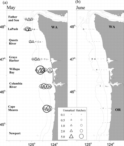
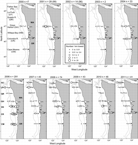
Overall, the average CPUE for juvenile steelhead during May surveys (1999–2011) was 0.5 fish/km towed (SD = 1). The CPUE was significantly higher in 2006 (3.7 fish/km towed) than in all other years (Kruskal–Wallis test: P < 0.0001); the CPUEs for the other years were not significantly different (Figure 2). Juvenile steelhead were captured along all transects across most years and were caught at the westernmost stations 49% of the time (Figure 2). The cross-shelf distribution of steelhead was highly variable among locations and among sampling years. Fish tended to be closer to shore (<32 km) at the southernmost transects and were more dispersed offshore at the northern transects. Juvenile steelhead CPUE increased with increasing salinity levels in surface waters (>28‰; Mann–Whitney U-test: P < 0.03; Figure 3).

FIGURE 3. Log(x + 0.1)-transformed CPUE (fish/km towed) for juvenile steelhead presented in relation to the surface salinity (‰; at 1 m) measured at the sampling station. The station was considered to be (1) in surface plume waters when salinity at 1-m depth was less than 28‰ or (2) outside of plume waters when salinity was greater than 28‰.

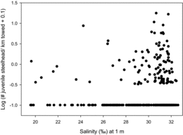
Table 2 Release and recovery information for coded-wire-tagged or PIT-tagged steelhead that were caught in marine waters off the coasts of Washington and Oregon. The mid-Columbia subbasin encompasses locations below the confluence of the Columbia and Snake rivers, including the Willamette and Umatilla rivers; the upper Columbia subbasin includes all tributaries above the confluence of the Columbia and Snake rivers. The Snake River basin includes all tributaries to the Snake River.

Release basin or subbasin	n	Days at large	Release latitude	Recovery location transects^a
Columbia River
Mid-Columbia subbasin	5	23.4	46°15′N	Cape Meares, Columbia River, Willapa Bay
Upper Columbia subbasin	5	28.8	46°15′N	Columbia River
Snake River	37	41.1	46°15′N	Cape Meares, Columbia River, Willapa Bay, La Push
Washington coast
Quinault River	7	33.5^b	47°55’N	Columbia River, Grays Harbor, Queets River
Sooes River	1	23	48°19’N	Columbia River

^aRecovery location transects are illustrated in Figure 1. The Columbia River transect includes data from special studies that sampled juvenile steelhead near the mouth of the Columbia River.^bFor two of the steelhead tagged in the Quinault River, the date of release was not provided in the coded wire tag database. Therefore, the number of days at large describes only the five fish with release date information.

Among the juvenile steelhead that were caught in marine waters, it was possible to determine origin and timing of release for 54 fish with CWTs and 3 fish with PIT tags (Table 2). Of these fish, all were of hatchery origin: 47 individuals originated from the Columbia River and 8 individuals originated from the Washington coast. Time between freshwater release and ocean recovery varied from 23.4 d for steelhead released from middle Columbia River hatcheries (Willamette and Umatilla rivers; n = 6) to 41.1 d (n = 36) for Snake River fish, although one fish was recovered in the year after release. Most of the sampled steelhead with CWTs were captured in marine waters west of their natal rivers (Table 2). Although over 75% of the fish were caught west of the Columbia River or northern Washington coast, there were exceptions. During the year with the highest ocean catches of juvenile steelhead (2006), eight Columbia River steelhead (from the Snake River and middle Columbia River) were found south of the Columbia River in Oregon coastal waters. Furthermore, catches of juvenile steelhead from the Columbia River estuary may not be directly comparable with catches from the ocean because some of the ocean-captured juveniles were not of Columbia River origin; 87.0% of the ocean-caught steelhead with CWTs originated from the Columbia River, but we also captured coded-wire-tagged fish from coastal Washington hatcheries. None of the coastal Oregon hatcheries applied CWTs to their steelhead.

Otolith structural and elemental data were available for 47 fish sampled in 2006; we calculated marine residence times for these fish. Only about half of the steelhead (n = 23) displayed elevated Sr:Ca at the otolith margin. The remaining 24 fish either displayed elevated Sr:Ca along the entire growth axis (n = 1) or no elevation of Sr:Ca (n = 23). Previous laboratory experiments (Zimmerman 2005; Miller 2011) indicated a rapid change in Sr:Ca of juvenile salmonids within 1–3 d after exposure to saline waters. Therefore, we assumed that individuals with no elevation of Sr:Ca at the otolith edge had been in marine waters for less than 3 d. Juvenile steelhead spent an average of 9.8 d (SD = 10.2) in the ocean prior to capture (Table 3). We calculated freshwater and marine migration rates for the four individuals with both CWTs and otolith information; the mean freshwater migration rate ranged from 10.0 to 38.0 km/d, and the marine migration rate (assuming linear distance between the point of marine entry and the capture location) ranged from 1.5 to 43.0 km/d.

Table 3 Size, growth, and residence parameters calculated based on otolith structural and elemental data from 47 juvenile steelhead collected off the coasts of Washington and Oregon. Hatchery fish had adipose fin clips and/or coded wire tags.

Variable	n	Mean	SD	Min	Max
Hatchery steelhead
Size at freshwater emigration (FL, mm)	16	224.3	24.6	174	250.7
Marine growth (% per day, mm)	16	0.15	0.03	0.12	0.2
Marine growth (mm/d)	16	0.33	0.06	0.24	0.49
Size at capture (FL, mm)	36	229.4	21.54	178	259.8
Day of capture	36	145.6	1.9	144	150
Marine residence period (d)	36	9.9	10.5	3	33
Day of freshwater emigration	36	135.63	10.1	112	147
Unmarked steelhead
Size at freshwater emigration (FL, mm)	5	211.4	46.3	134	252.1
Marine growth (% per day, mm)	5	0.14	0.03	0.1	0.17
Marine growth (mm/d)	5	0.3	0.09	0.21	0.4
Size at capture (FL, mm)	11	212.7	34.3	137.2	264.9
Day of capture	11	146	2.1	144	150
Marine residence period (d)	11	9.4	9.8	3	32.2
Day of freshwater emigration	11	136.7	8	117.8	143

FIGURE 4. Composition of the diet consumed by juvenile steelhead off the coasts of Oregon and Washington, 2000–2011. Fish prey taxa are shown in color, whereas other taxa are shown in grayscale. The “other” category includes arachnids, cirripedes (barnacle larvae), mysids, polychaetes, isopods, and gelatinous material. The “other teleosts” category includes clupeids, gadids, salmonids, osmerids, and other unidentified fish (including fish tissue and parts). Unidentified crustacean parts and material, fish scales, unidentified material, plant material, and plastic were excluded from the analysis. See Appendix Table A.1 for common names of taxa.

Diet Composition and Feeding Intensity

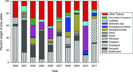
Most of the steelhead that were caught in the Columbia River estuary either had no food in their stomachs or had only small amounts of food. In the estuary, steelhead primarily ate common estuarine gammarid amphipods (Americorophium spp.) and insects. In the ocean, juvenile steelhead ate a wide variety of prey, including fish, euphausiids, and decapods, many of which have a neustonic distribution (Figure 4; Appendix Table A.1). The dominant prey group in terms of number eaten was a pelagic pteropod (sea butterfly Limacina helicina; 23.3%), followed by euphausiids (13.4%), fishes (13.6%), and crab Cancer spp. megalopae (10.2%). However, in terms of biomass contribution to the diet, L. helicina was relatively unimportant (<5.0%), whereas fishes (55.3%), euphausiids (20.3%), and Cancer spp. megalopae (9.8%) were the dominant prey categories (Figure 4; Appendix Table A.1). Among the identified fish taxa consumed, juvenile rockfishes (11–54 mm TL) occurred most frequently and were the most important fish prey in terms of weight consumed, followed by juvenile Sablefish (11–38 mm TL; Appendix Table A.1). Among the largest fish prey consumed were Pacific Sand Lances (up to 65 mm TL), Kelp Greenling Hexagrammos decagrammus (up to 60 mm TL), and two juvenile Chum Salmon (53 and 55 mm TL).

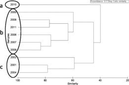
The SIMPROF analysis of annual ocean diet composition by weight indicated clustering of the diets into three significant year groupings (Figure 5): 2010 (cluster a); 2000, 2006–2009, and 2011 (cluster b); and 2001, 2002, and 2004 (cluster c). When incorporating fine-scale diet information at the sampling station level and testing for annual differences, the overall differences were significant (ANOSIM: global R = 0.86, P = 0.001) and were driven by the difference between clusters b and c. In general, the same prey groups were present in the diet during all years, but the prey taxa with the greatest contributions to the diet differed (Figure 5). In cluster a, the diets had large proportions of other fish and rockfishes. In cluster b, the diets included a large proportion of fish as well as many euphausiids. Cluster c was characterized by a higher proportion of decapods, mostly Dungeness crab Cancer magister megalopae, in the diets. There was no significant difference in diet between hatchery steelhead and unmarked steelhead during 2006, the only year in which there were enough fish from both groups to allow a comparison (ANOSIM: P > 0.05 for all station comparisons).

FIGURE 5. Cluster analysis using the similarity profile (SIMPROF) procedure, which identified three groupings of yearly average diets for juvenile steelhead collected off the coasts of Washington and Oregon.

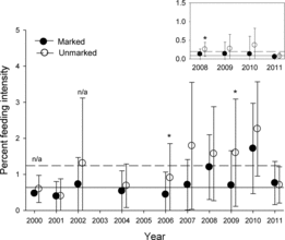
Indicators of future growth potential for juvenile steelhead can be measured based on the amount of food eaten (IFI) and the proportion of steelhead with empty stomachs. In the estuary, close to half of the fish had empty stomachs: only 40% of the hatchery steelhead and 53.3% of the unmarked fish had any food in their stomachs. In contrast, the majority of the ocean-caught steelhead (87.9% of hatchery fish; 92.3% of unmarked fish) had food in their stomachs. Additionally, in all years, steelhead that were caught in the ocean had eaten significantly more food than steelhead that were caught in the estuary (Kruskal–Wallis test: P < 0.05; Figure 6). The IFI of ocean-caught hatchery steelhead (0.7%; SD = 0.8%) was eight times higher than that of estuary-caught hatchery fish (0.09%; SD = 0.23%), and the IFI of ocean-caught unmarked fish (1.2%; SD = 1.3%) was six times higher than that of unmarked fish caught in the estuary (0.2%, SD = 0.3%; Figure 6). Lastly, unmarked steelhead had higher IFI values than hatchery fish in a given habitat. Among ocean-caught steelhead, unmarked fish had a higher IFI than hatchery fish—significantly so in 2006 and 2009 (Kruskal–Wallis test: P < 0.0001). Among individuals that were captured in the estuary, unmarked fish had a higher IFI than hatchery fish, and the difference was significant in 2008 (Kruskal–Wallis test: P = 0.001; Figure 6).

FIGURE 6. Annual means (±SE) of feeding intensity (weight of prey expressed as a percentage of total body weight) for hatchery (marked; filled circles) and unmarked (open circles) steelhead sampled in the ocean off the coasts of Oregon and Washington (main panel) and in the Columbia River estuary (inset) from 2000 to 2011. Horizontal lines are the overall means across all years for marked steelhead and unmarked fish. An asterisk indicates a significant difference between marked and unmarked fish in that year and habitat. Ocean data are not shown for 2003 or 2005 because too few fish were captured during those years.

Size, Condition, and Growth

Overall, there was little change in FL between steelhead caught in the estuary and those caught in the ocean during any given year (Figure 7a). Steelhead that were sampled from the estuary averaged 212.9 mm FL (SD = 27.8), whereas those captured in the ocean averaged 217.5 mm FL (SD = 26.7). There were several years in which ocean-caught steelhead were significantly longer than estuary-caught fish (Mann–Whitney test: 2011, all fish, P < 0.001; 2010, unmarked fish, P = 0.02; Figure 7a), but the FL differences were small. In samples from the ocean, fish of hatchery origin were significantly longer than unmarked fish except during 2010 and 2011 (Mann–Whitney test: P < 0.05; Figure 7a). On average, ocean-caught hatchery fish were 22.3 mm longer than ocean-caught unmarked fish; estuary-caught hatchery fish were 23.4 mm longer than estuary-caught unmarked fish.

FIGURE 7. Annual means (±SE) of (a) FL, (b) body condition residual (condition index), and (c) insulin-like growth factor 1 (IGF-1) for hatchery (marked; filled circles) and unmarked (open circles) steelhead caught in the ocean (main panels) or in the Columbia River estuary (insets). Horizontal lines are the overall means across years for hatchery steelhead and unmarked fish. An asterisk indicates a significant difference between hatchery and unmarked fish in that year and habitat; “n/a” means that too few data were available to test for significance.

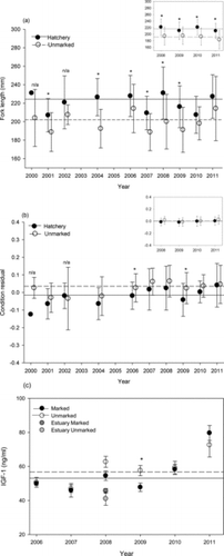
Although differences in length between ocean- and estuary-captured steelhead were generally small, the condition index of ocean-caught fish was significantly higher than that of estuary-caught fish. Ocean fish (both hatchery and unmarked) weighed more for a given body length than estuary fish (all years except 2009 hatchery fish; Mann–Whitney test: P < 0.05; Figure 7b). Estuary-caught steelhead had relatively uniform physical condition with little interannual variability (ANOVA: P > 0.05; Figure 7b), whereas ocean-caught steelhead showed significant differences in the condition index among years. Ocean-captured steelhead were in significantly better condition than estuary-caught individuals during 2007 and 2008 (hatchery and unmarked fish) and 2011 (hatchery fish only; ANOVA: P < 0.05). Among steelhead that were captured in the ocean, unmarked fish had a higher average body condition than hatchery fish across all years, and the difference was significant in 2006 and 2009 (Mann–Whitney test: P < 0.05; Figure 7b). This was not the case for steelhead in the estuary, as the condition index of unmarked fish was not significantly different from that of hatchery fish (Mann–Whitney test: P > 0.05; Figure 7b). Lastly, annual values of steelhead condition were compared with diet composition (ocean only) to determine whether changes in physical condition were related to diet. Average annual body condition of juvenile steelhead was significantly related to annual diet composition based on multidimensional scaling axis 1 scores (r² = 0.69; P = 0.004). During years when the ocean diets were primarily in cluster b (see Figures 4, 5), the condition of juvenile steelhead in the ocean was higher.

Growth data based on IGF-1 hormone levels were collected for ocean-caught steelhead in 2006–2011 and for estuary-caught steelhead in 2008. Both unmarked and hatchery steelhead in the ocean had significantly higher IGF-1 levels than estuary-caught fish during 2008 (Kruskal–Wallis test: P < 0.05; Figure 7c). Unmarked fish typically had higher IGF-1 levels than hatchery fish during all years and in both estuarine and ocean habitats, but the difference was significant only for 2009 (Kruskal–Wallis test: P = 0.03). Interannual differences in IGF-1 levels followed a similar pattern between hatchery fish and unmarked fish that were captured in the ocean: hormone levels in 2011 were significantly higher than those in other years, and levels in 2007 were the lowest (Kruskal–Wallis test: P < 0.05; Figure 7c). The IGF-1 levels in juvenile steelhead were positively related to body condition (r² = 0.47; P < 0.0001) and stomach fullness (r² = 0.19; P = 0.0002).

Analysis of otolith elemental data identified a group of juvenile steelhead that had resided in marine waters for more than 3 d, and otolith structures from these fish were used to calculate marine growth rates. The average size at freshwater emigration was 224.3 mm FL (SD = 24.6) for hatchery juveniles and 211.4 mm (SD = 46.3) for unmarked juveniles (Table 3). Estimated marine growth rates for hatchery fish (0.33 mm/d) and unmarked fish (0.30 mm/d; Table 3) were similar, although sample sizes for unmarked fish were low.

Table 4 Biological characteristics of ocean-caught juvenile steelhead in relation to capture distance from shore averaged in 8-km blocks. For each biological characteristic (FL, condition index, etc.), we tested for differences between 8-km blocks; for a given variable, values without a letter in common were significantly different (ANOVA: P < 0.05). No significant among-block differences in FL or insulin-like growth factor 1 (IGF-1) were found for unmarked fish.

	Distance from shore (8-km blocks)
Variable	8 km	16 km	24 km	32 km	40 km	48 km
Hatchery steelhead
FL (mm)	212.47 zyx	216.17 z	218.71 zy	222.28 x	224.92 z	232.17 yx
Condition residual	−0.0337 zy	−0.0358 z	−0.0077 yx	−0.02 zy	−0.0074 yx	0.0243 x
IGF-1 (ng/mL)	41.3 z	46.7 zy	52.1 yx	54.5 x	54.2 x	68.4 w
Stomach fullness (%)	0.29 z	0.48 zy	0.62 yx	0.74 x	1.0 w	1.03 w
Unmarked steelhead
FL (mm)	186.8462	201.7222	208.3333	213.7451	215.0244	217
Condition residual	−0.027 z	−0.002 z	0.049 y	0.066 y	0.013 z	0.062 y
IGF-1 (ng/mL)	43.7816	53.238	55.342	60.2274	55.8742	61.3537
Stomach fullness (%)	0.28 z	0.75 zy	1.5 zyx	1.3 x	1.6 yx	1.16 x

FIGURE 8. Means (±SE) for the relationship between capture site distance from shore (km) and the (a) mean FL, (b) body condition residual (condition index), (c) insulin-like growth factor 1 (IGF-1), and (d) percent feeding intensity for hatchery (filled circles) and unmarked (open circles) steelhead juveniles. Distances offshore were rounded to the nearest 8-km station for ease of visualizing the patterns. Sample sizes of hatchery and unmarked fish are shown above or below the symbols.

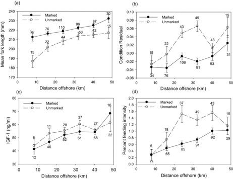
The capture distance offshore for ocean-caught juvenile steelhead (hatchery and unmarked fish) was compared with the biological characteristics of IFI, size, condition index, and growth (Figure 8). As juvenile hatchery steelhead migrated further offshore, the IFI, condition index, and IGF-1 all increased significantly (ANOVA: P < 0.05; Table 4). Unmarked juveniles had significantly fuller stomachs and higher condition in offshore waters (ANOVA: P < 0.05; Table 4). In both hatchery and unmarked steelhead, there was an increase in FL for fish that were caught further offshore; however, the difference was not significant for unmarked fish. For hatchery fish, the condition index did not follow a pattern of increase with distance from shore (ANOVA: P < 0.05; Table 4; Figure 8).

DISCUSSION

We determined that juvenile steelhead moved quickly west from near-coastal habitats and were associated with shelf waters for only a short period after their migration from freshwater. Previous studies have indicated that juvenile steelhead migrate to sea in spring and utilize coastal marine waters in the northern California Current for a relatively short period as they migrate to offshore waters (see reviews by Brodeur et al. 2003 and Quinn 2005). Hartt and Dell (1986) reported that juvenile steelhead have marine distributions unlike those of other juvenile Pacific salmon. Juvenile steelhead migrate directly offshore during their first summer in marine waters, whereas other Pacific salmon are largely associated with the coastal margin when they first enter the ocean and migrate northward along the coast (Pearcy and Fisher 1990). High-seas tagging recoveries have identified that steelhead make more extensive offshore migrations in their first marine summer than any other Pacific salmonid (Quinn and Myers 2004).

Pearcy and Fisher (1990) conducted extensive purse-seine sampling in waters off Oregon and Washington during spring and summer 1981–1985. Their mean catch was less than 1.0 steelhead/set for all year × month combinations, but most of the steelhead were caught in May or early June. The CPUE was highest off the Columbia River, although fish were caught throughout the entire latitudinal range of sampling (48.4°N to 42.8°N; Cape Flattery in northern Washington to Cape Blanco in southern Oregon). Catches were generally highest at stations located more than 28 km from shore (Pearcy and Fisher 1990). Our results were consistent with patterns observed in these studies.

Juvenile steelhead appeared to spend about 10 d in our sampling area, whereas juveniles from some spring Chinook Salmon O. tshawytscha populations resided there closer to 30 d (Tomaro et al. 2012). Marine migration rates estimated in our study suggest that the migrating steelhead could reach the westward edge of the ocean sampling stations in just a few days. The May ocean surveys typically occurred during the last week of the month, but the peak out-migration of juvenile steelhead from the Columbia River occurs during mid-May (Weitkamp et al. 2012). Thus, the May ocean surveys for Columbia River steelhead juveniles may have undersampled the total population, as many of the fish could have moved beyond our ocean sampling grid by late May.

Additional evidence that we undersampled juvenile steelhead migrants in the marine environment comes from two studies. First, in the Columbia River estuary during spring, steelhead, Coho Salmon O. kisutch, and Chinook Salmon typically have similar abundances in the catch (Dawley et al. 1986; Weitkamp et al. 2012). However, steelhead abundance in the ocean catch during May is just a fraction of the Coho Salmon and Chinook Salmon abundances (oceanic abundance of salmon in the 1980s: Pearcy and Fisher 1990; oceanic abundance of Chinook Salmon: Daly et al. 2011; May abundance of Coho Salmon: E. A. Daly, unpublished data). Thus, steelhead abundance in our ocean catches appears to be disproportionally low compared with that in estuarine catches.

During the transition between freshwater and salt water (smoltification), steelhead exhibit clear changes in both behavior (including feeding) and physiology (Folmar and Dickhoff 1980). During the early ocean phase, Columbia River juvenile steelhead eat more, grow faster, and are in better condition than individuals in the estuary. Assuming that the steelhead caught at our two estuarine locations were representative of fish in the estuary as a whole, hatchery steelhead consumed relatively few prey and had a high percentage of empty stomachs, indicating that they were not feeding in the estuary to the same degree as in marine habitats. Likewise, estuary-caught unmarked fish had low to modest rates of food consumption relative to unmarked fish captured in the ocean. The low feeding rates observed for steelhead in the estuary were similar to those reported in an earlier study (Dawley et al. 1986).

In contrast to estuary-sampled juveniles, steelhead consumed increasing amounts of food and made substantial gains in growth and condition upon entering the ocean and moving offshore. A similar growth spurt was observed by MacFarlane (2010) between juvenile Chinook Salmon caught in the San Francisco Bay estuary and those caught further offshore. Although we did not measure the relative quality of prey in the two habitats, consumption of lipid-rich prey in the ocean may lead to higher growth and condition (Daly et al. 2010; MacFarlane 2010). Thus, the ability to move quickly through the estuary and into ocean habitats may confer survival benefits upon these juveniles.

Our analyses of the ocean diets of steelhead were consistent with the results of previous studies, which indicated that juvenile steelhead in the ocean have a broad diet consisting of invertebrate and fish prey. Pearcy et al. (1990) found that steelhead caught in purse seines off the coasts of Oregon and Washington consumed primarily fishes (mainly rockfishes, smelts, and sand lances by weight) and euphausiids. Euphausiids were especially prevalent during strong upwelling years and were the dominant prey consumed by a number of pelagic fish predators during those years (Brodeur and Pearcy 1992). Similarly, Miller and Brodeur (2007) found that steelhead juveniles collected off southern Oregon and northern California had substantially different diets during the 2 years sampled, with euphausiids dominating the diet in 2000 (84% of total prey weight) and fish dominating the diet in 2002 (57% of total prey weight).

As suggested by Pearcy et al. (1990), the types of prey eaten by juvenile steelhead occur mainly in the upper part of the water column—in many cases, the near-surface (<1 m) neustonic layer. Surface-oriented prey items include many pteropods, crab larvae, and primarily neustonic fishes (e.g., greenlings and Sablefish) as well as dead floating insects (Shenker 1988; Brodeur 1989; Pool and Brodeur 2006). The location of these prey types suggests that steelhead juveniles spend much of their time feeding very close to the surface, which may have implications for our sampling methodology. Tagging studies have shown that adult steelhead are surface oriented (Ruggerone et al. 1990). We may have undersampled steelhead that were situated higher in the water column than our net was able to fish (0.5–1.0 m below the surface; Krutzikowsky and Emmett 2005). Increased flotation on the headrope should be evaluated to improve the catchability of juvenile steelhead.

Interannual variability in the steelhead's diet has been linked to changes in growth in the North Pacific Ocean and the Gulf of Alaska (Atcheson et al. 2012). Using a bioenergetics model with field-based inputs, Atcheson et al. (2012) concluded that growth of steelhead in the ocean might be limited by prey availability and temperature. Our study results support the idea that changes in the ocean growth of steelhead as measured by body condition correspond with changes in diet composition. However, this relationship was tested during only a small window of marine residence (early juvenile stage). In contrast, Atcheson et al. (2012) illustrated that ocean conditions are also important during various stages of subadult and adult steelhead development.

Burla et al. (2010a) showed that interannual variability in the structure of the Columbia River plume was correlated with the survival of Columbia River steelhead juveniles (but not Chinook Salmon), although the authors did not suggest a mechanism that might explain why the two were related. Survival of juvenile steelhead increased when plume surface volume was larger and extended further offshore (versus more attached to shore; Burla et al. 2010a). Catches of steelhead in our study were higher outside the Columbia River plume than inside the plume, suggesting quick migration through plume waters. Our biological metrics of feeding and growth showed improvement as juvenile steelhead migrated westward from the point of ocean entry.

Juvenile steelhead may actively or passively utilize plume waters to speed their transit out of estuaries and nearshore waters and into marine habitat with enhanced foraging and growth potential. Upon ocean entry, juvenile steelhead swam quickly westward into shelf waters, where production of prey fish larvae and juveniles is higher than that in coastal waters (Auth 2008). Utilization of coastal plume dynamics to quickly migrate offshore into richer feeding grounds could greatly improve the survival of juvenile steelhead in our coastal region. Experimental variations in river discharge during out-migration of ESA-listed steelhead should be evaluated as a potential adaptive management practice.

Low river discharge and plume volume would likely increase steelhead residence time in the estuary and nearshore coastal waters, where feeding and growth were reduced, thus increasing the vulnerability of these fish to size-selective predation. The higher capture rate of marked steelhead in the estuary than in the ocean suggests that some fraction of the hatchery population was not accounted for in our ocean sampling. A higher proportion of wild Chinook Salmon was sampled in the shallow beach areas of the estuary relative to collections from the estuary channel, suggesting that the wild fish were closer to shore (Roegner et al. 2012; Weitkamp et al. 2012). In addition, we know that part of our ocean catch included fish from Washington coastal rivers, where marking rates are lower (Oregon rates are higher). However, evidence from the recovery of PIT tags on seabird colonies suggests that steelhead smolts are particularly vulnerable to avian predators in the estuary, possibly due to their greater tendency toward surface orientation compared with other salmonids (Collis et al. 2001; Ryan et al. 2003; Evans et al. 2012). The ratio of unmarked to marked steelhead in our catches was higher in the ocean than in the estuary, which suggests that naturally produced steelhead are potentially surviving at a higher rate than hatchery fish. Some studies have reported higher survival rates for wild salmon than for hatchery fish (Chittenden et al. 2008; Beamish et al. 2012; Claiborne 2013), whereas other studies have not detected survival differences (Thorstad et al. 2007; Johnson et al. 2010). Directed studies on the survival rates of wild and hatchery-origin juvenile steelhead in our study region are warranted.

Steelhead susceptibility to predation by a dominant avian predator in the estuary, the Caspian tern Hydroprogne caspia, was shown to be a function of size (peaking at 202 mm) but was also inversely related to steelhead condition and to the river discharge rate (Hostetter et al. 2012). Predation rates in coastal waters are virtually unknown (K. W. Myers, University of Washington, personal communication), but increases in feeding, condition, and growth of steelhead in offshore waters may also be due to predators’ removal of the less-fit juvenile steelhead from inshore waters; this possibility remains to be examined.

Our ability to differentiate hatchery fish from naturally produced fish is confounded by current hatchery management practices, whereby a certain percentage of fish are released without external marks. During this study, we attempted to identify differences between hatchery steelhead and unmarked steelhead, the latter of which may have included some hatchery fish in addition to the naturally produced individuals. Despite the incomplete marking of hatchery fish, we were still able to detect differences between hatchery steelhead and unmarked fish in most of the physical metrics examined. In both the estuary and ocean, hatchery steelhead were longer on average than unmarked fish, although the condition of unmarked fish was generally higher than that of hatchery fish. Unmarked steelhead also had slightly higher IGF-1 and IFI values than hatchery fish, whereas diet composition did not differ between the two groups. In a similar study, Daly et al. (2011) observed this same pattern for hatchery and unmarked juveniles of Columbia River spring Chinook Salmon during early marine residence. Recent research has identified that the adipose fin—traditionally thought to be vestigial and nonfunctional—may serve a useful purpose for swimming performance (Buckland-Nicks et al. 2012). As such, the feeding and growth differences between marked steelhead and unmarked steelhead (naturally produced fish and unclipped hatchery fish) may in part be due to the intact adipose fins of the latter group.

For both juvenile steelhead (present study) and juvenile Columbia River spring Chinook Salmon (Daly et al. 2012), unmarked individuals had smaller FLs but better body condition, fuller stomachs, and higher IGF-1 levels than their hatchery counterparts. Although diet composition did not appear to differ between hatchery and unmarked fish in both studies, those results were in contrast to the findings of Quinn et al. (2012), who examined stable isotope ratios and determined that wild steelhead fed at a higher trophic level and depended on more nearshore-derived prey sources than did hatchery fish. It should be noted, however, that the samples in the Quinn et al. (2012) study were taken from adult steelhead that had returned to freshwater to spawn, and any such feeding differences could have happened later in the marine life history rather than at initial ocean entry. If unmarked fish are eating more and growing at a higher rate than hatchery fish in the marine environment, this could provide a survival advantage to the naturally produced fish.

Our biological comparisons of Columbia River estuary-caught steelhead with ocean-caught steelhead may have been influenced by the fact that steelhead originating from coastal Washington and perhaps Oregon rivers were present in ocean samples. Baseline information on genetic stock identification of steelhead from coastal Washington and Oregon is needed to augment the data currently available from Columbia River steelhead populations (e.g., Blankenship et al. 2011). This information would enhance the ability of resource managers to identify differences among these populations. Additional otolith chemistry and structural data are also needed to increase our understanding of juvenile steelhead marine growth and coastal ocean migration rates at this critical time.

An understanding of which estuary, plume, and ocean conditions are important for steelhead migration, feeding, and growth is critical for the management and restoration of declining populations. Recovery planning will require a better understanding of sequential habitats that are important for optimal growth and survival during the migration from freshwater to oceanic environments. Steelhead migrate through estuary and coastal ocean waters during a narrow window of time; this behavior is different from that of other salmonid species, which tend to exhibit extended migration periods and residence times in coastal waters. Effective management practices for the improvement of endangered or threatened steelhead populations would require explicit information about where these fish go and how they adapt once they reach the ocean. Our data begin to address these unknowns.

ACKNOWLEDGMENTS

We thank the captains and crews of the research and chartered fishing vessels for their assistance at sea, along with the many scientists who collected and processed the steelhead at sea and in the laboratory. We are indebted to Gabi Kraller, Sylvia Pauly, and Megan Sabal for assistance with laboratory analysis of stomach contents; Larissa Rohrbach for IGF-1 sample collection and processing; and Stefanie Gera (National Science Foundation, Research Experiences for Undergraduates) for assistance with otolith processing. We also thank the Bonneville Power Administration and NOAA Northwest Fisheries Science Center for long-term funding of this project. The manuscript was greatly improved by comments provided by S. Hayes, K. Fresh, T. Quinn, and an anonymous reviewer.

APPENDIX: Frequency of Occurrence and Taxonomic Composition of prey in Steelhead Diets

Percent frequency of occurrence (FO), percent composition by number (N), and percent composition by weight (W) of prey taxa in stomachs of juvenile steelhead captured off the coasts of Oregon and Washington for all years combined (including steelhead from the Columbia River plume front study in 2001–2002). Unidentified material is not included in the table. Asterisks indicate prey taxa that were also present in the stomachs of steelhead collected in the Columbia River estuary. Unidentified caddisflies (Trichoptera) were also present in the diets of estuary-caught steelhead but were not found in the diets of ocean-caught fish.

Table

Prey taxon	FO (%)	N (%)	W (%)
Annelida
Unidentified Polychaeta*	0.50	0.08	0.27
Mollusca
Gastropoda:
Sea butterfly Limacina helicina*	1.45	23.28	4.69
Unidentified Pteropoda*	0.20	0.30	0.26
Arthropoda
Copepoda:
Neocalanus cristatus	0.05	0.32	0.02
Unidentified Calanoida	0.35	1.76	0.44
Unidentified Copepoda	0.65	0.41	0.09
Cirripedia:
Unidentified Cirripedia	0.15	3.48	0.04
Gooseneck barnacles Lepas spp.	0.15	3.48	0.04
Mysidacea:
Unidentified Mysidacea	0.10	0.02	0.01
Isopoda:
Idotea spp.	0.05	0.01	0.00
Idotea fewkesi	0.05	0.02	0.06
Unidentified Isopoda*	0.15	0.02	0.01
Amphipoda:
Atylus tridens	1.50	0.44	0.19
Americorophium spp.*	0.10	0.02	0.00
Unidentified Gammaridae*	1.80	0.76	0.15
Brachyscelus crusculum	0.05	0.02	0.03
Hyperia medusarum	0.35	0.12	0.08
Hyperoche medusarum	3.95	1.84	0.37
Lycaea pulex	0.15	0.02	0.00
Primno macropa	0.15	0.04	0.02
Themisto pacifica	0.15	0.03	0.00
Vibilia spp.	0.05	0.01	0.00
Vibilia australis	0.05	0.49	0.03
Vibilia pyripes	0.15	0.31	0.05
Unidentified Hyperiidea	4.85	1.78	0.61
Unidentified Amphipoda	0.05	0.04	0.01
Euphausiacea (krill):
Euphausia pacifica	5.55	4.53	7.27
Thysanoessa spinifera	4.40	1.65	4.07
Unidentified Euphausiacea*	10.65	7.26	8.99
Decapoda:
Unidentified Brachyura zoeae	0.20	0.08	0.00
Crab Cancer spp. megalopae	2.70	1.06	0.92
Dungeness crab Cancer magister megalopae	10.25	8.04	8.47
Pygmy rock crab Cancer oregonensis/red rock crab Cancer productus megalopae	3.15	1.07	0.40
Unidentified Pandalidae	0.15	0.02	0.00
Unidentified Decapoda	1.30	0.45	0.41
Insecta:
Aphidae	0.05	0.01	0.01
Coleoptera*	0.65	0.14	0.09
Diptera*	0.15	0.03	0.00
Hymenoptera	0.15	0.06	0.04
Homoptera	0.05	0.01	0.02
Unidentified Insecta*	5.45	1.28	0.83
Arachnida:
Unidentified Araneae (spiders)	0.05	0.01	0.00
Unidentified Arachnida*	0.05	0.01	0.00
Chordata
Osteichthyes:
Unidentified Clupeidae	0.10	0.02	0.05
Chum Salmon Oncorhynchus keta	0.05	0.02	0.80
Unidentified Osmeridae	0.05	0.02	0.06
Pacific Tomcod Microgadus proximus	0.05	0.01	0.06
Pacific Saury Cololabis saira	0.05	0.01	0.06
Pacific Sand Lance Ammodytes hexapterus	1.55	0.65	3.35
Rockfishes Sebastes spp.	3.45	1.33	12.02
Sablefish Anoplopoma fimbria	2.35	2.38	5.94
Kelp Greenling Hexagrammos decagrammus	0.85	0.24	3.36
Lingcod Ophiodon elongatus	0.20	0.06	0.48
Unidentified Hexagrammidae	1.00	0.30	3.45
Irish lords Hemilepidotus spp.	0.80	0.27	0.97
Brown Irish Lord Hemilepidotus spinosus	0.50	0.14	0.61
Cabezon Scorpaenichthys marmoratus	0.65	0.15	0.61
Unidentified Cottidae	1.35	0.53	1.16
Unidentified Pleuronectidae	0.10	0.02	0.07
Unidentified Osteichthyes*	14.86	6.50	22.28
Gelatinous material	0.10	0.05	0.02
Number of stomachs examined		671
Number of empty stomachs		30
Mean FL (mm)		216.7
FL range (mm)		138–290

REFERENCES

- Atcheson, M., K.W. Myers, D.A. Beauchamp, and N.J. Mantua. 2012. Bioenergetic response by steelhead to variation in diet, thermal habitat, and climate in the North Pacific Ocean. Transactions of the American Fisheries Society 141:1081–1096.
- Augerot, X. 2005. Atlas of Pacific salmon. University of California Press, Berkeley.
- Auth, T.D.> 2008. Distribution and community structure of ichthyoplankton from the northern and central California Current in May 2004–06. Fisheries Oceanography 17:316–331.
- Beamish, R.J.>, R.M. Sweeting, C.M. Neville, K.L. Lange, T.D. Beacham, and D. Preikshot. 2012. Wild Chinook Salmon survive better than hatchery salmon in a period of poor production. Environmental Biology of Fishes 94:135–148.
- Beckman, B.R.>, W. Fairgrieve, K.A. Cooper, C.V. W. Mahnken, and R.J. Beamish. 2004a. Evaluation of endocrine indices of growth in individual postsmolt Coho Salmon. Transactions of the American Fisheries Society 133:1057–1067.
- Beckman, B.R.>, M. Shimizu, B.A. Gadberry, P.J. Parkins, and K.A. Cooper. 2004b. The effect of temperature change on the relations among plasma IGF-1, 41-kDa IGFBP, and growth rate in postsmolt Coho Salmon. Aquaculture 241:601–619.
- Blankenship, S.M.>, M.R. Campbell, J.E. Hess, M.A. Hess, T.K. Kassler, C.C. Kozfkay, A.P. Matala, S.R. Narum, M.M. Paquin, M.P. Small, J.J. Stephenson, and K.I. Warheit. 2011. Major lineages and metapopulations in Columbia River Oncorhynchus mykiss are structured by dynamic landscape features and environments. Transactions of the American Fisheries Society 140:665–684.
- Bond, M.H.>, S.A. Hayes, C.V. Hanson, and R.B. MacFarlane. 2008. Marine survival of steelhead (Oncorhynchus mykiss) enhanced by a seasonally closed estuary. Canadian Journal of Fisheries and Aquatic Sciences 65:2242–2252.
- Brodeur, R.D.> 1989. Neustonic feeding by juvenile salmonids in coastal waters of the northeast Pacific. Canadian Journal of Zoology 67:1995–2007.
- Brodeur, R.D.>, J.P. Fisher, C.A. Morgan, R.L. Emmett, and E. Casillas. 2005. Species composition and community structure of pelagic nekton off Oregon and Washington under variable oceanographic conditions. Marine Ecology Progress Series 298:41–57.
- Brodeur, R.D.>, K.W. Myers, and J.H. Helle. 2003. Research conducted by the United States on the early life history of Pacific salmon. Bulletin of the North Pacific Anadromous Fish Commission 3:89–131.
- Brodeur, R.D.>, and W.G. Pearcy. 1992. Effects of environmental variability on trophic interactions and food web structure in a pelagic upwelling ecosystem. Marine Ecology Progress Series 84:101–119.
- Buckland-Nicks, J.A.>, M. Gills, and T.E. Reimchen. 2012. Neural network detected in a presumed vestigial trait: ultrastructure of the salmonid adipose fin. Proceedings of the Royal Society B 279:553–563.
- Burgner, R.L.>, J.T. Light, L. Margolis, T. Okazaki, and S. Ito. 1992. Distribution and origins of steelhead trout (Oncorhynchus mykiss) in offshore waters of the North Pacific Ocean. International North Pacific Fisheries Commission Bulletin 51.
- Burla, M., A.M. Baptista, E. Casillas, J.G. Williams, and D.M. Marsh. 2010a. The influence of the Columbia River plume on the survival of steelhead (Oncorhynchus mykiss) and Chinook Salmon (Oncorhynchus tshawytscha): a numerical exploration. Canadian Journal of Fisheries and Aquatic Sciences 67:1671–1684.
- Burla, M., A.M. Baptista, Y.L. Zhang, and S. Frolov. 2010b. Seasonal and interannual variability of the Columbia River plume: a perspective enabled by multiyear simulation databases. Journal of Geophysical Research: Oceans [online serial] 115:C00B16.
- Busby, P.J.>, T.C. Wainwright, G.J. Bryant, L.J. Lierheimer, R.S. Waples, F.W. Waknitz, and I.V. Lagomarsino. 1996. Status review of west coast steelhead from Washington, Idaho, Oregon, and California. NOAA Technical Memorandum NMFS-NWFSC-27.
- Campana, S.E.> 1982. Feeding periodicity and the production of daily growth increments in otoliths of steelhead trout (Salmo gairdneri) and Starry Flounder (Platichthys stellatus). Canadian Journal of Zoology 61:1591–1597.
- Chittenden, C.M. S.>, S. Sura, K.F. Butterworth, K.F. Cubitt, N. Plantalech Manel-la, F.O. Balfry, and R.S. McKinley. 2008. Riverine, estuarine, and marine migratory behavior and physiology of wild and hatchery reared Coho Salmon Oncorhynchus kisutch (Walbaum) smolts descending the Campbell River, BC, Canada. Journal of Fish Biology 72:614–628.
- Claiborne, A.M.> 2013. A comparison of early marine residence in hatchery and natural Chinook Salmon (Oncorhynchus tshawytscha).. Master's thesis. Oregon State University, Corvallis.
- Clarke, K.R.> 1993. Non-parametric multivariate analysis of changes in community structure. Australian Journal of Ecology 18:117–143.
- Clarke, K.R.>, and R.M. Warwick. 2001. Change in marine communities: an approach to statistical analysis and interpretation, 2nd edition. Primer-E, Plymouth Marine Laboratory, Plymouth, UK.
- Collis, K., D.D. Roby, D.P. Craig, B.A. Ryan, and R.D. Ledgerwood. 2001. Colonial waterbird predation on juvenile salmonids tagged with passive integrated transponders in the Columbia River estuary: vulnerability of different salmonid species, stocks, and rearing types. Transactions of the American Fisheries Society 130:385–396.
- Daly, E.A.>, C.E. Benkwitt, R.D. Brodeur, M.N. C. Litz, and L. Copeman. 2010. Fatty acid profiles of juvenile salmon indicate prey selection strategies in coastal marine waters. Marine Biology 157:1975–1987.
- Daly, E.A.>, R.D. Brodeur, J.P. Fisher, L.A. Weitkamp, D.J. Teel, and B.R. Beckman. 2011. Spatial and trophic overlap of marked and unmarked Columbia River basin spring Chinook Salmon during early marine residence with implications for competition between hatchery and naturally produced fish. Environmental Biology of Fishes 94:117–134.
- Dawley, E.M.>, R.D. Ledgerwood, T.H. Blahm, C.W. Sims, J.T. Durkin, R.A. Kirn, G.E. Monan, and F.J. Ossiander. 1986. Migrational characteristics, biological observations, and relative survival of juvenile salmonids entering the Columbia River estuary, 1966–1983. Final Report to the Bonneville Power Administration, Project 81-102, Portland, Oregon and the National Oceanic and Atmospheric Administration, National Marine Fisheries Service, Coastal Zone and Estuarine Studies Division, Seattle.
- De Robertis, A., C.A. Morgan, R.A. Schabetsberger, R.W. Zabel, R.D. Brodeur, R.L. Emmett, C.M. Knight, G.K. Krutzikowsky, and E. Casillas. 2005. Columbia River plume fronts II. Distribution, abundance, and feeding ecology of juvenile salmon. Marine Ecology Progress Series 299:33–44.
- Evans, A.F.>, N.J. Hostetter, D.D. Roby, K. Collis, D.E. Lyons, B.P. Sandford, R.D. Ledgerwood, and S. Sebring. 2012. Systemwide evaluation of avian predation on juvenile salmonids from the Columbia River based on recoveries of passive integrated transponder tags. Transactions of the American Fisheries Society 141:975–989.
- Folmar, L.C.>, and W.W. Dickhoff. 1980. The parr-smolt transformation (smoltification) and seawater adaptation in salmonids: a review of selected literature. Aquaculture 21:1–37.
- Francis, R.I. C. C.> 1990. Back-calculation of fish length: a critical review. Journal of Fish Biology 36:883–902.
- Hartt, A.C.>, and M.B. Dell. 1986. Early oceanic migrations and growth of juvenile Pacific salmon and steelhead trout. International North Pacific Fisheries Commission Bulletin 46.
- Hostetter, N.J.>, A.F. Evans, D.D. Roby, and K. Collis. 2012. Susceptibility of juvenile steelhead to avian predation: the influence of individual fish characteristics and river conditions. Transactions of the American Fisheries Society 141:1586–1599.
- Johnson, S.L.>, J.H. Power, D.R. Wilson, and J. Ray. 2010. A comparison of the survival and migratory behavior of hatchery-reared and naturally-reared steelhead smolts in the Alsea River and estuary, Oregon, using acoustic telemetry. North American Journal of Fisheries Management 30:55–71.
- Krutzikowsky, G.K.>, and R.L. Emmett. 2005. Diel differences in surface trawl fish catches off Oregon and Washington. Fisheries Research 71:365–371.
- MacFarlane, R.B.> 2010. Energy dynamics and growth of Chinook Salmon (Oncorhynchus tshawytscha) from the Central Valley of California during the estuarine phase and first ocean year. Canadian Journal of Fisheries and Aquatic Sciences 67:1549–1565.
- Miller, J.A.> 2011. Effects of water temperature and barium concentration on otolith composition along a salinity gradient: implications for migratory history. Journal of Experimental Marine Biology and Ecology 405:42–52.
- Miller, T.W.>, and R.D. Brodeur. 2007. Diets of and trophic relationships among dominant marine nekton within the northern California Current ecosystem. U.S. National Marine Fisheries Service Fishery Bulletin 105:548–559.
- Miller, J.A.>, A. Gray, and J. Merz. 2010. Quantifying the contribution of juvenile migratory phenotypes in a population of Chinook Salmon (Oncorhynchus tshawytscha). Marine Ecology Progress Series 408:227–240.
- Miller, D.R.>, J.G. Williams, and C.W. Sims. 1983. Distribution, abundance and growth of juvenile salmonids off the coast of Oregon and Washington, summer 1980. Fisheries Research 2:1–17.
- Moore, M.E.>, B.A. Berejikian, and E.P. Tezak. 2010a. Early marine survival and behavior of steelhead smolts through Hood Canal and the Strait of Juan de Fuca. Transactions of the American Fisheries Society 139:49–60.
- Moore, M.E.>, F.A. Goetz, D.M. Van Doornik, E.P. Tezak, T.P. Quinn, J.J. Reyes-Tomassini, and B.A. Berejikian. 2010b. Early marine migration patterns of wild Coastal Cutthroat Trout (Oncorhynchus clarki clarki), steelhead trout (Oncorhynchus mykiss), and their hybrids. PLoS One [online serial] 5:E12881.
- Pearcy, W.G.> 1992. Ocean ecology of North Pacific salmonids. University of Washington Press, Seattle.
- Pearcy, W.G.>, R.D. Brodeur, and J.P. Fisher. 1990. Distribution and biology of juvenile Cutthroat Trout (Oncorhynchus clarki clarki) and steelhead (O. mykiss) in coastal waters off Oregon and Washington. U.S.National Marine Fisheries Service Fishery Bulletin 88:697–711.
- Pearcy, W.G.>, and J.P. Fisher. 1990. Distribution and abundance of juvenile salmonids off Oregon and Washington, 1981–1985. NOAA Technical Report NMFS 93.
- Pool, S.S.>, and R.D. Brodeur. 2006. Neustonic macrozooplankton abundance and distribution in the Northern California Current, 2000 and 2002. NOAA Technical Memorandum NWFSC-74.
- Quinn, T.P.> 2005. The behavior and ecology of Pacific salmon and trout. University of Washington Press, Seattle.
- Quinn, T.P.>, and K.W. Myers. 2004. Anadromy and the marine migrations of Pacific salmon and trout: Rounsefell revisited. Reviews in Fish Biology and Fisheries 14:421–442.
- Quinn, T.P.>, T.R. Seamons, and S.P. Johnson. 2012. Stable isotopes of carbon and nitrogen indicate differences in marine ecology between wild and hatchery produced steelhead. Transactions of the American Fisheries Society 141:526–532.
- Roegner, G.C.>, R. McNatt, D.J. Teel, and D.L. Bottom. 2012. Distribution, size, and origin of juvenile Chinook Salmon in shallow-water habitats of the lower Columbia River and estuary, 2002–2007. Marine and Coastal Fisheries: Dynamics, Management, and Ecosystem Science [online serial] 4:450–472.
- Ruggerone, G.T.>, T.P. Quinn, I.A. McGregor, and T.S. Wilkinson. 1990. Horizontal and vertical movement of adult steelhead trout, Oncorhynchus mykiss, in Dean and Fisher channels, British Columbia. Canadian Journal of Fisheries and Aquatic Sciences 47:1963–1969.
- Ryan, B.A.>, S.G. Smith, J.M. Butzerin, and J.W. Ferguson. 2003. Relative vulnerability to avian predation of juvenile salmonids tagged with passive integrated transponders in the Columbia River estuary 1998–2000. Transactions of the American Fisheries Society 132:275–288.
- Shenker, J.M.> 1988. Oceanographic associations of neustonic larval and juvenile fishes and Dungeness crab megalopae off Oregon. U.S. National Marine Fisheries Service Fishery Bulletin 86:299–317.
- Shimizu, M., P. Swanson, H. Fukada, A. Hara, and W.W. Dickhoff. 2000. Comparison of extraction methods and assay validation for salmon insulin-like growth factor-I using commercially available components. General and Comparative Endocrinology 119:26–36.
- Thorstad, E.B.>, F. Oakland, B. Finstad, R. Sivertsgard, N. Plantalech, P.A. Bjorn, and R.S. McKinley. 2007. Fjord migration and survival of wild and hatchery-reared Atlantic Salmon and wild Brown Trout post-smolts. Hydrobiologia 582:99–107.
- Tomaro, L.M.>, D.J. Teel, W.T. Peterson, and J.A. Miller. 2012. When is bigger better? Early marine residence of middle and upper Columbia River spring Chinook Salmon. Marine Ecology Progress Series 452:237–252.
- Weitkamp, L.A.>, P.J. Bentley, and M.N. C. Litz. 2012. Seasonal and interannual variation in juvenile salmonids and associated fish assemblage in open waters of the lower Columbia River estuary. U.S. National Marine Fisheries Service Fishery Bulletin 110:426–450.
- Woodson, L., B.K. Wells, R.C. Johnson, P. Weber, R.B. MacFarlane, and G. Whitman. 2013. Evaluating selective mortality of juvenile Chinook Salmon (Oncorhynchus tshawytscha) across years of varying ocean productivity. Marine Ecology Progress Series 487:163–175.
- Wright, P.J.>, N.B. Metcalfe, and J.E. Thorpe. 1990. Otolith and somatic growth rates in Atlantic Salmon parr, Salmo salar L.—evidence against coupling. Journal of Fish Biology 36:241–249.
- Zimmerman, C.E.> 2005. Relationship of otolith strontium-to-calcium ratios and salinity: experimental validation for juvenile salmonids. Canadian Journal of Fisheries and Aquatic Sciences 62:88–97.