A Surplus Production Model Considering Movements between Two Areas using Spatiotemporal Differences in CPUE: Application to Sea Ravens Hemitripterus villosus off Fukushima as a Practical Marine Protected Area after the Nuclear Accident

Abstract

Although the number of marine protected areas (MPAs) for stock management has increased, movements or differences in population structure of a target species between an MPA and surrounding fishing areas have rarely been considered in stock biomass estimations. We developed a surplus production model considering seasonal movements between two areas; the model was applied to Sea Ravens Hemitripterus villosus off Fukushima, where almost all fishing has been prohibited since the 2011 accident at the Fukushima Dai-ichi Nuclear Power Plant. We predicted future biomass by using CPUE data from coastal gill-net fishing and offshore bottom trawl fishing in 2000 to 2009. The model reflected the seasonal coastal–offshore movements of Sea Ravens well, and it predicted increasing Sea Raven biomass in both areas, which was validated by the CPUEs observed after 2010—including those for trial bottom trawl fishing that occurred within limited offshore areas after the accident. Our results indicate that the newly developed model incorporating seasonal movements of Sea Ravens is feasible and that the waters off Fukushima have effectively been serving as an MPA since the nuclear accident. We also demonstrated the model's applicability for estimating the optimal fishing effort and designing a new MPA for stock management that considers seasonal movements.

Received August 29, 2014; accepted May 4, 2015

Spatially based effort management, such as no-take areas or rotating closures, has been widely recognized as a feasible stock management method for conserving biodiversity, ecosystem services, habitats, and endangered species as well as for increasing biomass (Agardy 1994; Allison et al. 1998; Jones 2001; Halpern and Warner 2002; Field et al. 2006; Lester et al. 2009). Marine protected areas (MPAs) are one of the management methods currently used. They are defined as areas with legal boundaries in which fishing is prohibited for all or a subset of a species, or where particular fishing gears are disallowed with some degree of permanence (Field et al. 2006). In line with global targets agreed upon by the Convention on Biological Diversity, the number of MPAs is increasing rapidly (Edgar et al. 2014).

Virtual population analysis and surplus production models have been widely used to assess fish abundance (Hilborn and Walters 1992; Coggins et al. 2006). In general, these models assume that the assessed population has a high diffusivity, which means that the effects of local recruitment events and regional fisheries spread rapidly throughout the entire stock (Field et al. 2006). However, the establishment of an MPA is expected to generate heterogeneous patterns of abundance, age structure, and size structure inside and outside of the MPA, especially in less-migratory species with strong local retention mechanisms (Guénette et al. 1998; Holland 2002; Punt and Methot 2004; Hart 2006). Consequently, the development of stock assessment models that can incorporate spatial differences in population structure and movement patterns in waters within and outside of MPAs may be necessary in some special cases (Field et al. 2006).

Recently, a spatially explicit age-structured model and a spatially explicit surplus production model were developed to address fish movement between MPAs and the surrounding fishing areas (Punt and Methot 2004; Pincin and Wilberg 2012). These studies indicated that the relative error in estimated biomass increased if the data were combined across MPAs and fishing areas (i.e., heterogeneity among areas was not considered). However, the negative impact on estimates was relatively low when differences in population structure due to fish movements were accounted for in the assessment. Spatially explicit age-structured models require age data, and they are usually applied in data-moderate to data-rich situations (Punt and Methot 2004). In the case of spatially explicit surplus production models, movement between an MPA and fishing areas is only based on a single, fixed movement parameter through time. This type of model is well suited for a data-poor situation in which only CPUE data are available.

We attempted to develop a spatially explicit surplus production model and apply it to a local population of Sea Ravens Hemitripterus villosus in the waters off Fukushima, Japan, where almost all fishing (except for offshore purse-seine and stick-held dip-net fishing) has been practically banned since the Great East Japan Earthquake and tsunami and the subsequent accident at the Fukushima Dai-ichi Nuclear Power Plant (FDNPP) in March 2011 (Wada et al. 2013).

In June 2012, trial fishing operations (bottom trawl only) commenced in a limited area offshore (depth > 150 m) of northern Fukushima (Wada et al. 2013). Since then, the target areas for trial bottom trawl fishing have been expanded southward (Figure 1; Table 1). However, as of December 2014, a shallow coastal area has still not been opened to fishing. Some specimens of demersal fish species (including Sea Ravens) caught in this area during monitoring surveys conducted after April 2011 have shown radioactive cesium (¹³⁴Cs and ¹³⁷Cs) concentrations above the Japanese standard limit for foodstuffs (100 becquerels/kg wet weight). The total effort of the trial bottom trawl fishing operations in 2012 was estimated to be about 2.5% of the mean total effort that occurred from 2007 to 2009 (Yamada et al. 2014). This suggests that the waters off Fukushima have effectively acted as an MPA since the FDNPP accident.

FIGURE 1. Trial fishing area off Fukushima, Japan. Numbers in shaded areas show the order of opening dates for trial fishing (see Table 1); numbers above the dotted lines indicate depth. The black circle shows the location of the Fukushima Dai-ichi Nuclear Power Plant.

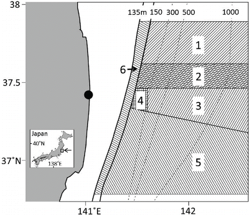
TABLE 1. Opening dates for trial bottom trawl fishing in the waters offshore of Fukushima, Japan. See Figure 1 for the location of each area.

Area	Opening date	Boundary depth (m)
1	Jun 18, 2012	150
2	Oct 19, 2012	150
3	Feb 18, 2013	150
4	May 24, 2013	150
5	Aug 28, 2013	150
6	Dec 25, 2013	135

The aim of this study was to develop a new surplus production model considering seasonal movements and different fishing pressures between two areas: the no-take area and the limited fishing area off Fukushima. The model was applied to Sea Raven populations off Fukushima by using CPUEs from 2000 to 2009 and was also used to predict the future biomass of Sea Ravens. We chose the Sea Raven as a suitable candidate because previous studies have reported that they exhibit clear seasonal movements from coastal to offshore areas in association with their reproductive cycles (Munehara 1996; Antonenko et al. 2010). The feasibility of the model was evaluated by comparing the predicted and observed CPUEs before (i.e., January 2010–March 2011) and after (i.e., September–October 2012) the nuclear accident at FDNPP based on data that were not included in the estimation step. Results of the model were used to evaluate whether the waters off Fukushima have been effectively serving as an MPA since the accident. We also demonstrate the model's applicability for estimating the optimum fishing effort and for designing a new MPA based on consideration of seasonal movements.

METHODS

Study area

The waters off Fukushima, where the cold Oyashio Current meets the warm Kuroshio Current (Shimizu et al. 2001), constitute a fertile fishing area. Many commercially important demersal fish stocks (e.g., Pacific Cod Gadus macrocephalus, Barfin Flounder Verasper moseri, Willowy Flounder Tanakius kitaharai, and Spotted Halibut Verasper variegatus) are distributed in this region and display some degree of seasonal movements between coastal and offshore areas (Narimatsu 2006; Narimatsu et al. 2007; Wada et al. 2012; Kayaba et al. 2014). Demersal fishes off Fukushima were fished by various commercial methods, such as gill-net fishing and bottom trawl fishing, prior to the FDNPP accident.

At the instruction of the Fukushima Prefectural Government, the Fukushima Fisheries Experimental Station has conducted monitoring surveys for radioactive iodine (¹³¹I) and Cs concentrations in Fukushima's marine products since April 7, 2011 (Wada et al. 2013). Whether or not fish can be landed via the trial fishing is determined based on the results of the monitoring surveys. The first trial fishing area was opened on June 18, 2012, and five other areas were opened sequentially thereafter (Figure 1; Table 1).

Data set used for analysis

Off Fukushima, 82.9% of the Sea Raven landings from 2000 to 2010 were caught by coastal gill-net fishing and offshore bottom trawl fishing. The waters off Fukushima were divided into coastal and offshore areas based on the operated depths of gill-net fishing and bottom trawl fishing. The location of each depth observation (Appendix, Figure A.1) was obtained from daily fishing logbooks. Some outliers or typographical errors were included in the logbooks; therefore, we removed the upper and lower 2.5th percentiles of the observed depth. The shallowest and greatest depths were calculated as 9.0 and 69.0 m for gill-net fishing and as 87.0 and 576.0 m for bottom trawl fishing. The average of the deepest observed gill net and the shallowest observed bottom trawl ([69.0 + 87.0]/2 = 78.0 m) was adopted as the boundary between gill-net and bottom trawl fishing areas. Here, we refer to areas shallower than 78.0-m depth as coastal areas, and we refer to waters deeper than 78.0 m as offshore areas. The fishing logbooks were recorded by a chief fisherman on each vessel and included data on fishing dates, depth, longitude, latitude, net deployment and net hauling times for each fishing operation, gill-net length and mesh size (for gill-net fishing), and maximum catch (nearest 0.1 kg) of 15 species for each operation. The number of vessels that cooperated to record the fishing logbooks differed among years. On average, 48 gill-net vessels (range = 44–52) and 11 bottom trawl vessels (range = 10–12) per year cooperated to record the logbook data during 2000–2010. The total number of registered vessels in Fukushima Prefecture was approximately 600 for gill-net fishing and approximately 40 for bottom trawl fishing, thus indicating that the cooperating vessels constituted 8.0% of all gill-net vessels and 27.5% of all bottom trawl vessels. Since the FDNPP accident, all bottom trawl vessels participating in the trial fishing operations have been recording logbook data. However, no data were available for gill-net fishing after the accident because there were no trial gill-net fishing operations for demersal fishes as of December 2014.

The tonnage of bottom trawl fishing vessels ranged from 17.0 to 47.6 metric tons, and the engine power of those vessels ranged from 502 to 670 kW. The reported cod-end mesh size used on the bottom trawl nets ranged from 5.0 to 9.0 cm, and the headrope length ranged from 28.3 to 37.4 m (Hirata 2000; Inoue and Honda 2002). Two types of otter boards were used: monoplane and biplane. The tonnage of gill-net fishing vessels ranged from 1.30 to 6.98 metric tons, and engine power ranged from 281 to 540 kW. The gill-net mesh size ranged from 9.59 to 16.7 cm, but the mean gill-net mesh size did not affect the monthly gill-net fishing CPUE (Figure A.2). Because there was little difference between observed and unobserved vessels, the vessels that cooperated to record the fishing logbooks were assumed to be representative of all gill-net and bottom trawl fishing vessels.

Monthly Sea Raven catch (C; metric tons/month) for all gill-net fishing and bottom trawl fishing from January 2000 to March 2011 was obtained from the annual report of fishery statistics in Fukushima (Fishery Office of the Fukushima Prefectural Government 2013). We obtained the logbook-recorded catch from the trial bottom trawl fishing that was conducted in September and October 2012. Effort from trial bottom trawling was obtained for June and September–December 2012. From 2000 to 2010, average catch per month was 1,020 kg (CV = 0.83) for gill-net fishing and 2,770 kg (CV = 0.98) for bottom trawl fishing. Total gill-net length per month and total bottom trawl towing hours per month as calculated from the fishing logbooks were used as the effort values (E). In other words, each monthly value of E was calculated from 8.0% of the gill-net vessels and 27.5% of the bottom trawl vessels, whereas data on monthly catch was from all of the vessels.

The total gill-net length or total bottom trawl towing hours were summed for each month. Because the unit of effort differed and data were obtained from different fishing gears, we transformed the monthly effort to values from zero to 1.0 by dividing by the monthly maximum effort values for 2000–2009 as follows:(1) (2) where s represents the shallow coastal fishing area (<78.0 m) for gill-net fishing and d represents the deep offshore area (≥78.0 m) for bottom trawl fishing. From the distribution of operated depth, we assumed that gill-net fishing was not carried out in the offshore fishing area and likewise that bottom trawl fishing did not occur in the coastal fishing area (Figure A.1), although at most 2.5% of the fishing activity by each vessel might involve crossing the boundary. The symbol t represents a cumulative month from 2000 to 2009; therefore, t = 1 represents January 2000 and t = 120 represents December 2009. The CPUEs of gill-net fishing (I_s) and bottom trawl fishing (I_d) were then calculated as(3) (4)

There was no effort in July and August for bottom trawl fishing, which was prohibited during those months. Records for depths greater than 314 m were excluded from the calculation because 314 m is the recorded deepest depth of the Sea Raven catch off Fukushima.

Population model

We developed a surplus production model that included a monthly rate of Sea Raven movement, X_m (−1 ≤ X_m ≤ 1), between the two fishing areas,(5) (6) (7) (8) where B^′ is biomass (metric tons) prior to movement, and m represents each month corresponding to t (i.e., m = 1 [January], … , 12 [December]). For example, X_m with t = 2 and t = 14 shows the same movement rate (X₂) in February 2000 and in February 2001. Sea Ravens move from the offshore area to the coastal area if X_m is larger than zero (equation 7(7) ); they will move from the coastal area to the offshore area if X_m is less than zero (equation 8(8) ). Estimated parameters include r (growth rate), K (carrying capacity in metric tons; K ≥ B), and q (fishing efficiency).

Observation model

We assumed that the natural logarithm of observed monthly CPUEs for gill-net fishing and bottom trawl fishing followed a normal distribution (N[μ, σ²]), with a mean value (μ) that was the natural logarithm of the estimated CPUE (log_e[q_sB_s] and log_e[q_dB_d]) from the model,(9) (10)

The variance (σ²) was assumed to be different for each gear ( and ).

Parameter estimation

The parameters were estimated by using the Markov chain–Monte Carlo method under the framework of Bayesian estimation. The software R version 3.1.0 (R Development Core Team 2014), the R package R2WinBUGS (Sturtz et al. 2005), and the Gibbs sampling program WinBUGS (Spiegelhalter et al. 2003) were used to estimate posterior distributions. The first 500,000 samples were not used due to the potential for them to be affected by initial values that were randomly selected from their prior distributions. The last 1,000,000 samples were used to obtain posterior distributions. Some parameters were sampled in the logarithmic scale to avoid cancellation of significant digits or to increase the efficiency of searching. Prior distributions of parameters were set as follows:(11)

In this case, the CPUEs from 2000 to 2009 were used to estimate the parameters. The developed model was evaluated by applying it to predict biomass before the nuclear disaster at FDNPP (January 2010–March 2011) and biomass after the disaster (September–October 2012).

Model evaluation and prediction of future biomass

By using estimated posterior distributions, we predicted future biomass of Sea Ravens from 2010 to 2015 under two scenarios. In scenario 1, the observed effort for each gear was continued at the same level as 2010. In scenario 2, the observed effort for each gear after the FDNPP accident was used (i.e., only the effort from the trial bottom trawl operation). In scenario 2, the predicted and observed CPUEs before the nuclear disaster (January 2010–March 2011) and after the disaster (September–October 2012) were compared to evaluate the predictive performance of the model. We randomly selected samples of each parameter from the posterior distributions, and future biomass from 2010 to 2015 was then predicted for each scenario. We repeated this prediction 10,000 times to calculate the median and 95% credible intervals for predicted biomass.

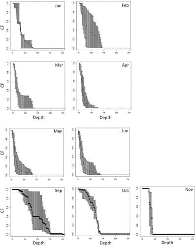
Although the developed model was able to estimate CPUE in the defined offshore area (q_dB_d[t]), it was unable to estimate the CPUE for the trial bottom trawl fishing area during 2012. Therefore, a corrected value of predicted biomass in the area deeper than 150 m was needed to compare the predicted and observed CPUEs from trial bottom trawl fishing. To correct the predicted biomass, we calculated a correction factor (CF) by using the monthly CPUEs from the daily bottom trawl fishing logbooks for 2000–2010. Generally, the CF provides good correction when CPUE is proportional to biomass,(12) where y represents the year (y = 2000, … , 2010); I_d,m,z is the CPUE of bottom trawl fishing that occurred deeper than depth z during month m; and I_d,m is the bottom trawl fishing CPUE calculated from all depth ranges greater than 78.0 m. This equation shows the ratio of CPUE equal to that of biomass. Therefore, CF_m,z is the ratio of biomass in the area deeper than 78.0 m and depth z during month m. The 95% confidence interval of CF_m,z was calculated by the bootstrap method. We randomly chose 11 years from 2000 to 2010 (with replacement) and calculated by using the hth bootstrap sample. This step was repeated 1,000 times (i.e., h = 1, … , 1,000), and the confidence interval of CF_m,z was calculated.

For the evaluation step, mean CF_m,150 was multiplied by the corresponding monthly predicted biomass. The corrected predicted biomass in the area deeper than 150 m (B_d[t]CF_m,150) was then obtained and used to predict CPUE for September and October 2012. The value of CF_m,z was also used to examine the effect of a simulated MPA (see below).

Estimating the optimum fishing effort

Two different simulations were carried out to estimate the optimum levels of effort for gill-net fishing and bottom trawl fishing and to show the effects of an MPA. The period of simulations was set at 100 years, which was long enough to confirm whether predicted catch and biomass (see equations 13–17 and equation 20(20) below) decreased if effort was too high. For simplicity, effort for each gear type was fixed through time (i.e., = ; and = ), and the estimated median values of the parameters were used in calculations.

First, we simulated future biomass to investigate the optimal fishing effort for maximizing total catch by varying the levels of gill-net fishing effort and bottom trawl fishing effort from 0 to 1. We calculated a predicted total catch for 100 years (TC) and the predicted biomass 100 years later (PB) as(13) (14) (15) (16) where t = 133 represents January 2011; t = 1321 represents January 2111; and t = 1332 represents December 2111. The mean gill-net fishing effort () and the mean bottom trawl fishing effort () before the nuclear disaster were calculated as follows:(17) (18)

The gill-net effort and bottom trawl effort that maximized the value of TC_s + TC_d were defined as the optimal effort levels, and the ME^′ values before the disaster were compared.

Estimating the effects of a simulated marine protected area

We also calculated the total catch and biomass by varying the boundary depth and . The boundary depth determines the area where trial bottom trawl fishing can occur. In other words, a change in the boundary depth is equivalent to a change in the size of an MPA. We used the mean CF_m,z to simulate the trial fishing catch in the area deeper than the boundary depth z as(19) where B_d(t)CF_m,z is the corrected biomass in the area deeper than depth z (i.e., biomass outside of the MPA) and C_d,z is the expected catch for bottom trawl fishing conducted in that area. In this simulation, the range of was set at 0 to 5, and the boundary depth was set at 78.0 to 180 m. The gill-net fishing effort was set at zero through time. We calculated the total catch in the area deeper than the boundary depth z (TC_d,z) by using C_d,z as follows:(20)

RESULTS

The natural logarithms of estimated monthly CPUEs for both gill-net fishing and bottom trawl fishing are shown in Figure 2a and 2b, respectively. Almost all of the observed CPUEs for gill-net fishing (93.3%) and bottom trawl fishing (97.0%) were included within the 95% credible intervals of the estimated CPUEs. The estimated cyclic variation in CPUE was consistent with the cyclic variation in estimated Sea Raven biomass. The medians of the posterior distribution of biomass at each time point changed cyclically between the coastal and offshore areas (Figure 3). When biomass in the offshore area was high, biomass in the coastal area was low (e.g., in September) and vice versa (e.g., in December).

FIGURE 2. Estimated median CPUEs (solid line; log_e transformed) and 95% credible intervals (dotted lines) for Sea Ravens captured by (a) gill-net fishing and (b) bottom trawl fishing off Fukushima, Japan (open circles = observed monthly CPUEs; black circles = CPUEs observed in January of each year). There are no CPUEs for bottom trawl fishing in July or August because bottom trawling was prohibited during those months.

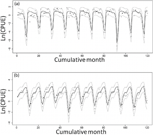
FIGURE 3. Estimated median biomass of Sea Ravens (metric tons) obtained from the model developed in this study. Biomass in the coastal area (<78.0 m; dotted line) and biomass in the offshore area (≥78.0 m; solid line) are depicted (open circles = monthly biomass; black circles = biomass in January of each year).

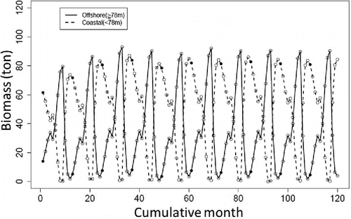
Monthly movement rates (Figure 4) reflected the spatiotemporal variation in Sea Raven biomass between the coastal and offshore areas. The estimated posterior distributions of movement rate showed that Sea Ravens stayed in the coastal area from approximately January through April (Figure 4). The fish then started to move from the coastal area to the offshore area from May to August. In September, Sea Ravens began to move back into the coastal area from the offshore area. Medians and 95% credible intervals for the other parameters are shown in Figure 5a–g and Table 2.

FIGURE 4. Estimated posterior distributions of Sea Raven movement rates off Fukushima (black circle = median; ±95% credible interval). Positive values indicate fish movement from the offshore area to the coastal area; negative values indicate movement from the coastal area to the offshore area.

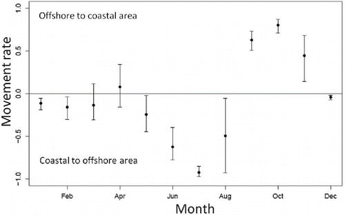
FIGURE 5. Histograms of estimated posterior distributions for the natural logarithms of (a) Sea Raven intrinsic growth rate (r); (b) gill-net fishing efficiency (q_s); (c) bottom trawl fishing efficiency (q_d); (d) carrying capacity of the coastal area (<78.0 m; K_s); (e) carrying capacity of the offshore area (≥78.0 m; K_d); (f) biomass for the coastal area in January 2000 (B_s[1]); (g) biomass for the offshore area in January 2000 (B_d[1]). Dotted lines indicate the prior distributions.

TABLE 2. Estimated median, 2.5% quantile, and 97.5% quantile of the posterior distributions for each parameter (subscript s represents the shallow coastal fishing area [<78.0 m] for gill-net fishing; subscript d represents the deep offshore area [≥78.0 m] for bottom trawl fishing; r = growth rate; q = fishing efficiency; K = carrying capacity; B[1] = biomass in January 2000).

Parameter	2.5%	Median	97.5%
loge(r)	−3.40	−2.74	−1.94
loge(qs)	−3.93	−3.46	−2.97
loge(qd)	−2.26	−1.77	−1.35
loge(Ks)	4.31	5.48	9.74
loge(Kd)	4.41	6.23	9.77
loge(Bs[1])	3.35	4.07	4.68
loge(Bd[1])	1.65	2.54	3.42

The median of the average yearly biomass (i.e., the mean monthly biomass from January to December) calculated for scenario 1 was smaller than that for scenario 2 in both the coastal area and the offshore area (Figure 6). This result indicates that Sea Raven biomass will increase in the no-take area and in the trial fishing area off Fukushima if fishing effort only occurs at the trial levels.

FIGURE 6. Medians (±95% credible interval) of the average predicted Sea Raven biomass (log_e transformed) per year in the coastal area (squares) and offshore area (circles; open symbols = scenario 1, in which the observed effort for gill-net fishing and bottom trawling was continued at the same levels as 2010; shaded symbols = scenario 2, in which the observed effort after the FDNPP accident was used [i.e., trial bottom trawl fishing only]).

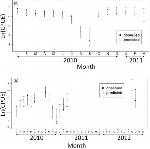
Almost all of the observed monthly CPUEs for gill-net fishing (86.7%) and bottom trawl fishing (73.3%) were included in the 95% credible intervals of predicted CPUEs (Figure 7). During 2012, catch of Sea Ravens was only recorded in September and October, consistent with the result that the fish were mainly distributed in the offshore area during those months (Figure 3).

FIGURE 7. Medians of the predicted CPUE (open circles; log_e transformed, ±95% credible interval) and observed CPUE (black circles; log_e transformed) for Sea Ravens captured by (a) gill-net fishing (January 2010–March 2011) and (b) bottom trawl fishing (January 2010–October 2012).

Estimated Optimum Fishing Effort to Maximize the Total Catch

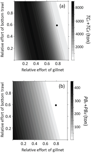
The sum of TC_s and TC_d was maximized at 8,090 metric tons when was 0.20 and when was 1.00 (Figure 8a). The calculated and were 0.79 and 0.59, respectively, with a summed TC of 904 metric tons. This indicates that the mean gill-net fishing effort was too high and that 7,186 metric tons would be lost during this period. The sum of PB_s and PB_d was 1.13 metric tons when the mean effort levels ( and ) were continued, whereas the optimized effort values yielded a summed PB of 330 metric tons (Figure 8b). Sea Raven catch and biomass both increased under the optimized levels of gill-net and bottom trawl fishing effort compared with the mean fishing effort levels that were observed before the disaster.

FIGURE 8. Sum of (a) the predicted total Sea Raven catch (metric tons) for 100 years of gill-net fishing (TC_s) and bottom trawl fishing (TC_d) and (b) the predicted Sea Raven biomass (metric tons) 100 years later (2111) in the coastal area (PB_s) and offshore area (PB_d) off Fukushima, Japan. The x- and y-axes show the gill-net fishing effort () and bottom trawl fishing effort (). The black circle indicates the mean gill-net fishing effort () or mean bottom trawl fishing effort () before the nuclear disaster.

Effects of the Boundary Depth on Total Catch and Biomass

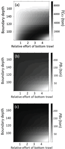
The calculated mean CF_m,z is shown in Figure 9, and the confidence intervals of mean CF_m,z as calculated by the bootstrap method are presented in Figure A.3. In some cases, the calculated TC_d,z decreased when was high (Figure 10a). For example, the maximum TC_d,z was 8,071 metric tons when (1) PB_s and PB_d were 98.2 and 119 metric tons, respectively; (2) the boundary depth was set at 78.0 m; and (3) was set at 2.20 (Figure 10a–c). However, TC_d,z decreased and Sea Raven biomass approached zero when was greater than 2.20. The sum of PB_s and PB_d was 332 metric tons when was set at 1.0, the maximum effort of bottom trawl fishing. This was greater than the mean biomass for the period 2000–2009 (85.6 metric tons).

FIGURE 9. Calculated mean value of the correction factor (CF_m,z) for each month from 2000 to 2010 (see Methods). Note that there was no CF for July or August because bottom trawl fishing was prohibited during those months. There was no CF for December because Sea Ravens were not recorded in the fishing logbooks for December of 2000–2010.

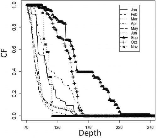
FIGURE 10. (a) Predicted total catch (metric tons) of Sea Ravens by bottom trawl fishing for 100 years (TC_d,z) with different boundary depths; (b) predicted Sea Raven biomass (metric tons) 100 years later in the coastal area (PB_s); and (c) predicted biomass 100 years later in the offshore area (PB_d). The x-axis shows the bottom trawl fishing effort ().

DISCUSSION

Waters off Fukushima as an Effective Marine Protected Area

We demonstrated that spatiotemporal changes in Sea Raven biomass caused by seasonal movements and different fishing pressures between the two areas can be estimated using the developed surplus production model. In addition, biomass after the FDNPP accident can be predicted with this model. The results suggest that the predicted Sea Raven biomass in the coastal and offshore areas increased when fishing effort remained at levels occurring since the FDNPP accident (Figure 6). Moreover, the high predictive ability of the model was demonstrated by the fact that almost all of the observed CPUE values were within the 95% confidence intervals of the predicted CPUEs (Figure 7).

Results showed that the sum of PB_s and PB_d was larger than the mean biomass before the disaster when was set at 1.0 and when boundary depth was set at 78.0 m (Figure 10). This finding indicates that Sea Raven biomass will increase and that the waters off Fukushima can serve as an effective MPA for Sea Ravens even if the bottom trawl fishing area and effort are completely restored.

A recent study proposed five key features of a successful MPA: no take, well enforced, old (>10 years), large size (>100 km²), and isolated from fishing areas by deep water or sand (Edgar et al. 2014). Under its current status, the Fukushima coast has at least two of those key features (well enforced and large), and the coastal area is a no-take zone. Our present results support the area's potential to be a successful MPA. The mean CPUE of exploited species from the trial fishing in 2012 was about three times the mean CPUE per year from 2007 to 2009 (Yamada et al. 2014), indicating that the effective MPA has not only influenced Sea Raven biomass but also the biomass levels of other commercial species.

General Applications of the Model

The model developed here is not limited to biomass estimation between a no-take area and a fishing area; it is also useful for estimating optimal fishing pressure under a stock management strategy by varying the gear-specific effort levels, as we have shown. By applying our model to other exploited species, we could simulate various fishery management strategy scenarios. For example, the model may be applicable in estimating biomass and optimal fishing pressure in cases where the seasonal migration of a stock occurs inside and outside of the exclusive economic zone.

Furthermore, our model will be useful in evaluating the effect of an MPA on catch and biomass before MPA establishment if data on CPUEs at the candidate site and surrounding fishing areas are available. In fact, we used our model to show the expected catch and biomass in a simulated MPA (Figure 10). However, at least a one-dimensional relative spatial distribution of the target species is needed to estimate the effect of different MPA sizes. Although we used a CF to obtain the relative spatial distribution of Sea Ravens (Figure 9) against a certain depth, depth-specific CPUEs are usually difficult to obtain. A statistical model (e.g., a generalized linear model [GLM]) for estimating spatial distribution (Guisan and Thuiller 2005) would be useful if related covariates are available as explanatory variables.

Required Data and Model Assumptions

The model we developed is applicable to species that move between two areas if spatiotemporal CPUEs are available from both areas. Although we used monthly CPUEs, the temporal and spatial scales can be changed to match a migrating type of target species.

The efficiencies of gill-net fishing and bottom trawl fishing were estimated from the developed model. Some researchers may standardize CPUEs so as to estimate the difference in efficiency between gill-net and bottom trawl fishing with a GLM. Estimated efficiencies from GLMs are usually relative efficiencies among gears (e.g., Campbell 2004); however, our model gave estimates of absolute efficiency when the unit of effort and biomass was given. Moreover, although both types of model can estimate the effect of gear on CPUE, the present model was able to estimate the incremental effect of gill-net fishing effort on the CPUE of bottom trawl fishing and vice versa. In terms of effort control for stock management, the model we developed is useful.

We used separate values of K for the coastal area and the offshore area because coastal waters usually display higher productivity than offshore waters. Moreover, the two study areas differed in size. If there are no environmental differences between two areas, setting a single K-value in the model and allocating it to the areas based on the ratio of their sizes might be useful for reducing the number of parameters.

The posterior distribution of K had longer tails than the distributions of the other parameters (Figure 5). In a previous study, Hilborn and Walters (1992) reported that a CPUE determined under conditions of high biomass and low fishing effort is necessary for the estimation of K. However, the mean gill-net fishing effort before the FDNPP disaster was more than four times the optimal effort. This might explain why the posterior distribution of K had long tails.

Although conventional tagging data have been widely used to examine population size and mortality, exploitation, growth, and movement rates in fisheries (Kurota et al. 2009), two assumptions must be met: (1) the reporting rate must be known and (2) fish behavior must not be impacted by tagging (Sibert et al. 1999; Pine et al. 2003). Our study suggests that given a sufficient contrast in CPUE between two areas, tagging is not required to estimate biomass, fishing efficiency, growth, movement rate, and K. Eliminating the need for tagging data is one advantage of the present model, which is easily implemented for new data sets.

Conclusions

Our model predicted that Sea Raven biomass off Fukushima will increase in the future if fishing effort is kept at trial levels. The results revealed that the waters off Fukushima have effectively acted as an MPA since the FDNPP accident. This model will also be useful for other studies of migrating species—for example, to estimate the optimal fishing pressure for a stock that migrates seasonally within and outside of the exclusive economic zone or to evaluate effects on biomass at a candidate site before its establishment as a new MPA.

ACKNOWLEDGMENTS

We are grateful to all those who contributed to data collection. We thank Hiroyuki Matsuda, Takashi Matsuishi, Miyako Naya, and two anonymous reviewers for useful comments on a draft of the manuscript. This work was supported by a Grant-in-Aid (25082C) from the Agriculture, Forestry, and Fisheries Research Council to T.M.

Appendix: Additional Data

FIGURE A.1. Density distributions of gill-net operation depth (dotted line) and bottom trawl operation depth (solid line) in the waters off Fukushima, Japan, from 2000 to 2010 based on information from daily fishing logbooks (with outliers and typographical errors removed).

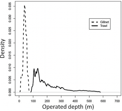
FIGURE A.2. Relationship between the monthly gill-net fishing CPUE values included in our analysis and the mean gill-net mesh size used during each month from 2000 to 2010 (correlation coefficient r = 0.043; P = 0.636).

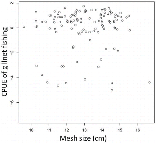
FIGURE A.3. Bootstrapped averages (with 95% confidence interval) of correction factors (CF_m,z) for each month. Note that there were no CF_m,z values for July or August because bottom trawl fishing was prohibited during those months. There was no CF_m,z in December because Sea Ravens were not recorded in the fishing logbooks for December of 2000–2010.

REFERENCES

- Agardy, T. M. 1994. Advances in marine conservation: the role of marine protected areas. Trends in Ecology and Evolution 9:267–270.
- Allison, G. W., J. Lubchenco, and M. H. Carr. 1998. Marine reserves are necessary but not sufficient for marine conservation. Ecological Applications 8(Supplement):S79–S92.
- Antonenko, D., O. Pushchina, S. Solomatov, and P. Kalchugin. 2010. Distribution and some features of biology of Sea Raven Hemitripterus villosus (Hemitripteridae) in the northwestern part of the Sea of Japan. Journal of Ichthyology 50:640–649.
- Campbell, R. A. 2004. CPUE Standardisation and the construction of indices of stock abundance in a spatially varying fishery using general linear models. Fisheries Research 70:209–227.
- Coggins, L. G. Jr., W. E. Pine III, C. J. Walters, and S. J. Martell. 2006. Age-structured mark–recapture analysis: a virtual-population-analysis-based model for analyzing age-structured capture–recapture data. North American Journal of Fisheries Management 26:201–205.
- Edgar, G. J., R. D. Stuart-Smith, T. J. Willis, S. Kininmonth, S. C. Baker, S. Banks, N. S. Barrett, M. A. Becerro, A. T. Bernard, and J. Berkhout. 2014. Global conservation outcomes depend on marine protected areas with five key features. Nature 506:216–220.
- Field, J. C., A. E. Punt, R. D. Methot, and C. J. Thomson. 2006. Does MPA mean “major problem for assessments”? Considering the consequences of place-based management systems. Fish and Fisheries 7:284–302.
- Fishery Office of the Fukushima Prefectural Government. 2013. Annual report of fishery statistics in Fukushima. Available: http://www.pref.fukushima.lg.jp/sec/36035e/suisanka-toukei-top.html. (July 2015.) (In Japanese.)
- Guénette, S., T. Lauck, and C. Clark. 1998. Marine reserves: from Beverton and Holt to the present. Reviews in Fish Biology and Fisheries 8:251–272.
- Guisan, A., and W. Thuiller. 2005. Predicting species distribution: offering more than simple habitat models. Ecology Letters 8:993–1009.
- Halpern, B. S., and R. R. Warner. 2002. Marine reserves have rapid and lasting effects. Ecology Letters 5:361–366.
- Hart, D. R. 2006. When do marine reserves increase fishery yield? Canadian Journal of Fisheries and Aquatic Sciences 63:1445–1449.
- Hilborn, R., and C. J. Walters. 1992. Quantitative fisheries stock assessment: choice, dynamics and uncertainty. Springer, New York.
- Hirata, T. 2000. Structure of existing offshore trawl in the Soma Haragama region of Fukushima Prefecture. Bulletin of the Fukushima Prefecture Fisheries Experiment Station 9:83–89. (In Japanese.)
- Holland, D. S. 2002. Integrating marine protected areas into models for fishery assessment and management. Natural Resource Modeling 15:369–386.
- Inoue, Y., and T. Honda. 2002. Haragama design of coastal selective trawl net (HD-STN). Technical Report of the National Research Institute of Fisheries Engineering 24:27–30. (In Japanese.)
- Jones, P. J. 2001. Marine protected area strategies: issues, divergences and the search for middle ground. Reviews in Fish Biology and Fisheries 11:197–216.
- Kayaba, T., T. Wada, K. Kamiyama, O. Murakami, H. Yoshida, S. Sawaguchi, T. Ichikawa, Y. Fujinami, and S. Fukuda. 2014. Gonadal maturation and spawning migration of stocked female Barfin Flounder Verasper moseri off the Pacific coast of northern Japan. Fisheries Science 80:735–748.
- Kurota, H., M. K. McAllister, G. L. Lawson, J. I. Nogueira, S. L. Teo, and B. A. Block. 2009. A sequential Bayesian methodology to estimate movement and exploitation rates using electronic and conventional tag data: application to Atlantic Bluefin Tuna (Thunnus thynnus). Canadian Journal of Fisheries and Aquatic Sciences 66:321–342.
- Lester, S. E., B. S. Halpern, K. Grorud-Colvert, J. Lubchenco, B. I. Ruttenberg, S. D. Gaines, S. Airamé, and R. R. Warner. 2009. Biological effects within no-take marine reserves: a global synthesis. Marine Ecology Progress Series 384:33–46.
- Munehara, H. 1996. Sperm transfer during copulation in the marine sculpin Hemitripterus villosus (Pisces: Scorpaeniformes) by means of a retractable genital duct and ovarian secretion in females. Copeia 1996:452–454.
- Narimatsu, Y. 2006. Reproductive biology of Pacific Cod, a review especially referring to interannual variations of biomass, age and size at maturity and fecundity. Bulletin of the Fisheries Research Agency 4:137–146. (In Japanese.)
- Narimatsu, Y., A. Yamanobe, and M. Takahashi. 2007. Reproductive cycle, age, and body size at maturity and fecundity of female Willowy Flounder Tanakius kitaharai. Fisheries Science 73:55–62.
- Pincin, J. S., and M. J. Wilberg. 2012. Surplus production model accuracy in populations affected by a no-take marine protected area. Marine and Coastal Fisheries: Dynamics, Management, and Ecosystem Science [online serial] 4:511–525.
- Pine, W. E., K. H. Pollock, J. E. Hightower, T. J. Kwak, and J. A. Rice. 2003. A review of tagging methods for estimating fish population size and components of mortality. Fisheries 28(10):10–23.
- Punt, A. E., and R. D. Methot. 2004. Effects of marine protected areas on the assessment of marine fisheries. Pages 133–154 in S. J. Brooke, editors. Aquatic protected areas as fisheries management tools. American Fisheries Society, Symposium 42, Bethesda, Maryland.
- R Development Core Team. 2014. R: a language and environment for statistical computing. R Foundation for Statistical Computing, Vienna.
- Shimizu, Y., I. Yasuda, and S. Ito. 2001. Distribution and circulation of the coastal Oyashio intrusion. Journal of Physical Oceanography 31:1561–1578.
- Sibert, J. R., J. Hampton, D. A. Fournier, and P. J. Bills. 1999. An advection–diffusion–reaction model for the estimation of fish movement parameters from tagging data, with application to Skipjack Tuna (Katsuwonus pelamis). Canadian Journal of Fisheries and Aquatic Sciences 56:925–938.
- Spiegelhalter, D., A. Thomas, N. Best, and D. Lunn. 2003. WinBUGS users' manual. Medical Research Council, Biostatistics Unit, Cambridge, UK.
- Sturtz, S., U. Ligges, and A. E. Gelman. 2005. R2WinBUGS: a package for running WinBUGS from R. Journal of Statistical Software [online serial] 12(3).
- Wada, T., K. Kamiyama, S. Shimamura, T. Mizuno, and Y. Nemoto. 2012. Effectiveness of stock enhancement of a rare species, Spotted Halibut Verasper variegatus, in Fukushima, Japan. Aquaculture 364/365:230–239.
- Wada, T., Y. Nemoto, S. Shimamura, T. Fujita, T. Mizuno, T. Sohtome, K. Kamiyama, T. Morita, and S. Igarashi. 2013. Effects of the nuclear disaster on marine products in Fukushima. Journal of Environmental Radioactivity 124:246–254.
- Yamada, M., T. Sohtome, and T. Iwasaki. 2014. Comparisons of fishing efforts and fishery resource abundance off Fukushima before and after the Great East Japan Earthquake. Tohoku Demersal Fish Research 34:63–66. (In Japanese.)