Multi-depot bus schedule assignment with parking and maintenance constraints for intercity transportation over a planning period

ABSTRACT

This article introduces the schedule assignment problem for public transit, which aims to assign vehicle blocks of a planning period to buses in the fleet of a transportation company. This assignment has to satisfy several constraints, the most important of which is compatibility, meaning that certain blocks can only be serviced by buses belonging to given types. Other constraints come from the fact that the problem considers a long-term plan for several days or weeks, which means that daily parking and periodic maintenance activities also have to be taken into account. We give a state-expanded multi-commodity flow network for the above problem. This model takes parking constraints into account, and also assigns preventive maintenance tasks to buses after serving blocks for a fixed amount of time. The solutions of this model are presented for real-life and randomly generated instances.

KEYWORDS:

• Bus scheduling
• parking
• maintenance
• long-term planning
• public transportation
• assignment
• integer programming
• network flow

Introduction

Creating a long-term schedule is one of the most important optimization problems of a transportation company. This usually considers a planning period of several days or weeks, with timetabled tasks that have to be serviced every day. When such a schedule is created, the timetabled trips that should be carried out by the same vehicles are organized into different vehicle blocks, which form the daily vehicle schedule together. As a result, these blocks can be considered as sequences of tasks that the vehicles of the company have to execute on the given day. An important feature of the problem is that the days of this planning period are generally not completely independent of each other, and they can be divided into different day-types, such as workdays and holidays. Days that share a day-type have the same underlying timetable of trips, and the same daily schedule can be applied to them because of this.

Vehicle blocks will be the same for every day that share the same day-type. However, the vehicles executing these blocks might be different on two separate days. A daily vehicle schedule can be created by solving the vehicle scheduling problem (VSP), which is a well studied field in the literature. This problem receives the timetabled trips of the company as an input, and creates assigns sequences of these trips to theoretical vehicles in the fleet of the company, creating vehicle blocks during the process.

Yet, the assignment of real vehicles to these blocks over a longer horizon is not really considered to our knowledge, and even less attention is given to intercity transportation. The aim of this article is to propose a long-term assignment between the daily vehicle blocks and the fleet of a transportation company that satisfies arising constraint such as parking and maintenance. Such constraints are especially important in the case of intercity transportation. While vehicles performing urban schedules usually end their day in the same garage where they started, buses in intercity transportation might finish their daily tasks at garages that are different from their starting locations. Traveling to these places can mean significant extra costs for the company, and minimizing such travel costs are crucial to their expenses. Moreover, dealing with the theory of intercity bus transportation is especially important nowadays: a recent review on the quality of public transportation by Ojo (2017) states that intercity bus transportation plays a major part in commuting and long-distance movement.

While the goal of the problem is to give an assignment for every day of the planning horizon, this should not be done sequentially on a day-by-day basis, as the optimal solution is most likely lost in the process. The assignment of every vehicle and task has a global effect on other days of the horizon as well, and all constraints for every day should be considered together because of this.

The outline of the article is the following: first, we present the problems of vehicle scheduling and maintenance, and give a literature overview of these topics. Using the introduced concepts, we define the schedule assignment problem, which aims to assign daily blocks to vehicles of the company over a planning period, with respect to parking and maintenance constraints. We introduce a state-expanded multi-commodity flow network for this problem. The mathematical model of this network is solved using a mixed-integer programming (MIP) solver, and its results are presented both for real-life and randomly generated instances. Our preliminary results on this topic can be seen in the extended conference abstract Dávid (2016).

Scheduling vehicle tasks and maintenance activities

Creating a vehicle schedule for a single day is known in literature as the VSP. The schedule given by the VSP is made up of blocks, a block being the sequence of tasks serviced by a single vehicle for that day. For the introduction of the VSP, we refer to our formalization in Dávid and Krész (2017).

The input of the problem is the set $V$ of vehicles and $T$ of service trips. The features of these trips include a departure and arrival time, a starting and ending location, and a covered distance. A $(t,t^{\prime })$ pair of trips are compatible, if the same vehicle can service both trips; the arrival time of $t$ has to be lower than the departure time of $t^{\prime }$, and if the starting location of $t^{\prime }$ is different from the ending location of $t$, then the vehicle must be able to execute a so-called deadhead trip between these two locations.

The VSP assigns the trips of the given timetable to vehicles, satisfying the following conditions:

• Every trip in $T$ must be executed exactly once.

• For every $v\in V$, the trips assigned to $v$ must be compatible with each other.

• The cost of the assignment must be minimal. The solution of the VSP has two main cost components: a cost proportional to the distance traveled by the vehicles, and a one-time cost given by each vehicle that is used in the solution.

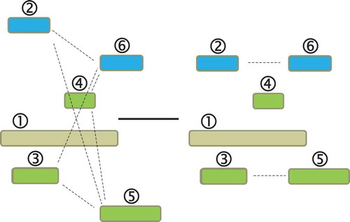
The problem is illustrated in Figure 1. The five trips of the input are represented by the boxes on the left, and trip compatibilities are given by the dashed lines. The right part of the figure shows a possible solution with four vehicle blocks.

Figure 1. Creating vehicle blocks from trips (taken from Árgilán et al. (2014)).

A set $D$ of depots can also be introduced for the problem. In this case, every $v\in V$ vehicle has a depot-type $d(v)\in D$. Vehicles having the same depot-type share the same characteristics, and also have the same costs. If a vehicle $v$ belonging to depot $d$ is used in the solution, it contributes a cost of $dc(d)+tc(d)\cdot dist(v)$, where $dc(d)$ is the one-time daily cost, and $tc(d)$ is the cost of traveling a unit distance for a vehicle belonging to depot $d$, while $dist(v)$ is the distance covered by vehicle $v$ in the solution. While the concept of depots traditionally separates vehicles that start the planning period at the same geographical location, these groups can easily be extended to consider vehicle characteristics (vehicle types) as well. In this article, a depot will include vehicles that start the planning horizon at the same geographical location, and also have the exact same characteristics. A binary depot-compatibility vector ${\mathbf{v}}^{\mathbf{t}}=(v_1,...,v_{\left|D\right|})$ can also be introduced for every trip $t\in T$. If such a vector exists, a vehicle belonging to depot $d$ can only service trip $t$, if $v_d^t=1$.

If the problem has only one depot, it is called a single depot vehicle scheduling problem (SDVSP), and can be solved in polynomial time. A formulation for the SDVSP can be seen in Bodin and Golden (1981). If the number of depots is at least two, we get a multiple depot vehicle scheduling problem (MDVSP). The MDVSP was introduced in Bodin et al. (1983) and is proven to be NP-hard by Bertossi, Carraresi, and Gallo (1987). Several different models have been proposed for the representation of the problem over the years, including but not limited to a decomposition (Saha (1970)), assignment (Orloff (1976)), and flow (Bodin et al. (1983)) models. An overview of research on the VSP can be found in Bunte and Kliewer (2009).

The result given by the above VSP corresponds to a set of vehicle blocks for one day. A vehicle block gives the tasks that a single vehicle has to execute on the given day, and also specifies the type of vehicle that can execute it. However, the VSP does not assign specific vehicles to its blocks, and because of this, the result can be called a ‘theoretical’ schedule, as further steps have to be taken to determine the exact vehicles in service on the current day.

When the concept of a heterogeneous vehicle fleet is important, a multi-vehicle type scheduling problem (MVTSP) can also be considered. This problem is frequently treated as an alternative version of the MDVSP, as mentioned before. However, several papers have studied problems with multiple vehicle types in the past years. While Laurent and Hao (2009) study the problem as a variant of the MDVSP, and give a powerful iterated local search method for its solution, Ceder (2011) emphasizes the concept of multiple vehicle types, and uses a so-called deficit function (DF) approach to visualize the number of particular vehicles at each location in the system. A column generation-based solution framework was proposed for the MVTSP by Guedes and Borenstein (2015).

Literature on vehicle scheduling over a planning period is really scarce, publications usually focus on creating optimal schedule for a single day. Papers dealing with a longer horizon usually study rolling stock rotations, vehicle maintenance, or try to integrate driver rostering with vehicle assignment.

Integrated vehicle assignment and driver rostering

Driver rostering aims to assign duties to the workers of the company over a planning horizon under different constraints. While this is a separate research field in itself (see Ernst et al. (2004) for a review), there are certain papers dealing with the integration of vehicle assignment.

Peters, de Matta, and Boe (2007) gave a branch-and-price framework for the problem aided by a GRASP, and presented their results of both real and simulated data. They consider both a primary and secondary job type for the drivers, and address a fleet of heterogeneous vehicles. This problem formulation is further studied in de Matta and Peters (2009), where they present the set covering mathematical model behind the framework.

The vehicle-crew rostering problem (VCRP) is proposed by Mesquita et al. (2011), where they aim to give an assignment between trips, duties, drivers, and buses. They propose a preemptive goal programming heuristic, which decomposes the VCRP into daily problems, and joins their outputs to create the final roster.

Sargut, Altuntas, and Tulazoğlu (2017) consider a multi-objective crew rostering problem, and proposes a model with assignment variables between vehicles and blocks. A tabu search method is proposed for the solution of the problem, and results are presented on smaller instances.

Rolling stock rotations

Papers about rotation planning aim to optimize long-distance railway transportation, creating cyclic plans based on a standard week using timetabled trips. Borndörfer et al. (2015) present a hypergraph-based MIP model for the rolling stock rotation planning problem for intercity railway. They consider railway vehicle compositions, and also include maintenance constraints and infrastructure capacities, and focus on the cyclic planning period of a standard week. This model was first studied in Borndörfer et al. (2011, 2012). Their results are presented on use-case scenarios of the Deutsche Bahn.

Integrating maintenance into the rolling stock circulation problem is also studied by Giacco, D’Ariano, and Pacciarelli (2014). They consider the same timetable to be repeated every day (calling it a cyclic timetable), with scheduled train services also given in the input. Their proposed model inserts the maintenance activities into this pre-determined assignment, and aims to produce a cyclic roster where the number of days is minimal. In Giacco et al. (2014), they describe a framework that sequentially creates rolling stock rosters, then assign maintenance to those using the above approach. Their results are presented on small scenarios of an Italian railway company.

Lai, Fan, and Huang (2015) consider a MIP and a hybrid heuristic model for the rolling stock assignment with maintenance constraints. They examine a single day, which is further divided into two time slots. The assignment of a longer period is done sequentially over these time slots. They conduct optimization on a daily basis, and only consider a look-ahead of 4 days when making decisions. A rolling horizon is used with the above sequential solution approach to give results for a 90-day period.

Bus transportation and maintenance

To our knowledge, the maintenance scheduling problem for buses is only studied by Haghani and Shafahi (2002). They examine the insertion of different maintenance activities into existing bus schedules over several days, but the assignment of schedules to buses is given in the input. They formulate multiple mathematical models for the assignment of maintenance task into time slots of the pre-determined schedules of the buses, and give test results for two different sets; a smaller example, where maintenance is scheduled for a vehicle fleet of 10 buses over a 3-day planning period, and a larger example of 181 buses and 182 days. However, they run the scheduling simulation daily in the latter case, and solve single problems sequentially for each day.

Our preliminary work in Dávid (2016) considered the problem of schedule assignment with parking constraints only. A sequential heuristic was proposed for the problem, and its results were evaluated with the help of a MIP model.

Our contribution

Our motivation behind developing the schedule assignment problem was the introduction of a model which creates a rostering over a longer planning period (several weeks, not just days), where:

• Every daily block is assigned to the buses in the fleet of the company.

• Buses are also sent to garages at the end of every day.

• Regular preventive maintenance activities are carried out for every bus.

• And all of the above constraints are optimized together, minimizing the arising travel and operational costs.

Although all the above requirements were studied before (see Subsections 2.1, 2.2, and 2.3), they either have not been considered together in the same problem, or solutions for a longer period were acquired by a sequential solution of smaller subproblems of days. Considering a longer planning period, both approaches have the same issue: the decisions made when fulfilling a requirement, or developing a daily solution do not only have a local effect on the given day but also affect the entire horizon.

Because of this, all constraints for every day should be considered in the same problem, otherwise the optimal, or good quality solutions might be lost in the solution process. Our goal is to give a model that represents the structure of the entire problem, and optimizes the whole horizon at once, considering all arising constraints together.

As the model is capable of providing solutions for a period of multiple weeks, its results can be used in a decision support system to aid long-term planning. Different configurations of vehicle fleet, maintenance and garage capacities and block types can be experimented with, and the resulting possible feasible solutions can help experts of the company in making a decision about the final schedule.

Schedule assignment problem

As seen in Section 2, the resulting schedules of the VSP only give the vehicle blocks for a single day. This alone, however, is not enough, as transportation companies create their schedules in advance for a planning period (e.g. several weeks, or even months). The days of this planning period are usually divided into different ‘day-types’ (workday, Saturday, holiday, etc.), and a theoretical vehicle schedule is created for each of these. This means that days belonging to the same day-type will have the exact same vehicle blocks, and same blocks will always have the same vehicle requirements throughout the entire planning period. However, they will not necessarily be executed by the same vehicle on different days.

The input for the schedule assignment problem is the $n$-day planning period of the company, with each day $i$ having an assigned day-type $dt(i)$. The set $V$ of vehicles available over the planning period is given as well. A set $D$ of depots is also introduced for these vehicles, and the depot-type $d(v)\in D$ is determined for every $v\in V$. Similarly to the VSP, vehicles belonging to the same depot share the same costs and characteristics. Set $G$ represents garages where vehicles can stay for the night between two days of the planning period.

A theoretical vehicle schedule is also provided for every day-type $dt(i)$, which is the set $S(dt(i))$ of vehicle blocks that have to be executed on days of the given type. We consider these schedules (and also the blocks contained by them) theoretical, because they only give the sequences of timetabled tasks that have to be executed on days of the given type. However, they do not contain information about the vehicle executing them, and consequently do not include the tasks that are specific to this vehicle on the given day. Mandatory tasks that vehicles have to execute out on a given day include a vehicle leaving its starting garage at the beginning of the day, parking at a garage at the end of the day, or carrying out maintenance. Expanding the theoretical schedules with such activities will be the task of the schedule assignment problem.

A vehicle block $j\in S(dt(i))$ also has a binary depot-compatibility vector ${\mathbf{v}}^{\mathbf{j}}=(v_1,...,v_{\left|D\right|})$. A vehicle from depot $d$ can service block $j$ if and only if $v_d^j=1$. In some cases, it may be possible for a vehicle to service multiple blocks on the same day. For this, we have to define block-compatibility: two $o,p\in S(dt(i))$ blocks of the same day $i$ are compatible with regard to depot $d$, if both can be serviced by vehicles of the depot (meaning both $v_d^o=1$ and $v_d^p=1$), and there is enough time for the vehicle between the ending time of $o$ and the starting time of $p$ to travel from the arrival location of $o$ to the departure location of $p$ with a deadhead trip.

Contrary to the solution of the VSP, the vehicle blocks in the input daily schedules do not include the starting and ending garages, as these will be given by the assignment. Papers dealing with the scheduling of buses usually apply a constraint where vehicles have to return to their starting garage at the end of each day. This may be a viable strategy for local transportation problems, where vehicles only travel inside a city to reach their ending destination. However, vehicles in intercity transportation do not necessarily end their blocks close to their starting garage, and returning there might be expensive. Instead of this, a garage $g\in G$ also has to be assigned to each vehicle at the end of each day, where it will stay for the night and begin the next day of the planning period. Arising travel costs should also be considered when choosing this garage, as the vehicle has to travel here from its location at the end of the day, and then also head out to the starting location of its vehicle block on the next day. We also consider a vehicle specific requirement during the solution of the problem, which is the assignment of mandatory maintenance activities to vehicles. Maintenance activities can usually be of two types: daily inspections are smaller tasks that can be included as tasks in the daily vehicle blocks, or larger mandatory inspections (usually called preventive or periodic inspection) that require an entire day. These large inspections usually have to be executed after a vehicle has been working for a pre-specified time, or covered a set distance while servicing blocks since its last inspection. In our case, we consider the number of days spent in service. Let integer parameter $s$ give the maximum number of days that a vehicle can spend servicing blocks before it has to be sent on such an inspection. A vehicle can undertake an inspection activity anytime at a maintenance location $m\in M$, but vehicles that already reached their maximum runtime of $s$ days have only two choices: either stay at their current garage, or undertake a periodic inspection at one of the maintenance locations. Similarly to choosing the garages, arising travel costs to and from maintenance locations should also be considered.

The aim of the problem is to assign the blocks to the vehicles of the company over the planning period such that each block is executed exactly once, every vehicle stays at a garage at the end of each day, a vehicle services blocks on at most $s$ days between two inspections, and the arising costs are minimal. A vehicle $v$ from depot $d$ contributes $dc(d)\times wor{k}_i^v+tc(d)\cdot dist(v)$ to the cost of the problem, where $dc(d)$ and $tc(d)$ are the one-time daily and unit-distance costs of a vehicle from depot $d$, respectively, $dist(v)$ is the distance traveled by vehicle $v$ during the planning period (either by servicing blocks or traveling to/from garages). The binary vector $\mathbf{w}\mathbf{o}\mathbf{r}{\mathbf{k}}^{\mathbf{v}}=(wor{k}_1,...,wor{k}_n)$ denotes whether vehicle $v$ was in service on day $i$ of the planning period, or not.

Mathematical model

This section introduces a state expanded multi-commodity network flow model for the schedule assignment problem. The nodes of this network will represent the different tasks that can be carried out by the vehicles (servicing a block, staying at a garage, or having a mechanical inspection), while the edges give the transitions between them.

Let us consider a planning period of $n$ days, and let integer parameter $s$ denote the maximum number of days that a vehicle can spend servicing blocks between two inspections. Whenever a node is said to have inspection state $h$, it can only be carried out by vehicles that have serviced exactly $h$ blocks since their last inspection.

Let $B$ be the node set of vehicle blocks given by the daily schedules of the planning period, hypernode ${\mathcal{B}}_{i,j}\subseteq B$ representing the vehicle block $j$ on day $i$, where $1\le i\le n$, $1\le j\le k$, and $k=\left|S(dt(i))\right|$ is the number or blocks on day $i$. This hypernode ${\mathcal{B}}_{i,j}=(b_{i,j}^0,b_{i,j}^1,...,b_{i,j}^{s-1})$ consists of nodes $b_{i,j}^h$ representing all possible inspection states of the vehicle executing the given block, $h$ giving the inspection state of the node.

Let $G$ be the set of garage nodes for the $l$ garages of the input. Similarly to vehicle blocks, garages are also represented by hypernodes ${\mathcal{G}}_{i,j}=(g_{i,j}^0,g_{i,j}^1,...,g_{i,j}^s)$, where a node $g_{i,j}^h$ represents garage $j$ on day $i$ for vehicles in state $h$ ($0\le i\le n$, $1\le j\le l$). The special hypernode ${\mathcal{G}}_{0,j}$ denotes the garage $j$ at the beginning of the planning period. Every garage $i$ also has a capacity $kg(i)$, which gives the number of vehicles that can simultaneously stay at that garage.

Let $M$ be the set of maintenance nodes, representing geographical locations where the inspections of the vehicles can be carried out, node $m_{i,j}\in M$ standing for location $j$ on day $i$. Maintenance nodes have a capacity $kg(i)$, which gives the number of vehicles that can be serviced there in a single day. It might be possible, that the same geographical location contains both a garage and a maintenance facility, but garage nodes and maintenance nodes are handled as separate entities even in this case: such a location will contribute two nodes ($g\in G$ and $m\in M$) to the model of the problem, and both will have separate $kg(g)$ and $km(m)$ capacities.

Let $D$ be the set of $d$ depots representing the vehicles of the company. Each depot $i$ is defined by two nodes: $d_{i,0}$ represents vehicles of the depot at the beginning of the planning period and $d_{i,1}$ at the end of the planning period. Vehicles belonging to the same depot are of the same type, and share the same costs and characteristics, but they will not necessarily share their starting locations at the beginning of the planning period. Depots also have a capacity $kd(i)$ that gives the number of vehicles available of that type.

The edges of the network can be given using the above nodes. These mostly represent the possible traveling activities of vehicles throughout the planning period, either heading to block nodes to service them, to garage nodes where they stay for the night, or to maintenance nodes for a mechanical inspection. Each depot will have its own set of edges. The starting state of the different vehicle types and their location at the beginning of the planning period is represented by depot starting edges:

$E^{ds}=\{(d_{i,0},g_{0,j}^0)|1\le i\le d$, $j$ can be the starting garage of a vehicle from depot $i\}$.

Vehicles of each depot ending the planning period in one of the possible garages are represented by depot ending edges:

$E^{de}=\{(g_{n,i}^h,d_{j,1})|1\le i\le l,1\le j\le d,0\le h\le s\}.$

Vehicles leaving their garages to execute a block at the beginning of a day are represented by block starting edges:

$E^{bs}=\{(g_{i-1,j}^h,b_{i,o}^h)|1\le i\le n,1\le j\le l,1\le o\le k,0\le h\le s-1\}.$

Note that garage nodes in inspection state $s$ cannot send vehicles to execute a block, as they have to carry out a mechanical inspection activity first.

Vehicles returning to garages at the end of the day from a block are represented by block ending edges:

$E^{be}=\{(b_{i,o}^h,g_{i,j}^{h+1})|1\le i\le n,1\le j\le l,1\le o\le k,0\le h\le s-1\}.$

When a vehicle travels through one of these block ending edges, its state (denoting the number of days spent in service) is also increased by one; this is represented by the vehicle moving to another state layer of the network (in the case of the above edges, from layer $h$ to layer $h+1$). Also note that after servicing a vehicle block, the inspection state of the destination garage node has to be at least 1.

As mentioned before, it may be allowed in some cases for a vehicle to service multiple blocks on the same day. For every block-compatible $(o,p)$ pair of blocks, we can introduce block connection edges:

$E^{bc}=\{(b_{i,o}^h,b_{i,p}^h)|1\le i\le n,1\le o,p\le k,0\le h\le s-1\}.$

These edges will provide the possibility for a vehicle to service multiple compatible blocks on the same day instead of heading back to a garage at the end of its first block. Note, that the state $h$ of the vehicle does not change between executing two blocks, as it is still in service on the given day $i$. The change of its state will be managed by the block ending edge that is carried out after its last block.

Vehicles leaving their garages for mechanical inspections are represented by inspection starting edges:

$E^{is}=\{(g_{i,j}^h,m_{i,o})|1\le i\le n,1\le j\le l,1\le o\le \left|M\right|,1\le h\le s\}.$

It can be noted again that vehicles in garages with inspection state 0 have no reason to execute a mechanical inspection, and therefore these edges are not added to the network.

Vehicles returning to garages after a mechanical inspection are represented by inspection ending edges:

$E^{ie}=\{(m_{i,o},g_{i,j}^0)|1\le i\le n,1\le j\le l,1\le o\le k\}.$

A vehicle always arrives at a garage node with an inspection state 0 after a mechanical inspection.

Vehicles staying at a garage for a given day are represented by garage edges:

$E^g=\{(g_{i-1,j}^h,g_{i,j}^h)|1\le i\le n,1\le j\le l,1\le h\le s\}.$

The following circulation edges are also added between all depot ending and starting nodes.

$E^f=\{(d_{i,1},d_{i,0})|1\le i\le d\}.$

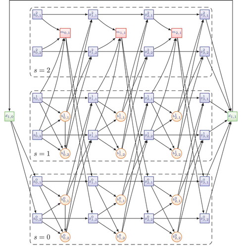
Edges in all the above sets represent different deadheading activities of the vehicles, with the exception of sets $E^{ds},E^{de},E^g,E^f$.

An illustration of the network can be seen in Figure 2. The figure presents a 3-day planning horizon with a single depot, 2 garages, 2 daily vehicle blocks, and 1 maintenance location. The two blocks on the first day are block-compatible (given by edges $(b_{0,1}^0,b_{0,2}^0)$ and $(b_{0,1}^1,b_{0,2}^1)$). The parameter $s$ for maximal days in service before inspection is set to 2, which can be seen on the three state layers of the network ($s=0,1,2$, represented by the dashed rectangles in the figure).

Figure 2. Illustration of the underlying model.

Using the node set $N=\left\{B\cup D\cup G\cup M\right\}$ and edge set $E=\left\{E^{ds}\cup E^{de}\cup E^{bs}\cup E^{be}\cup E^{bc}\cup E^{is}\cup E^{ie}\cup E^g\cup E{}^f\right\}$ the multi-commodity network $(N,E)$ can be defined. This network will have $d$ separate commodities, one for every depot. The commodities of this network will be denoted by $c\in D$. For each edge $e$ of this network, we give an integer vector $x_e$. This vector will have one component for every commodity $c$, which will be denoted by $x_e^c$. The value $x_e^c$ represents if a vehicle from depot $c$ can be assigned the traveling activity connected to edge $e$ (servicing a block, undertaking maintenance, heading to a garage, staying at a garage). Edges $E^{ds}$, $E^{de}$, $E^f$ are added for the respective commodity of the depot they represent, while edges in $E^{bs}$ and $E^{be}$ are created for every depot $d$ that is able to execute the corresponding block. Other edges are available for all commodities. Notations ${\delta }^{+}(n)$ and ${\delta }^{-}(n)$ are used to denote the set of arcs leaving node $n$ and entering node $n$, respectively. Based on the above data, a mathematical model can be given for the problem, and the list of the most important notations regarding this can be seen in the Appendix. The model is formalized the following way:

$\mathrm{m}\mathrm{i}\mathrm{n}\sum _{c\in D}\sum _{e\in E}t{r}_e^c{x}_e^c$

s.t.

(1) $\sum _{c\in D}\sum _{e\in {\delta }^{-}({\mathcal{B}}_{i,j})}{x}_e^c=1,\{\mathrm{\forall }(i,j):1\le i\le n,1\le j\le S(dt(i))\}$(1)

(2) $\sum _{e\in {\delta }^{+}(d_{c,0})}{x}_e^c\le kd(c),\mathrm{\forall }c\in D$(2)

(3) $\sum _{c\in D}\sum _{e\in {\delta }^{-}({\mathcal{G}}_{i,j})}{x}_e^c\le kg(j),\{\mathrm{\forall }(i,j):1\le i\le n,1\le j\le l\}$(3)

(4) $\sum _{c\in D}\sum _{e:(i,m)\in E^{is}}{x}_e^c\le km(j),\mathrm{\forall }m\in M$(4)

(5) $\sum _{e\in {\delta }^{-}(n)}{x}_e^c-\sum _{e\in {\delta }^{+}(n)}{x}_e^c=0,\mathrm{\forall }n\in N,c\in D$(5)

(6) $x_e^c\in \left\{0,1\right\},\mathrm{\forall }e\in \left\{E^{ds}\cup E^{de}\cup E^{bs}\cup E^{be}\cup E^{bc}\right\}$(6)

(7) $x_e^c\ge 0\mathrm{i}\mathrm{n}\mathrm{t}\mathrm{e}\mathrm{g}\mathrm{e}\mathrm{r},\mathrm{\forall }e\in \left\{E^g\cup E^{is}\cup E^{ie}\cup E{}^f\right\}$(7)

Constraint (1) determines that a block has to be serviced by exactly one vehicle. Constraint (2) gives the vehicle limits for every depot at the beginning of planning period, while (3) defines capacities for every garage at the end of every day. Constraint (4) sets the daily limits of the maintenance nodes, the possible incoming vehicles for a maintenance node $m\in M$ on day $i$ being represented by edges $E_{i,m}^{is}\subseteq E^{is}$. Flow conservation for every node of the network is given by (5), while constraints (6) and (7) provide the binary and integrality constraints for all the variables.

The objective of the model is to minimize the arising vehicle and travel costs: the cost of a vehicle from commodity $c$ to service the travel activity denoted by edge $e$ is given by $t{r}_e^c$, the travel cost of a vehicle from depot $c$ to cover the distance denoted by edge $e$. If the edge is a travel activity during which the vehicle leaves its current garage, then the cost of the edge is given by $t{r}_e^c+d{c}^c$ instead, there $d{c}^c$ is the one-time daily cost of a vehicle from depot $c$.

Test results

The model was tested both on real-life and randomly generated input. Important characteristics of both input types, and the solution processes are presented in this section, and the achieved results are also analyzed.

The mathematical model was solved using the Gurobi MIP solver, and ran on a PC with and Intel Core i7 3.30 GHz processor using 32 GB RAM. The time limit for the solver was set to 1 day (86 400 s), and the solver optimality gap tolerance was set to 0.00%. This way, the solution process could terminate only on two conditions: either by finding the optimal solution, or by reaching the designated time limit.

Real-life instances

The real input was part of a ‘what-if’ scenario, trying to coordinate the transportation of three regions in Hungary. The companies in these regions organized their transportation semi-independently before. The transportation companies provided input for a 3-week long planning period, which consisted of vehicle blocks belonging to 7 different day-types. The important features of the input data can be seen in Table 1.

Table 1. Real input characteristics.

Vehicles	238
Garages	109
Maintenance locations	6
Average daily blocks	131

Vehicles of the input were separated into three different depots. Vehicles belonging to depot 3 were able to execute any of the vehicle blocks, while vehicles in depot 1 could execute blocks belonging to either depot 1 or 2. Vehicle of depot 1 could not execute blocks belonging to other depots. Blocks of the daily schedules were not block-compatible, meaning that a vehicle could only service a single block on any given day. Using the input data above, we created two main groups of test instances: one with all three vehicle types, and another with depots 2 and 3 merged into a single type. We ran tests for the entire planning period of 3 weeks and smaller intervals of 1 and 2 weeks also. Values between 2 and 6 were all used as the parameter $s$ of maximum working days for every instance type. Different combinations of the above parameters result in a total number of 30 different instances for the real-life input. The model was solved using the constraints introduced at the beginning of the section.

The results of the mathematical model on the above real-life instances can be seen in Table 2. Each row of the table presents solution data for a single independent test run; it gives the number of depots used for the problem, the length of the planning period (in weeks), and the value of parameter $s$ (the number of maximum days that a vehicle can spend in service before going to maintenance). It also gives the size (rows and columns) of the resulting mathematical model (denoting the number of constraints and variables), and shows the solution time of the problem (in seconds), with the optimality gap of the achieved result.

Table 2. Results for the real-life instances.

Depots	Weeks	s	Columns	Rows	Time (s)	Gap (%)
2	1	2	397 694	8 422	1 038	0.00
		3	591 051	11 026	114	0.00
		4	784 408	13 630	86	0.00
		5	977 765	16 234	84	0.00
		6	1 171 122	18 838	114	0.00
	2	2	799 652	16 232	5 520	0.00
		3	1 188 717	21 234	4 663	0.00
		4	1 577 782	26 236	2 207	0.00
		5	1 966 847	31 238	15 358	0.05
		6	2 355 912	36 240	29 345	0.00
	3	2	1 201 610	24 042	67 195	0.00
		3	1 786 383	31 442	48 705	0.00
		4	2 371 156	38 842	51 261	0.04
		5	2 955 929	46 242	77 546	0.05
		6	3 540 702	53 642	56 165	0.03
3	1	2	544 730	11 702	585	0.00
		3	808 860	15 487	128	0.00
		4	1 072 990	19 272	40	0.00
		5	1 337 120	23 057	39	0.00
		6	1 601 250	26 842	57	0.00
	2	2	1 094 569	22 467	3 395	0.00
		3	1 625 712	29 725	19 431	0.00
		4	2 156 855	36 983	25 304	0.04
		5	2 687 998	44 241	6 840	0.00
		6	3 219 141	51 499	21 640	0.00
	3	2	1 644 408	33 232	16 323	0.01
		3	2 442 564	43 963	22 957	0.04
		4	3 240 720	54 694	81 941	0.23
		5	4 038 876	65 425	79 146	0.37
		6	4 837 032	76 156	52 454	0.78

It can be seen from the table that solutions of a 1-week period are easily reachable, and in most cases, optimal results can also be acquired for a longer planning period of 2 weeks. Almost optimal solutions are also obtainable for the large instances of the 3-week-long period. This is especially important when considering the practical application of the model, as the results are promising regarding both the runtimes and the qualities of the solutions. The easy modification of the parameter $s$ can also help in testing different scenarios for making future decisions.

Random instances

Our random input data was generated in two steps. First, random VSP inputs were created using the method in Dávid and Krész (2013). These instances had 100, 500, or 1000 trips, and used either 2 or 3 depots. A total of 60 instances were generated this way, 10 for every depot-trip combination. Solving the VSP for all these instances resulted in daily vehicle schedules, which were then used as an input for the schedule assignment problem.

Each vehicle schedule was used as the input of a planning period with a single day-type, and planning periods of 1, 2, and 3 weeks were all considered for every schedule. Values between 2 and 6 were all used as the parameter $s$ of maximum working days for every instance type. Considering all combinations of the above parameters, we achieved optimal solutions for a total of 900 test runs. Important features of these input instances are given by Table 3.

Table 3. Random input characteristics.

Trips	Average vehicles	Garages	Maintenance locations	Average daily blocks
100	51	30	2	17
500	219	40	3	55
1000	433	60	4	99

The aggregated results of the instances presented above can be seen in Table 4. Each row of the table provides optimal results for three different instance sets, every set representing one of three problem sizes (100, 500, or 1000 trips). The problem size of a set is given by its column header, while additional parameters of these sets are presented in the header of the row: the number of depots, length of the planning period (in weeks), and the value of parameter $s$ for maximum working days. Each set presents the aggregated results of 10 different test instances, giving average model size and running time of the optimal solutions.

Table 4. Aggregated results for 900 random test runs.

			100 trips			500 trips			1000 trips
Depots	Weeks	s	Columns	Rows	Time (s)	Columns	Rows	Time (s)	Columns	Rows	Time (s)
2	1	2	15 787	1 135	0.79	67 641	2 423	2.37	177 985	4 044	7.35
		3	23 335	1 475	1.73	101 001	3 104	4.48	266 077	5 169	8.88
		4	30 883	1 814	1.35	134 361	3 785	3.99	354 169	6 293	8.98
		5	38 431	2 153	1.52	167 721	4 466	3.98	442 261	7 418	8.99
		6	45 979	2 493	2.04	201 081	5 148	3.12	530 353	8 543	10.28
	2	2	31 453	2 177	4.22	135 121	4 722	11.50	355 729	7 904	27.50
		3	46 519	2 826	7.84	201 801	6 044	42.04	531 853	10 093	329.77
		4	61 585	3 474	15.51	268 481	7 366	144.63	707 977	12 282	462.19
		5	76 651	4 123	39.01	335 161	8 689	268.54	884 101	14 472	683.01
		6	91 717	4 772	92.19	401 841	10 011	206.11	1 060 225	16 661	372.70
	3	2	47 119	3 219	7.48	202 601	7 020	31.31	533 473	11 763	127.11
		3	69 703	4 177	47.62	304 281	9 026	297.94	797 629	15 018	816.75
		4	92 287	5 153	225.45	402 601	10 948	10 115.95	1 059 321	18 273	25 449.56
		5	114 871	6 093	6 626.98	502 601	12 911	4 752.78	1 333 186	21 621	30 154.33
		6	137 455	7 051	6 682.53	602 601	14 875	6 374.63	1 598 791	24 889	51 144.84
3	1	2	23 431	1 208	0.76	90 713	2 521	2.97	235 609	4 259	10.51
		3	34 801	1 566	3.00	135 609	3 227	6.41	352 513	5 438	27.78
		4	46 171	1 923	2.94	180 505	3 932	9.76	469 417	6 617	32.84
		5	57 541	2 281	2.70	225 401	4 638	10.92	586 321	7 795	40.54
		6	68 911	2 638	3.48	270 297	5 344	6.01	703 225	8 974	13.11
	2	2	46 741	2 323	3.62	181 265	4 918	11.48	470 977	8 335	52.82
		3	69 451	3 008	18.60	271 017	6 289	51.55	704 725	10 632	527.44
		4	92 161	3 693	34.05	360 769	7 660	363.30	938 473	12 929	2 091.90
		5	114 871	4 378	61.79	450 521	9 032	533.76	1 172 221	15 226	2 843.32
		6	137 581	5 063	116.72	540 273	10 403	1 015.38	1 405 969	17 524	2 015.59
	3	2	70 051	3 437	5.88	271 817	7 314	39.74	706 345	12 410	125.09
		3	104 101	4 450	50.30	406 425	9 352	499.80	1 056 937	15 826	1 644.36
		4	138 151	5 463	619.36	541 033	11 389	2 531.34	1 402 041	19 197	41 684.79
		5	172 201	6 476	9 622.47	675 641	13 426	7 038.57	1 751 261	22 605	51 468.83
		6	206 251	7 488	3 401.35	810 249	15 463	25 688.33	2 100 481	26 014	97 058.60^a

aThe running time limit was relaxed for four test runs of this instance set in order to achieve optimal solutions in all 900 test cases. See Subsection 5.2 for details.

Our preliminary test runs for the 900 instances in Table 4 were all executed with the same constraints as mentioned before at the beginning of Section 5. We managed to solve 896 instances to optimality this way within the given time. The remaining four instances all belonged to the set of three depot problems for a 3-week planning period with the parameter $s=6$ for maximum working days. The optimality gaps for their results we achieved within the time limit were 0.02, 0.03, 0.003, 0.02%, respectively. As these solutions are near-optimal and we received optimal results for all other test runs, we decided to solve these four instances also to optimality without the limit on running time; thus, not needing to include data for optimality gaps in the table. Because of this, the table presents an average running time that is greater than the 1-day limit for the last instance set. The above results are also promising, as solutions can easily be obtained for random input of different sizes and parameter combinations. The size of the largest problem sets presented in the table (with the average of 99 daily blocks) can be equivalent to the networks of some regions; thus, the given model and solutions process can also be applied to real-life instances with similar characteristics.

As it can be seen both from the real-life and randomized test results, there are three main factors influencing problem size and running time. One of these is the value of the parameter $s$. As the state of the vehicles has to be tracked throughout the network, a separate layer is created for each such state. This basically means the duplication of all garage and block nodes, and these result in more constraints and variables to the problem (capacity constraints and flow conservation) as well as more variables.

Using a heterogeneous fleet with multiple depots also results in an increased number of constraints. Each depot has its own commodity in the network, and similarly to state layers, both flow conservation and node capacities have to be checked separately for every depot. Moreover, there are also constraints linking these different commodities; constraints ensuring that each block is serviced exactly once

Naturally, the length of the planning period also influences the size of the model. As the schedules of a single week are usually more or less similar in structure, the number of decision variables and constraints is expected to grow in a somewhat linear proportion to the number of weeks considered by the problem. This effect can be observed on the sizes of both the real-life and the randomly generated problems.

The combination of the above three factors (parameter $s$, number of depots and size of the planning period) contribute together to the problem size and solution running time. It can be seen from both the real-life and random test results that instances with a 1-week planning period are easily solvable in a short time regardless of number of blocks, depots, or $s$. This is also true in the case of most test instances with a 2-week planning period, slower running times only occurred for some problems with a higher (four or greater) value of $s$. The only instance types that constantly resulted in slow running times are the ones with a 3-week planning period, and a value $s\ge 4$. Yet, even solutions for these instances achieved within the given time limit of 1-day were optimal or near-optimal.

Several types of optimization problems exist for public bus transportation, and the most important characteristics of their results vary depending on the area of their application. For instance, the vehicle rescheduling problem, which addresses unforeseen events occurring during the execution of a pre-planned schedule, has to be solved almost instantly, as the solutions are needed as soon as possible to restore the order of transportation. Here, the running time is more important than the quality of the results. On the other hand, solving the VSP for a single day should yield better quality solutions, while also not taking exceptionally long, especially when the results are only used as suggestions in a decision support system, where experts of the company want to experiment with several different parameter configurations for the same problem. In both of these cases, however, optimality is only a secondary requirement, as the results are only used by the experts of a company as suggestions in their decision-making process.

As opposed to the above problem types, the long running times for the larger instances of schedule assignment are still acceptable when considering its practical application. As these instances have to be solved only once to produce results for a several-week-long horizon, companies can afford even multiple hours of running time when solving such complex problems over a longer planning period. If these solutions are near optimal, and they can be applied in practice, then even the maximum running time of one day that we set for the solver is acceptable for a single execution.

The model yielded good solutions for real-life data that connected the transportation of three different regions, and gave results for a significant planning period of 3 weeks. The largest random instance sets are also comparable with similarly sized real-life scenarios, meaning that the model can be applied generally to such problems.

Conclusions

This article introduces the schedule assignment problem for intercity bus transportation over a planning period, where the daily vehicle blocks are assigned to buses of a transportation company. Important requirements like daily parking and preventive maintenance have to be taken into account due to the long-term nature of the task. To our knowledge, this exact resulting problem has not been considered before in the literature of bus transportation.

We present a mathematical model for the problem using a state-expanded multi-commodity network, which is then solved with the Gurobi MIP solver. Both real-life and random instances are used as an input, and the results are promising for different number of vehicle types and varying parameters for the time limit of the preventive maintenance.

Parking and maintenance constraints considered for the model are only basic requirements of such an assignment, and the model can be further extended to incorporate more sophisticated needs. One such example is the consideration ‘vehicle history’ (different beginning states) at the beginning of the planning period, which could easily be achieved by modifying the definition of vehicle node in the model.

Disclosure statement

No potential conflict of interest was reported by the authors.

Additional information

Funding

The authors acknowledge the support of the Dél-alföldi Közlekedésfejlesztési Klaszter, and the National Research, Development and Innovation Office NKFIH Fund No. [SNN-117879]. Miklós Krész also acknowledges the European Commission for funding the InnoRenew CoE project [Grant Agreement #739574] under the Horizon2020 Widespread-Teaming program and the support of the EU-funded Hungarian grant [EFOP-3.6.2-16-2017-00015].

Appendix:

List of Notations Used in the Mathematical Model

Table

$B$	Set of vehicle blocks
$D$	Set of depots
$G$	Set of garages
$M$	Set of maintenance locations
$N$	Set of all nodes
$E^{bs}$	Set of block starting edges
$E^{be}$	Set of block ending edges
$E^g$	Set of garage waiting edges
$E^{is}$	Set of inspection starting edges
$d_{i,0}$	The node representing vehicles of depot $i$ at the beginning of the planning period
$kd(i)$	Capacity of depot $i$
$kg(i)$	Capacity of garage $i$
$km(i)$	Capacity of maintenance location $i$

References

- Árgilán, V., J. Balogh, J. Békési, B. Dávid, G. Galambos, M. Krész, and A. Tóth. 2014. “ Ütemezési feladatok az autóbuszos közösségi közlekedés operatív tervezésében: Egy áttekintés”, Alkalmazott Matematikai Lapok 31: 1-40. ISSN 0133–3399
- Bertossi, A. A., P. Carraresi, and G. Gallo. 1987. “On Some Matching Problems Arising in Vehicle Scheduling Models.” Networks 17 (1): 271–281. doi:10.1002/net.3230170303.
- Bodin, L., and B. Golden. 1981. “Classification in Vehicle Routing and Scheduling.” Networks 11 (1): 97–108. doi:10.1002/net.3230110204.
- Bodin, L., B. Golden, A. Assad, and M. Ball. 1983. “Routing and Scheduling of Vehicles and Crews: The State of the Art.” Computers and Operations Research 10 (1): 63–212. doi:10.1016/0305-0548(83)90030-8.
- Borndörfer, R., M. Reuther, T. Schlechte, K. Waas, and S. Weider. 2015. “Integrated Optimization of Rolling Stock Rotations for Intercity Railways.” Transportation Science 50 (3): 863–877. doi:10.1287/trsc.2015.0633.
- Borndörfer, R., M. Reuther, T. Schlechte, and S. Weider. 2011. “A Hypergraph Model for Railway Vehicle Rotation Planning.” In 11th Workshop on Algorithmic Approaches for Transportation Modelling, Optimization and Systems, Schloss Dagstuhl–Leibniz-Zentrum fuer Informatik, edited by Alberto Caprara and Spyros Kontogiannis, September 8, 146–155.Saarbrücken/Wadern, Germany: Schloss Dagstuhl – Leibniz-Zentrum für Informatik GmbH, Dagstuhl Publishing.
- Borndörfer, R., M. Reuther, T. Schlechte, and S. Weider. 2012. “Vehicle Rotation Planning for Intercity Railways.” In Proceedings Conference on Advanced Systems for Public Transport, 11–12.
- Bunte, S., and N. Kliewer. 2009. “An Overview on Vehicle Scheduling Models.” Journal of Public Transport 1 (4): 299–317. doi:10.1007/s12469-010-0018-5.
- Ceder, A. A. 2011. “Optimal Multi-Vehicle Type Transit Timetabling and Vehicle Scheduling.” Procedia-Social and Behavioral Sciences 20: 19–30. doi:10.1016/j.sbspro.2011.08.005.
- Dávid, B. 2016. “Schedule Assignment for Vehicles in Inter-City Bus Transportation over a Planning Period.” In Middle-European Conference on Applied Theoretical Computer Science (MATCOS 2016): Proceedings of the 19th International Multiconference INFORMATION SOCIETY - IS 2016, 9–12.
- Dávid, B., and M. Krész. 2013. “Application Oriented Variable Fixing Methods for the Multiple Depot Vehicle Scheduling Problem.” Acta Cybernetica 21 (1): 53–73. doi:10.14232/actacyb.21.1.2013.5.
- Dávid, B., and M. Krész. 2017. “The Dynamic Vehicle Rescheduling Problem.” Central European Journal of Operations Research 25 (4): 809–830. doi:10.1007/s10100-017-0478-7.
- de Matta, R., and E. Peters. 2009. “Developing Work Schedules for an Inter-City Transit System with Multiple Driver Types and Fleet Types.” European Journal of Operational Research 192 (3): 852–865. doi:10.1016/j.ejor.2007.09.045.
- Ernst, A. T., H. Jiang, M. Krishnamoorthy, and D. Sier. 2004. “Staff Scheduling and Rostering: A Review of Applications, Methods and Models.” European Journal of Operational Research 153 (1): 3–27. doi:10.1016/S0377-2217(03)00095-X.
- Giacco, G. L., A. D’Ariano, and D. Pacciarelli. 2014. “Rolling Stock Rostering Optimization under Maintenance Constraints.” Journal of Intelligent Transportation Systems 18 (1): 95–105. doi:10.1080/15472450.2013.801712.
- Giacco, G. L., D. Carillo, A. D’Ariano, D. Pacciarelli, and Á. G. Marn. 2014. “Short-Term Rail Rolling Stock Rostering and Maintenance Scheduling.” Transportation Research Procedia 3: 651–659. doi:10.1016/j.trpro.2014.10.044.
- Guedes, P. C., and D. Borenstein. 2015. “Column Generation Based Heuristic Framework for the Multiple-Depot Vehicle Type Scheduling Problem.” Computers & Industrial Engineering 90: 361–370. doi:10.1016/j.cie.2015.10.004.
- Haghani, A., and Y. Shafahi. 2002. “Bus Maintenance Systems and Maintenance Scheduling: Model Formulations and Solutions.” Transportation Research Part A: Policy and Practice 36 (5): 453–482.
- Lai, Y.-C., D.-C. Fan, and K.-L. Huang. 2015. “Optimizing Rolling Stock Assignment and Maintenance Plan for Passenger Railway Operations.” Computers & Industrial Engineering 85: 284–295. doi:10.1016/j.cie.2015.03.016.
- Laurent, B., and J.-K. Hao. 2009. “Iterated Local Search for the Multiple Depot Vehicle Scheduling Problem.” Computers & Industrial Engineering 57 (1): 277–286. doi:10.1016/j.cie.2008.11.028.
- Mesquita, M., M. Moz, A. Paias, J. Paixão, M. Pato, and R. Ana. 2011. “A New Model for the Integrated Vehicle-Crew-Rostering Problem And A Computational Study on Rosters.” Journal of Scheduling 14 (4): 319–334. doi:10.1007/s10951-010-0195-8.
- Ojo, T. K. 2017. “Quality of Public Transport Service: An Integrative Review and Research Agenda.” In Transportation Letters, 1–14. Taylor & Francis doi:doi.10.1080/19427867.2017.1283835
- Orloff, C. S. 1976. “Route Constrained Fleet Scheduling.” Transportation Science 10 (2): 149–168. doi:10.1287/trsc.10.2.149.
- Peters, E., R. de Matta, and W. Boe. 2007. “Short-Term Work Scheduling with Job Assignment Flexibility for a Multi-Fleet Transport System.” European Journal of Operational Research 180 (1): 82–98. doi:10.1016/j.ejor.2006.02.032.
- Saha, J. L. 1970. “An Algorithm for Bus Scheduling Problems.” Journal of the Operational Research Society 21 (4): 463–474. doi:10.1057/jors.1970.95.
- Zeynep, F. Z., C. Altunta, and D. C. Tulazoğlu. 2017. “Multi-Objective Integrated Acyclic Crew Rostering and Vehicle Assignment Problem in Public Bus Transportation.” OR Spectrum 39 (4): 1071–1096. doi:10.1007/s00291-017-0485-z.