The impact of autonomous vehicles on urban traffic network capacity: an experimental analysis by microscopic traffic simulation

ABSTRACT

Urban commuters have been suffering from traffic congestion for a long time. In order to avoid or mitigate the congestion effect, it is significant to know how the introduction of autonomous vehicles (AVs) influence the road capacity . The effects that AVs bring to the macroscopic fundamental diagram (MFD) were investigated through microscopic traffic simulations. This is a key issue as the MFD is a basic model to describe road capacity in practical traffic engineering. Accordingly, the paper investigates how the different percentage of AVs affects the urban MFD. A detailed simulation study was carried out by using SUMO both with an artificial grid road network and a real-world network in Budapest. On the one hand, simulations clearly show the capacity improvement along with AVs penetration growth. On the other hand, the paper introduces an efficient modeling for MFDs with different AVs rates by using the generalized additive model (GAM).

KEYWORDS:

• Autonomous vehicles
• macroscopic fundamental diagram
• urban road
• capacity
• SUMO
• generalized additive model

Introduction

Traffic congestion is now a part of our daily life with examples aplenty. It keeps increasing in metropolitan areas, contributing to great economic losses and causing delay, compromised levels of service, and discomfort during traveling. Congestion may occur when demand for traveling exceeds supply or transport system capacity. The solution to traffic congestion is to balance the demand side and supply side. The rise of supply should match the gain in demand (Triantis et al. 2011). However, it is extremely costly and environmentally damaging to enlarge traffic network capacities by constructing more roads and infrastructure.

There are numerous factors that can influence the road capacity, such as incidents (Lu and Elefteriadou 2013), road geometry (Heaslip, Jain, and Elefteriadou 2011), weather condition and so forth. Besides the road construction and factors mentioned above, the road capacity can also be enlarged by better utilization of the existing infrastructures. In our days and soon, autonomous vehicles change our conventional transportation frameworks. Telematics-based, shared, request responsive mobility services with advanced information administration methods are expected (Szigeti, Csiszár, and Dávid 2017). It can possibly fundamentally change the driver interactions and give huge chances to radically boost traffic capacity, efficiency, stability, and safety of existing mobility systems. Accordingly, the paper investigates the impacts of AVs, with a special spotlight on the efficiency of utilizing the existing infrastructure, namely, the capacity of the road network.

Autonomous vehicles are vehicles that are capable of sensing their environment and navigating with less or without human input (Gehrig and Stein 1999). The autonomous driving is grouped into six different levels by the international Society of Automotive Engineers (SAE) according to the amount of driver intervention and attentiveness required. It delivers a harmonized classification system for Automated Driving Systems, specifically SAE J3016 Taxonomy and Definitions for Terms Related to On-Road Motor Vehicle Automated Driving Systems; see Table 1 based on the SAE International (2018).

Table 1. The levels of automation defined in (2018, p. 19).

Level 0 – ‘No automation’	‘The full-time performance by the human driver of all aspects of the dynamic driving task, even when enhanced by warning or intervention systems.’
Level 1 – ‘Driver Assistance’	‘The driving mode-specific assistance system of execution by a driver either steering or acceleration/deceleration using information about the driving environment and with the expectation that the human driver performs all remaining aspects of the dynamic driving task.’
Level 2 – ‘Partial Automation’	‘The driving mode-specific execution by one or more driver assistance systems of both steering and acceleration/deceleration using information about the driving environment and with the expectation that the human driver performs all remaining aspects of the dynamic driving task.’
Level 3 – ‘Conditional Automation’	‘The driving mode-specific performance by an automated driving system of all aspects of the dynamic driving task with the expectation that the human drivers respond appropriately to a request to intervene.’
Level 4 – ‘High Automation’	‘The driving mode-specific performance by an automated driving system of all aspects of the dynamic driving task, even if a human driver does not respond appropriately to a request to intervene.’
Level 5 – ‘Full Automation’	‘The full-time performance by an automated driving system of all aspects of the dynamic driving task under all roadway and environmental conditions that can be managed by a human driver.’

Based on the literature review, the introducing AVs to the road network can improve capacity by i) keeping traffic flow parameters steady, and ii) taking into account faster responded, more tightly spaced vehicles. Utilizing simulations, various studies investigated the shifts in microscopic driving behavior in AVs. For example, the reaction time, acceleration, deceleration, platoon size, and their impacts on-road capacity were studied. If AVs were operated at shorter headway, then maximum throughput could generally boost. On the contrary, an increasingly headway would lead to the opposite impact on the road capacity. If vehicles were operated at lower speeds so as to make the vehicle flow more stable, this could cut down the capacity of a bottleneck. At the same time, the delay and travel time would increase (Jerath and Brennan 2012; Kesting et al. 2008; Talebpour and Mahmassani 2016; Talebpour, Mahmassani, and Elfar 2017; Van Arem, Van Driel, and Visser 2006). Van Arem, Van Driel, and Visser (2006) investigated the impacts of vehicle platoon size on the flow stability and capacity on a freeway with a lane drop by using a microscopic simulator, MIXIC. Most of these researches revealed that an intermediate (or even lower) AVs penetration rates could contribute to a considerable capacity upgrading (Jerath and Brennan 2012). With the help of simulation software, Talebpour, Mahmassani, and Elfar (2017) found the throughput was enhanced considerably when the AVs penetration rate exceeded 30% as they studied the influences of assigning a lane of a four-lane freeway to AVs on the traffic flow dynamics and trip time reliability. Van Arem, Van Driel, and Visser (2006) found that significant impacts were noticed only when the AVs penetration exceeded 40%. Likewise, Jones and Philips (2013) found that the positive impact of Cooperative Adaptive Cruise Control (CACC) vehicle on the traffic flow stability and throughput was realized if the CACC vehicle penetration surpassed 40%. In contrast, Van Arem, Van Driel, and Visser (2006) spotted the capacity increment was negligible unless the AVs penetration rate was above 50% in simulation. Shladover (2012) obtained the consistent outcome by utilizing field experiments. While Tientrakool, Ya-Chi, and Maxemchuk (2011) found that capacity improved slightly until the CACC penetration rate exceeded 85%. One hundred percent AVs penetration scenario contributes a more noteworthy positive impact on the road capacity. For instance, Friedrich (2016) found that a capacity increase of 40% could be achieved with purely autonomous vehicles in city traffic, while capacity could be improved on highway sections by about 80%. Olia et al. (2018) found that the purely cooperative vehicle scenario can raise the highway capacity by 300% compared to the traditional vehicles’ scenario. However, in his work, concerning the adoption of AVs in the vehicle fleet, the realizable capacity improvement shows relatively indifferent to the AVs penetration.

In most of the articles mentioned above, connected AVs were considered and these works focused on freeway traffic. Solely Tientrakool, Ya-Chi, and Maxemchuk (2011) have investigated the AVs impacts on urban road capacity, but his work concentrated only on the impacts at a single intersection and not on a whole urban traffic network. Our paper concentrates on the effects of AVs without connected technology by defining the vehicles with different parameters compared to the conventional cars in SUMO simulator. In addition, the simulation analysis was carried out in two typical urban road networks: a virtual grid network and a real-world road system in Budapest. This article aims to investigate the possible impacts of AVs on the urban traffic network capacity.

There exist two basic macroscopic traffic flow modeling approaches in the literature: three-phase traffic flow theory and Macroscopic Fundamental Diagram (MFD), to choose from to analyze the data. In the three-phase traffic flow theory the capacity of road is not a constant value but infinite numbers within a range of the flow rate between a minimum and maximum capacity (Kerner 2016). It would add unnecessary complexity to the estimation of AVs’ impacts on the road capacity. Therefore, MFD was chosen to estimate the capacity of the roads. Capacity of a route is the maximum hourly rate at which persons or vehicles can move in a reasonable order of a point or a lane of road (Manual, Highway Capacity 2000). The maximum flow rate is easily to be found with the help of MFD. The idea of urban MFD has been generally researched in the previous decades, e.g. Mahmassani, Williams, and Herman (1987), Daganzo (2007), Keyvan-Ekbatani, Papageorgiou, and Papamichail (2014), Csikós, Tettamanti, and Varga (2015), He, He, and Guan (2014), Geroliminis and Daganzo (2008). Furthermore, Guan and Shuyan (2008) found that the three-phase traffic theory and fundamental diagram are not conflicting when it comes to the urban area. MFD can be utilized to describe the service level as well as the throughput of a traffic system. When applying inflow regulation or speed limits to the road, the MFD is also valid to define the traffic dynamics. The fundamental diagram is basically given by the graph of flow–density relationship. Besides, MFD is also related with the macroscopic average speed (i.e. space mean speed on a given link or network) in the forms of speed-density and speed-flow functions. These diagrams could be easily derived by plotting field data points and applying appropriate curve fitting method to the scatter plots.

This paper is organized as follows. Section 2 presents the theoretical preliminaries on MFD and the calculation method for the macroscopic variables. Section 3 contains the SUMO simulator’s settings, AVs modeling methodology, and the MFD curve fitting method. Section 4 discusses the core outcomes of the simulation experiment, while concluding remarks are provided in Section 5.

Theoretical foundations

In this part, the macroscopic model of urban road traffic network is discussed. Then, the calculation method of the measured data by SUMO is introduced.

Macroscopic model for urban traffic

In this research, the impacts of AVs penetration on the MFD have been investigated. The work was carried out with SUMO simulations by applying different percentage of both conventional cars and full automation AVs. The simulations were operated in a real-world traffic network and a virtual grid road network considering different penetration rates. The simulator virtually measured the traffic volume on each link and the whole network’s throughput. Data were obtained through a macroscopic link-level measurement that called ‘edgeData’ measurement in SUMO (Krajzewicz et al. 2012). The outcomes were calculated to understand the development of different situations and to make known how the traffic network capacity changes along with different penetration levels of self-driving cars.

The macroscopic fundamental diagram of traffic flow defines the relationship among the traffic flow $Q(vehicles/h$), the vehicle concentration $\rho$ ($vehicles/km$) and the space mean speed $V$ ($km/h$) (Williams et al. 1987). The MFD is based on the fundamental equation:

(1) $Q(\rho )=\rho \cdot V(\rho ).$(1)

As described in the previous section, the fundamental diagram can be applied in both network-level and link-level. The network-level MFD models the throughput of the traffic network per hour:

(2) $Q_N({\rho }_a),$(2)

where $Q_N$ is the number of vehicles that pass through the network. ${\rho }_a$ is the average density of the network, and it simply equals to the known total number of vehicles in the network divided by the sum of all link lengths of the road network, i.e.

(3) ${\rho }_a=\frac{{{\sum }_{i=1}^n{\rho }_{i}l}_i}{{\sum }_{i=1}^n{l}_i},$(3)

where $l_i$ is the length of link $i$, $n$ is the number of links (Williams et al. 1987; Csikós, Tettamanti, and Varga 2015). The second approach interprets the MFD of one single road link of the network, i.e.

(4) $Q_i({\rho }_i)={\rho }_i\cdot V_i({\rho }_i),$(4)

where $Q_i$ is the flow, ${\rho }_i$ means the density, $V_i({\rho }_i)$ defines the mean velocity, and $Q_i$ is the flow on link $i$.

Calculation based on SUMO measurements

All trip histories of the vehicles going through the traffic network were collected to utilize these observations in the MFD parameter estimation later. The edge-based measurement of SUMO gave link-level concentration, stop time, overlap travel time, sample second and average speed.

To draw the MFD, concentration $\rho$, network average velocity $V$ and flow $Q$ are needed. The following formula were used for the calculation of these values.

(5) $\rho =\frac{{\sum }_1^n{N}_{vi}}{{\sum }_1^n{l}_i}(veh/km),$(5)

(6) $V=\frac{{\sum }_1^n{V}_i{N}_{vi}}{{\sum }_1^n{N}_{vi}}(km/h),$(6)

(7) $Q=\sum _1^{n}3.6\cdot V_i{\rho }_i(veh/h),$(7)

where $n$ is the number of the links in the traffic network, $V_i$ and $N_{vi}$ are the average speed and vehicle numbers on the $i^{th}$ link during the measurement interval $T$.

Methodology

Some detailed simulation researches were operated within SUMO to analyze the effect of AVs on the urban road system capacity. To have a better observation, the simulations were carried out in two road networks, namely a virtual grid traffic network and a real-world urban road system. In order to determine the impacts of variations in market penetration of conventional and autonomous vehicles, the simulation scenarios were characterized to represent various combinations of both types of vehicles. The experimental setup that applied in the capacity impact estimation comprised all the market penetration levels. The adoption of autonomous vehicles varied from 0% to 100% by stepping with 20%. The results were handled and analyzed with the generalized additive model (GAM) to find the relationship between average speed $V$ and vehicle density $\rho$. Then, with the help of MFD theory, the flow–density relationship with respect to AVs penetration rate could be identified.

SUMO settings

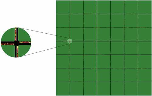
As illustrated in Figure 1, a grid road network was created. It was designed to serve as a common situation of the urban road system, especially in the US. The utilized network was an $8\times 8$ grid, which had 60 nodes and 36 intersections in it. The lengths between adjacent nodes were $300m$. The network links were bidirectional roads with single lanes. As for traffic control, the SUMO built-in tool, which named ‘time gap based’ traffic signal method, was applied. To realize an optimized circulation of traffic light phases dynamically, the controller switches to the next phase when it detects an adequate time opening between successive vehicles (Krajzewicz et al. 2012).

Figure 1. Grid test traffic network.

In the simulations all vehicles get automatically routed at insertion. Routing was created by using trip file of SUMO to form traveling demand, i.e. origin and destination links were defined rather than a whole list of lane links. In this situation, vehicles choose the fastest paths according to the current traffic conditions of the network when they enter. Therefore, the distribution of vehicles is more flexible and homogeneous compared to the demand modeling with fixed routes. The origin and destination links were located in the boundary to keep vehicles running longer.

The demand increased gradually till a traffic congestion formed in the network then decreased to zero smoothly. The simulation scenarios in the paper were generated to obtain significant traffic jams but gridlock was avoided.

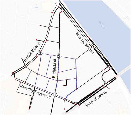
As shown in Figure 2, the real-world study area was located in the ${11}^{th}$ district in Budapest Hungary in the vicinity of Budapest University of Technology and Economics. The network contained five arterial roads: Bartók Béla út, Karinthy Frigyes út, Irinyi József út, Műegyetem rkp., Budafoki út. Simulations were run in the whole road network shown by Figure 2, but the results were evaluated concerning 30 selected road links only (depicted by blue color) forming an intrinsically homogeneous sub-network (based on our local knowledge) for investigation. On the other hand, in order to provide realistic simulation results, it worth simulating a wider context of the specific test area as it is a part of a bigger and complex network. In the SUMO simulation without considering a bigger area, one could not have generated congestion at the perimeter of the network which would have been unrealistic for the chosen real-world test network. The speed limits for all roads were $50km/h$. Link length average was $0.116km$. In these simulations, traditional fixed traffic light signal (TLS) method was applied. Mainly TLS 1, 2, and 3 affected the investigated area (denoted by numbers in Figure 2).

Figure 2. Real-world traffic network (GPS coordinates: 47.47733, 19.05358).

The vehicle flows came from the arterial roads then ran through the investigated area. According to the real-world traffic data, heavy traffic demands were applied to the arterial roads, while small vehicle flows to other side streets. Moreover, for the purpose of MFD estimation, simulations were carried out with varying traffic loads, including the situations from the free flow to the rush hours flow. At the beginning of the simulation, the traffic demand was low. Then, a series of light additional flows were introduced into the network continuously in order to arrive at a congested situation. Finally, demand started decreasing. The amount of vehicles is defined by the departure time in the trip file of SUMO. The Vehicle type distribution was used to define the percentage of AVs.

Modeling autonomous vehicles

The vehicle modeling method is the same with the previous work of Lu and Tettamanti (2018). Default SUMO parameters have been modified in order to model a plausible future for AVs. In the paper the default car following model (Krauss Model) was applied. The parameter selection was related to longitudinal movement, acceleration, deceleration and gap acceptance. These behaviors were formalized as parameters in the car-following model of SUMO. The implemented model followed the idea that let vehicles drive as fast as possible while maintaining perfect safety (always being able to avoid a collision if the leader starts braking within leader and follower maximum acceleration bounds). The following list shows the editable parameters of the Krauss car following model (Krauß 1998):

• Mingap: the offset to the leading vehicle when standing in a jam (in $m$).

• Accel: the acceleration ability of vehicles of this type (in $m/s^2$).

• Decel: the deceleration ability of vehicles of this type (in $m/s^2$).

• Emergency Decel: the maximum deceleration ability of vehicles of this type in case of emergency (in $m/s^2$).

• Sigma: the driver imperfection (between 0 and 1).

• Tau: the driver’s desired (minimum) time headway (reaction time) (in $s$).

For no and full automation vehicles, the deceleration and the emergency deceleration remained the same, considering the safety. The emergency deceleration was set to 8 $m/s^2$. This value was based on the study of Kudarauskas (2007). While the mingap, acceleration and time headway were taken from Atkins Ltd (2016). The parameters are tabulated to Table 2.

Table 2. Parameters of the driver model used in SUMO simulations.

	Mingap ($m$)	Accel ($m/s^2$)	Decel ($m/s^2$)	Emergency decel ($m/s^2$)	Sigma	Time headway ($s$)
No automation	1.5	3.5	4.5	8	0.5	0.9
Full automation	0.5	3.8	4.5	8	0	0.6

Statistical evaluation approach

The output of the simulation experiment introduced earlier in this section is a series of observations at various levels of AVs penetration rates and network-level traffic conditions. Our ultimate goal is to estimate the flow–density relationship of the MFD and observe the way how the share of AVs affects its shape, with a focus of any deviations in the critical density and the corresponding flow level.

To achieve this goal, what we first model and estimate using the simulation outcomes is the speed-density function. This segment of the MFD is closer to a linear relationship, and therefore can be estimated more reliably than the inverse U-shaped flow-density function. We apply a semiparametric approach to model the speed–density relationship. This allows us to relax the assumption that the speed-density function is perfectly linear, i.e. we allow for $\rho$, the traffic density variable, to have a non-parametric impact on average traffic speed, the dependent variable in our regression specification.

We model average speed as

(8) $V(r,\rho )=\alpha +s(\rho )+\beta \cdot r+\gamma \cdot r\rho ,$(8)

where $\alpha$ can be considered as average speed under free-flow conditions, i.e. the intercept of the speed-density function, and $s(\rho )$ is a non-parametric spline estimated together with the prespecified parameters of the model, $\alpha$, $\beta$ and $\gamma$. The ratio of AVs among all vehicles ($r$) enters the regression equation twice. First, it affects the free-flow average speed if the estimate of $\beta$ will become statistically significantly different from zero. Second, it affects the slope of speed-density function through the interaction term between $r$ and $\rho$, provided that the coefficient of this interaction ($\gamma$) will differ from zero after model fitting. That is, $\gamma$ tells whether the presence of AVs induces changes in the way in which increasing traffic density affects average speed. If this parameter is positive and statistically significant, then the negative impact of traffic density on speed will be somewhat weaker with the introduction of AVs. This semiparametric representation can be powerful in prediction because we do not need to make assumptions about the baseline functional form of the speed–density curve a priori.

The estimation of our semiparametric regression specification is applied via a generalized additive model (GAM) implemented in R. GAM is basically a generalized linear model (GLM) in which the predictor depends linearly on covariates that enter the regression with predefined functional form, and unknown smooth functions of other predictor variable(s); in our case a smooth function of traffic density.

For a given level of AVs penetration rate, the more informative flow–density curve, the subject of main interest in the paper, can be recovered with a simple algebraic transformation of the estimated speed-density function. By substituting $V$ in equation (1)(1) $Q(\rho )=\rho \cdot V(\rho ).$(1) into equation (8)(8) $V(r,\rho )=\alpha +s(\rho )+\beta \cdot r+\gamma \cdot r\rho ,$(8) , we get the corresponding flow–density relationship $Q(\rho ;r)$.

In practice, we generate the full sequence of potential density values from zero to the highest density observed in our data, and compute the corresponding speed levels using the estimated model. Then we transform the average speed values into flow, based on the algebraic relationship detailed above. This way we can reproduce the $Q(\rho ;r)$ segment of the MFD for any given AVs ratio $r\in (0,1)$. Identifying the critical density and the corresponding traffic flow level (i.e. the maximum throughput of the network) is a straightforward numerical task, so this approach enables us to express the key parameters of the simulated MFDs in function of the penetration rate of AVs.

Results

With the help of GAM regression model, the simulation data were processed. The results of the grid network and the real-world network are displayed separately in this section. In order to verify the rationality of the GAM, the statistic coefficients were firstly inspected. After the validation of the regression model, the maximum capacity and the corresponding density of different AVs penetration are also investigated.

Results of grid network

The simulation results of grid network are shown in this section. Table 3 shows the summary of speed-AVs ratio–density relationship estimation of grid network simulation results of all scenarios. There were 1760 set of data in the estimation. $R^2$ indicates the goodness of fitting, which is 0.983. So the proposed model is validated for the speed-AVs ratio–density relationship estimation. The $t$-$value$ and $p$-$value$ reflect the significance levels of the independent variables. The $t$-$value$ is a measure of how many standard deviations the estimate coefficient is far away from zero. It is expected to be far away from 0 because this would indicate the null hypothesis is rejected. That is to say, a relationship between velocity and the independent variables mentioned above exists. In this analysis, the $t$-$values$ are relatively far away from 0 and are large relative to the standard error, which could indicate a relationship exists. The $p$-$value$ is the probability when the null hypothesis is true. A small $p$-$value$ for the intercept and independent variables indicates that the null hypothesis is reject. This allows us to conclude that there is a relationship between capacity and the investigated variables. Actually, the $p$-$value$ can be calculated from $t$-$value$. These two values give equivalent conclusions that all investigated terms have a relationship with the response average speed $V$ because the $p$-$values$ of all terms are much less than 0.001.

Table 3. GAM regression of the grid network simulation.

Coefficient	Estimate	Standard error	$t$-$value$	$p$-$value$	$R^2$
$\alpha$	16.237	0.05988	271.129	$<2E-16$	4[2]*0.983
$\beta$	1.298	0.2073	6.264	5.56E-10
$\gamma$	0.024	0.00723	3.372	0.000776
$s(density)$				$<2E-16$

A spline is a piece-wise function defined by polynomials, thus it is not necessary to define its formula in the paper. Instead, the spline regression is shown in Figure 3. The Estimated Degrees of Freedom (EDF) of the smooth term s(density) is 6.603. EDF is the estimated degrees of freedom of the spline. It can be understood as how much given variable is smoothed. Higher EDF value suggests higher complexity of the spline. The dashed lines in the figure are the confidence lines which indicate two standard error bounds. The rug on the horizontal axis is used to visualize the distribution of the data. Figure 4 shows the speed – density relationship of the data from grid network simulation of all scenarios. These data were obtained in six scenarios with a full range of AVs ratios ($0\mathrm{\%},20\mathrm{\%},40\mathrm{\%},60\mathrm{\%},80\mathrm{\%}\mathrm{a}\mathrm{n}\mathrm{d}100\mathrm{\%}$). The AVs ratio was also considered to be a variable in the speed–density relationship estimation. Two lines in Figure 4 represent the regressions of two different AVs penetration. The black line is the speed–density relationship regression of 0% AVs scenario. The blue line is the fitted curve of 100% AVs penetration.

Figure 3. Grid network: spline regression where the EDF value is 6.6 in s(density, EDF).

Figure 4. Grid network data: speed–density relationship.

After obtaining the speed-AVs ratio-density, the flow-AVs ratio-density is easily to get by substituting the speed $V$ in Eq. (1)(1) $Q(\rho )=\rho \cdot V(\rho ).$(1) with the fitted function $V(r,\rho )$ . The fitted flow-AVs ratio-density function is illustrated in Figure 5. The black line is the fitted curve of 0% AVs scenario. The blue line is the regression of purely driverless car scenario data. Based on the fitted flow-AVs ratio–density relationship, the maximum flows and the corresponding densities of different AVs penetration scenarios are marked as black dots, as shown in Figure 5. They are connected to show the change of the capacity and the critical densities with different AVs ratio. From low to high, the ratios of the self-driving cars corresponding to these points are 0%, 10%, 20%,30%,40%, 50%, 60%, 70%, 80%, 90%, and 100%, respectively. The flow-AVs ratio relationship and density-AVs ratio relationship were extracted and plotted in Figures 6 and 7. The relative changes of the scenarios comparison with the zero AVs penetration case are also provided by Table 4. It is observable that the maximum flow is augmenting along with the increase of AVs penetration in an almost linear way. But the final gain of $100\mathrm{\%}$ AVs penetration is only $16.01\mathrm{\%}$, which is less than the theoretically calculated result ($40\mathrm{\%}$) by Friedrich (2016) formerly. This can be explained by the fact that the calculated result by Friedrich (2016) merely took one intersection into consideration which eliminated the accumulation of vehicles on the adjacent roads. The maximum flow has an approximately linear relationship with AVs penetration. The value of the critical density raises slowly in the beginning. Then the increase accelerates after 40% AVs penetration.

Table 4. Grid network data: maximum flow, critical density, and their change !.

AVs penetration rate	0%	10%	20%	30%	40%	50%	60%	70%	80%	90%	100%
Maximum traffic flow (veh/h)	57,016	57,753	58,511	59,293	60,106	60,958	61,865	62,839	63,881	64,983	66,142
Relative change compared to
the zero penetration case	–	1.29	2.62	3.99	5.42	6.91	8.50	10.21	12.04	13.97	16.01
Critical traffic density (veh/km)	23.24	23.7	24.24	24.87	25.68	26.75	28.16	29.7	31.08	32.28	33.38
Relative change compared to
the zero penetration case	–	1.98	4.30	7.01	10.50	15.10	21.17	27.80	33.73	38.90	43.63

Figure 5. Grid network data: estimated flow–density relationship.

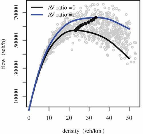
Figure 6. Grid network data: change of the maximum traffic flow according to the AVs penetration ratio.

Figure 7. Grid network data: change of the critical traffic density (the density at the maximum traffic flow) according to the AVs penetration ratio.

Results of real-world network

The calculation and estimation processes were identical with the methods used for the grid road network (presented in previous section). Table 5 shows the speed-AVs ratio–density relationship estimation of the real-world network simulation results in all scenarios. The high value (0.789) of $R^2$ means a high quality of the fitting. In terms of significance test, $t$-$values$ and $p$-$values$ demonstrate all the terms having relationship with the response variable (average speed). The $t$-$values$ are far away from zero and the $p$-$values$ are less than 0.001. This means that the model is also validated for the real-world road network.

Table 5. GAM regression of the real-world network simulation.

Coefficient	Estimate	Standard error	$t$-$value$	$p$-$value$	$R^2$
$\alpha$	21.815	0.1784	122.284	$<2E-16$	4[2]*0.789
$\beta$	1.724	0.51106	3.374	7.57E-04
$\gamma$	0.07	0.02066	3.399	0.000693
$s(density)$				$<2E-16$

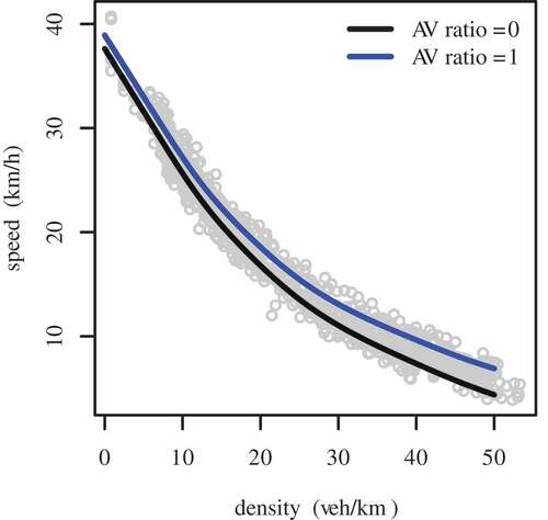
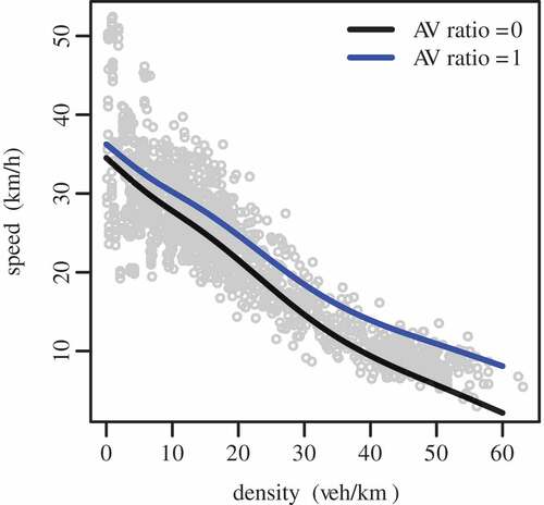
The Estimated Degrees of Freedom (EDF) of the smooth term $s(density)$ is 3.853. The spline regression is illustrated in Figure 8. The confidence lines are depicted as dashed lines in the figure, indicating two standard error bounds. The visualization of the data distribution is illustrated as a rug on the horizontal axis. The estimated speed–density relationship can be found in Figure 9. The gray circles are the simulation data of real-world network in all scenarios. The curves are monotonically decreasing with a concave shape rather than a linear one. The black curve is the regression of all conventional vehicle scenario. The blue line is the fitted speed–density relationship of the purely driverless vehicle scenario.

Figure 8. Real-world network: spline regression where the EDF value is 3.85 in s(density, EDF).

Figure 9. Real-world network data: speed–density relationship.

Figure 10 shows the fitted flow-AVs ratio–density relationship. The gray circles are the simulation data of real-world network in all scenarios. The black curve is fitted with 0% AVs ratio scenario data. The blue line shows the fitted flow–density relationship of purely AVs penetration scenario. In the 100% AVs penetration scenario, a plateau occurs when the flow is around the maximum value. This shows a beneficial property of having AVs in a network. In a range, the density of vehicles can increase without hyper congestion. The maximum traffic flow and the corresponding densities of different AVs penetration scenarios are marked as black dots in Figure 10. These points represent the capacity and critical densities of a range of self-driving cars penetrations which are 0%, 10%, 20%,30%,40%, 50%, 60%, 70%, 80%, 90%, and 100%, respectively, from the bottom to the roof. A line through these dots shows the change of the capacity and the critical densities of different AVs penetration scenarios in the real-world network simulation. Both the maximum flow and the corresponding critical density have an increasing trend with higher AVs penetration. From Figure 11, one can see that the maximum flow, and AVs ratio also have a quasi-linear relationship in the real-world network simulations. The maximum flow boosts with the raise of AVs penetration. Figure 12 shows the traffic concentration changes with the different AVs market penetration scenarios. The critical density is increasing with a higher driverless car penetration. Table 6 shows the maximum flow, the corresponding critical traffic concentration, and their relative comparison with the purely traditional regular vehicle scenario of different AVs penetration scenarios. It shows that a capacity increment value of $23.81\mathrm{\%}$ is achieved with purely autonomous traffic, which is a bit higher than that of the grid network simulations. This may stem from the fact that the real-world network is smaller. The smaller the network is, the less the accumulation of vehicles is. This fact may also lead to higher critical concentration of same AVs penetration than that of the grid network. It also reflects that the increase of the critical traffic density is moderate at the beginning. After 50% of AVs ratio, however, it becomes steep. The benefits of driverless car are more and more obvious with an increasing penetration. In all, the critical traffic concentration has a $48.45\mathrm{\%}$ raise with 100% autonomous vehicle on road.

Table 6. Real-world network data: maximum flow, critical density, and their change !.

AVs penetration rate	0%	10%	20%	30%	40%	50%	60%	70%	80%	90%	100%
Maximum flow (veh/h)	13,497	13,765	14,040	14,324	14,616	14,919	15,234	15,563	15,910	16,283	16,710
Relative change compared to
the zero penetration case (%)	–	1.99	4.02	6.13	8.29	10.54	12.87	15.31	17.88	20.64	23.81
Critical density (veh/km)	25.22	25.67	26.15	26.68	27.25	27.9	28.65	29.57	30.75	32.54	37.44
Relative change compared to
the zero penetration case (%)	–	1.78	3.69	5.79	8.05	10.63	13.60	17.25	21.93	29.02	48.45

Figure 10. Real-world network data: estimated flow–density relationship.

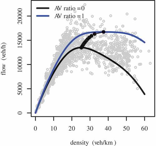
Figure 11. Real-world network data: change of the maximum traffic flow according to the AVs penetration ratio.

Figure 12. Real-world network data: change of the critical traffic density according to the AVs penetration ratio.

Conclusion

This paper investigated the impact of AVs on urban road network capacity. Expectedly, AVs have significant potential to improve traffic capacity, efficiency, stability, and safety of existing mobility systems. The scientific literature has already investigated the potential impacts of AVs use on the transportation system indicating that AVs can improve highway capacity especially when the penetration is high. However, most of the research works focus on highway capacity improvement and just a few studies have addressed the impacts on urban transportation with different AVs adoption. To close this gap, two urban road networks were created to represent typical urban environments: one with grid shape (common in the USA for instance), and another presenting a typical European network (quite irregular considering the street sizes). The traffic demands increased slowly and smoothly to run the simulation over the entire range of demand conditions. The AVs were simulated in the SUMO traffic simulation suite with different driving parameters compared to the conventional vehicles according to the default car following model (Krauss Model). Six scenarios with different AVs penetrations (from 0% to 100%) were simulated for both networks.

In the paper, The GAM regression method was applied to fit the speed-AVs ratio–density relationship firstly. The $R^2$ and $p$-$values$ of the estimation show that the GAM is a validated model for estimating the speed-AVs ratio–density relationship. This implies that it is a reasonable method to estimate MFD as well. The MFDs were constructed based on the fitted relationship. The maximum flow and critical density for all scenarios could be then determined.

The results show that the capacity is increasing quasi-linearly with higher AVs penetration for both grid networks and real-world network. In the grid network, the maximum flow increases by 16.01% considering the 100% AVs penetration scenario with only conventional vehicles. This improvement is less than the theoretically calculated result (40%) of Friedrich (2016). In his work, only a single intersection was taken into consideration which eliminated the accumulation of vehicles on the adjacent roads. That could explain the less increment of this paper because the simulations were carried out in road networks. But, Olia et al. (2018) found much less benefits (8% improvement) from autonomous vehicle. His finding could be attributed to the similar headway settings for autonomous vehicles and regular vehicles. The critical density also increases along with higher AVs penetration. It increases slowly in the beginning. When AVs adoption arrives at 40%, the critical density increases more intensively. For the real-world network simulation, the total increase of maximum flow is around 25% from the 0% AVs penetration to purely AVs scenario. The critical density changes in a similar way with that of the grid network. The critical density increase becomes more intensive around 50% AVs penetration. Moreover, there is an obvious plateau around the max flow in case of 100% AVs on the road.

On the whole, important conclusions can be drawn from the analysis of AVs penetration introduced in the paper. The AVs penetration has a positive impact on improving the road network capacity in a quasi-linear way. Maximum traffic flows in case of 100% AVs penetration are 16-23% larger than that of all conventional vehicle scenario. This improvement is due to shorter headway and less reaction time of autonomous vehicle. Also, the density can augment with higher self-driving vehicle adoption. It increases slowly in the beginning and then intensively around 40% AVs penetration. This means the benefit is not obvious when there is not enough driverless cars on the road as the autonomous vehicles must adapt itself to the conventional vehicles obviously. When self-driving cars start dominating the roads, a plateau occurs around the maximum flow. This phenomenon means that no significant maximum is obtained, i.e. maximum throughput is available on a longer area and not at a dedicated point (critical density of conventional MFDs). With the adoption of 100% autonomous vehicle, the road network becomes more stable and can avoid getting congested easily to some extent.

Correction Statement

This article has been republished with minor changes. These changes do not impact the academic content of the article.

Acknowledgments

The research work was supported by the Hungarian Government and co-financed by the European Social Fund (EFOP-3.6.3-VEKOP-16-2017-00001: Talent Management in Autonomous Vehicle Control Technologies) and by the János Bolyai Research Scholarship of the Hungarian Academy of Sciences.

Disclosure statement

No potential conflict of interest was reported by the authors.

References

- Atkins Ltd. 2016. “Research on the Impacts of Connected and Autonomous Vehicles (CAVs) on Traffic Flow.” Technical Report. Department for Transport.
- Csikós, A., T. Tettamanti, and I. Varga. 2015. “Macroscopic Modeling and Control of Emission in Urban Road Traffic Networks.” Transport 30 (2): 152–161. doi:10.3846/16484142.2015.1046137.
- Daganzo, C. F. 2007. “Urban Gridlock: Macroscopic Modeling and Mitigation Approaches.” Transportation Research Part B: Methodological 41 (1): 49–62. doi:10.1016/j.trb.2006.03.001.
- Friedrich, B. 2016. “The Effect of Autonomous Vehicles on Traffic.” In: Maurer M., Gerdes J., Lenz B., Winner H. (eds) Autonomous Driving, 317–334. Berlin Heidelberg: Springer. doi:10.1007/978-3-662-48847-8_16.
- Gehrig, S. K., and F. J. Stein. 1999. “Dead Reckoning and Cartography Using Stereo Vision for an Autonomous Car.” In Intelligent Robots and Systems, 1999. IROS’99. Proceedings. 1999 IEEE/RSJ International Conference, Kyongju, South Korea, Vol. 3, 1507–1512. IEEE.
- Geroliminis, N., and C. F. Daganzo. 2008. “Existence of Urban-scale Macroscopic Fundamental Diagrams: Some Experimental Findings.” Transportation Research Part B: Methodological 42 (9): 759–770. doi:10.1016/j.trb.2008.02.002.
- Guan, W., and H. Shuyan. 2008. “Statistical Features of Traffic Flow on Urban Freeways.” Physica A: Statistical Mechanics and Its Applications 387 (4): 944–954. doi:10.1016/j.physa.2007.09.036.
- He, Z., S. He, and W. Guan. 2014. “A Figure-eight Hysteresis Pattern in Macroscopic Fundamental Diagrams and Its Microscopic Causes.” Transportation Letters 7 (3): 133–142. doi:10.1179/1942787514Y.0000000041.
- Heaslip, K., M. Jain, and L. Elefteriadou. 2011. “Estimation of Arterial Work Zone Capacity Using Simulation.” Transportation Letters 3 (2): 123–134. doi:10.3328/TL.2011.03.02.123-134.
- Jerath, K., and S. N. Brennan. 2012. “Analytical Prediction of Self-organized Traffic Jams as a Function of Increasing ACC Penetration.” IEEE Transactions on Intelligent Transportation Systems 13 (4): 1782–1791. doi:10.1109/TITS.2012.2217742.
- Jones, S. R., and B. H. Philips. 2013. “Cooperative Adaptive Cruise Control: Critical Human Factors Issues and Research Questions.” In 7th International Driving Symposium on Human Factors in Driver Assessment, Training, and Vehicle Design, Bolton Landing, New York. Iowa City, Doi: 10.17077/drivingassessment.1477.
- Kerner, B. S. 2016. “Failure of Classical Traffic Flow Theories: Stochastic Highway Capacity and Automatic Driving.” Physica A: Statistical Mechanics and Its Applications 450: 700–747. doi:10.1016/j.physa.2016.01.034.
- Kesting, A., M. Treiber, M. Schã Nhof, and D. Helbing. 2008. “Adaptive Cruise Control Design for Active Congestion Avoidance.” Transportation Research Part C: Emerging Technologies 16 (6): 668–683. doi:10.1016/j.trc.2007.12.004.
- Keyvan-Ekbatani, M., M. Papageorgiou, and I. Papamichail. 2014. “Perimeter Traffic Control via Remote Feedback Gating.” Procedia-Social and Behavioral Sciences 111: 645–653. doi:10.1016/j.sbspro.2014.01.098.
- Krajzewicz, D., J. Erdmann, M. Behrisch, and L. Bieker. 2012. “Recent Development and Applications of SUMO - Simulation of Urban MObility.” International Journal on Advances in Systems and Measurements 5 (3–4): 128–138.
- Krauß, S. 1998. “Microscopic modeling of traffic flow: Investigation of collision free vehicle dynamics.” PhD diss., Universitat zu Koln.
- Kudarauskas, N. 2007. “Analysis of Emergency Braking of a Vehicle.” Transport 22 (3): 154–159. doi:10.3846/16484142.2007.9638118.
- Lu, C., and L. Elefteriadou. 2013. “An Investigation of Freeway Capacity before and during Incidents.” Transportation Letters 5 (3): 144–153. doi:10.1179/1942786713Z.00000000016.
- Lu, Q., and T. Tettamanti. 2018. “Impacts of Autonomous Vehicles on the Urban Fundamental Diagram.” In 5th International Conference on Road and Rail Infrastructure, Zadar, Croatia. Doi: 10.5592/co/cetra.2018.714.
- Mahmassani, H., J. C. Williams, and R. Herman. 1987. “Performance of Urban Traffic Networks.” In Proceedings of the 10th International Symposium on Transportation and Traffic Theory, 1–20. Amsterdam, The Netherlands: Elsevier.
- Manual, Highway Capacity. 2000. “Highway capacity manual.” Washington, DC 2.
- Olia, A., S. Razavi, B. Abdulhai, and H. Abdelgawad. 2018. “Traffic Capacity Implications of Automated Vehicles Mixed with Regular Vehicles.” Journal of Intelligent Transportation Systems 22 (3): 244–262. doi:10.1080/15472450.2017.1404680.
- SAE International. 2018. “Taxonomy and definitions for terms related to driving automation systems for on-road motor vehicles.”.
- Shladover, S. E. 2012. “Highway Capacity Increases from Automated Driving.” California PATH Program.
- Szigeti, S., C. Csiszár, and F. Dávid. 2017. “Information Management of Demand-Responsive Mobility Service Based on Autonomous Vehicles.” Procedia Engineering 187: 483–491. doi:10.1016/j.proeng.2017.04.404.
- Talebpour, A., and H. S. Mahmassani. 2016. “Influence of Connected and Autonomous Vehicles on Traffic Flow Stability and Throughput.” Transportation Research Part C: Emerging Technologies 71: 143–163. doi:10.1016/j.trc.2016.07.007.
- Talebpour, A., H. S. Mahmassani, and A. Elfar. 2017. “Investigating the Effects of Reserved Lanes for Autonomous Vehicles on Congestion and Travel Time Reliability.” Transportation Research Record: Journal of the Transportation Research Board 2622: 1–12. doi:10.3141/2622-01.
- Tientrakool, P., H. Ya-Chi, and N. F. Maxemchuk. 2011. “Highway Capacity Benefits from Using Vehicle-to-vehicle Communication and Sensors for Collision Avoidance.” In Vehicular Technology Conference (VTC Fall), 2011 IEEE, 1–5. IEEE. Doi: 10.1109/vetecf.2011.6093130.
- Triantis, K., S. Sarangi, D. Teodorović, and L. Razzolini. 2011. “Traffic Congestion Mitigation: Combining Engineering and Economic Perspectives.” Transportation Planning and Technology 34 (7): 637–645. doi:10.1080/03081060.2011.602845.
- Van Arem, B., C. J. G. Van Driel, and R. Visser. 2006. “The Impact of Cooperative Adaptive Cruise Control on Traffic-flow Characteristics.” IEEE Transactions on Intelligent Transportation Systems 7 (4): 429–436. doi:10.1109/TITS.2006.884615.
- Williams, J. C., H. S. Mahmassani, S. Iani, and R. Herman. 1987. “Urban Traffic Network Flow Models.” Transportation Research Record 1112: 78–88.