Investigating travelers’ heterogeneous attitudes toward losses: insights from a stated preference experiment

ABSTRACT

This paper aims to investigate the heterogeneity property of travelers’ loss attitudes. Specifically, three assumptions are made: 1) travelers’ loss attitudes are attribute-specific; 2) travelers’ loss attitudes are related to their socio-demographic attributes; and 3) the reverse of loss aversion may also occur to some travelers. An ordered logit model allowing for heterogeneous loss-attitude effect is proposed, whose ability is proved by two synthetic data sets. An empirical data set based on a stated preference experiment is further collected and used to examine the three assumptions. The estimation results confirm all proposed assumptions and reveal some interesting insights about the influence of loss attitude in travelers’ choice behavior that rarely found in previous studies. In addition, an analysis of WTP/WTA involving travelers’ loss attitudes is also carried out.

KEYWORDS:

• Heterogeneous loss attitudes
• loss aversion
• loss unconcern
• ordered logit model
• stated preference experiment

Introduction

Last decades have witnessed a vast growth of discrete choice models (DCMs) both in theoretical and empirical studies (e.g. Ben-Akiva and Lerman 1985; Train 2009; Hensher, Rose, and Greene 2015). A large number of evidences, from transportation, economics, marketing, and healthcare, etc., show that DCM is a powerful tool to model consumers’ choice behavior. In DCMs, typically, it is assumed that a consumer derives alternatives’ utilities based on some alternative-specific attributes as well as some contextual attributes and then chooses an alternative with the highest utility (Train 2009; Hensher, Rose, and Greene 2015). However, more recently, researchers show increasing interests in the effects of consumers’ psychological mechanisms on choice behavior. For instance, Chorus, Arentze, and Harry (2008) and van Cranenburgh, Guevara, and Chorus (2015) assume that consumers’ choice behavior is driven by the avoidance of negative emotions, which leads to the rule of random regret minimization; hybrid choice models (e.g. Ben-Akiva et al. 2002; Kim, Rasouli, and Harry 2014) integrate consumers’ unobserved/latent elements, such as attitude, perception, personality, and knowledge, into the conventional DCMs. This attempt is straightforward and understandable since consumers’ behavior, essentially, is just the reflection of their cognition toward the outside world. In this sense, modeling consumers’ psychological process is an inevitable way to better understand their behavior and the underlying mechanisms.

Loss-attitude effect to consumers’ choice behavior, which is the emphasis of this paper, has been observed and studied for several decades mainly in economics. It is found that consumers have asymmetric responses toward losses and gains, that is, consumers are more sensitive to a change of losses than to an equivalent change of gains. This effect is called ‘loss aversion’. Prospect theory (Kahneman and Tversky 1979), which was proposed in the context of gambling, is one of the first methodologies elaborating the effect of loss aversion into choice behavior analysis. Cumulative prospect theory (Tversky and Kahneman 1992), an advanced version of the original prospect theory, provided a piecewise exponential function to capture assumptions put forward in prospect theory, including loss aversion effect. Since the proposal of (cumulative) prospect theory, many studies were published to model and examine the effect of loss aversion on consumers’ choice behavior, most of which were still in economic domain (e.g. Hardie, Johnson, and Fader 1993; Genesove and Mayer 2001; Engelhardt 2003; Novemsky and Kahneman 2005; Abdellaoui et al., 2007). Nevertheless, loss aversion effect has rarely been examined in transportation domain although a few could still be found. For instance, Connors and Sumalee (2009), Schwanen and Ettema (2009) and Xu et al. (2011) employed cumulative prospect theory to model travel choice behavior. Without any discussion and investigation, these studies tacitly approved the existence of loss aversion effect in travelers’ behavior. Another example is the regret-based models, which have been adopted to model choices of travel modes (e.g. Jang, Rasouli, and Harry 2017), travel routes (e.g. Bekhor, Chorus, and Toledo 2012; Prato 2014) and shopping destinations (e.g. Rasouli and Timmermans, 2017), etc. Although the term ‘loss aversion’ has never been used formally in these studies, the non-linear regret function does reveal the effect of loss aversion.

However, we believe that there are still some implications of consumers’ loss attitudes that could be explored. For instance, we believe that consumers have heterogeneous loss attitudes, which at least could be explored in the following three ways. First of all, most studies admit the existence of loss aversion effect, however, loss aversion is just one aspect of consumers’ loss attitudes. In some certain cases or for some certain consumers, the reverse of loss aversion may also occur. For instance, an optimistic person may prefer to see the good side of a decision in most time, which means this person cares more about a change of gains than an equivalent change of losses. Second, prospect theory, or its advanced version, was proposed in the context of gambling experiments, most of the other works based on prospect theory were also limited in economic domain, which means monetary cost is the sole attribute being considered. However, in transportation domain multi-attribute cases can be found everywhere. For example, in the case of travel mode choice, travelers may compare two travel modes based on their performances in terms of travel time, travel cost, seat availability and comfort, etc. It is straightforward and reasonable to think that travelers might reveal heterogeneous loss attitudes across these attributes. Third, even if consumers’ loss attitudes have significant influence on their choice behavior, their magnitude may still depend on consumers themselves (e.g. socio-demographic attributes). To sum up, studies to re-examine the effects of consumers’ loss attitudes on various travel choice behavior are still needed.

Based on the considerations above, this paper aims to examine whether heterogeneous loss attitudes are shown in travelers’ choice behavior and if it does, how this heterogeneity property affects travelers’ behavior. To this end, a stated preference choice experiment, in which respondents are required to report their evaluations to a hypothetical bus line, was designed. An advanced ordered logit model allowing for heterogeneous loss attitude effects was proposed and examined using synthetic and empirical data sets based on the experiment.

The remainder of the paper is organized as follows. Section 2 gives a brief literature review about studies toward loss-attitude effect in transportation research. Section 3 gives the details of the advanced ordered logit model adopted in this study which takes the effects of loss attitude into account. Section 4 shows the experiment design and data collection. Section 5 first presents the estimation results based on synthetic data then the results based on empirical data. The paper ends up with a discussion and some conclusions in Section 6.

Loss attitude in transportation research

Although (cumulative) prospect theory was proposed in economic domain, it has been applied to model travel choice behavior in some studies. Therefore, this section starts with a brief introduction of (cumulative) prospect theory, in which a concept of reference point was adopted to differentiate gains and losses. In cumulative prospect theory (Tversky and Kahneman 1992), a piecewise value (utility) function was proposed in which a parameter $\lambda$ exceeding 1 was introduced to indicate the magnitude of loss aversion effect:

(1) $v\left(x_i\right)=\left\{\begin{array}{c}{\left(x_i-x_0\right)}^{\alpha }if{x}_i\ge x_0\\ -\lambda {\left[-\left(x_i-x_0\right)\right]}^{\beta }if{x}_i<x_0\end{array}\right.$(1)

where $x_i$ means possible payoff of outcome $i$ while $x_0$ is a reference point (e.g. the status quo); $\alpha$ and $\beta$ are parameters falling between 0 and 1 to capture the effect of diminishing sensitivity, which is not our emphasis in this study. Note that this value (utility) function was proposed in the context of gambling, which means only monetary payoff was taken into account.

Another remarkable model framework about asymmetric responses toward losses and gains is the regret-based models. Chorus, Arentze, and Harry (2008) first introduced the concept of random regret to model travel behavior and assumed that travelers’ choice behavior was driven by avoidance of negative emotions (i.e. regret or loss). In the early specifications (Chorus, Arentze, and Harry 2008; Chorus 2010), only regret was considered. In another word, if the chosen alternative is worse than non-chosen ones, travelers feel regret, otherwise they feel nothing. In this sense, the magnitude of loss aversion effect is infinitely large since it assumes that travelers cannot feel any rejoice (i.e. gains). The model specifications are described as Equation (2)(2) $R_{im}\left(x_{im}\right)=max\left(0,{\beta }_m\left(x_{jm}-x_{im}\right)\right)\mathrm{\forall }j\ne i$(2) and Equation (3)(3) $R_{im}\left(x_{im}\right)=ln\left(1+exp\left({\beta }_m\left(x_{jm}-x_{im}\right)\right)\right)\mathrm{\forall }j\ne i$(3) :

(2) $R_{im}\left(x_{im}\right)=max\left(0,{\beta }_m\left(x_{jm}-x_{im}\right)\right)\mathrm{\forall }j\ne i$(2)

(3) $R_{im}\left(x_{im}\right)=ln\left(1+exp\left({\beta }_m\left(x_{jm}-x_{im}\right)\right)\right)\mathrm{\forall }j\ne i$(3)

where $R_{im}\left(\cdot \right)$ is attribute-level regret; $x_{im}$ and $x_{jm}$ are levels of $m$^th attribute of alternative $i$ and $j$, respectively; $x_{jm}$ acts as a reference point; ${\beta }_m$ is tasty parameter of attribute $m$ (note it has a different meaning from the one in utility-based models). The difference between these two equations lies in that when there is no difference (i.e. $x_{jm}-x_{im}=0$), travelers feel no regret at all based on Equation (2)(2) $R_{im}\left(x_{im}\right)=max\left(0,{\beta }_m\left(x_{jm}-x_{im}\right)\right)\mathrm{\forall }j\ne i$(2) but still a small regret based on Equation (3)(3) $R_{im}\left(x_{im}\right)=ln\left(1+exp\left({\beta }_m\left(x_{jm}-x_{im}\right)\right)\right)\mathrm{\forall }j\ne i$(3) . In another specification (Chorus 2014), rejoice was also taken into account. The model specification is modified as follows:

(4) $R_{im}\left(x_{im}\right)=ln\left(\gamma +exp\left({\beta }_m\left(x_{jm}-x_{im}\right)\right)\right)\mathrm{\forall }j\ne i$(4)

$\gamma$ is called regret-weight parameter, falling between 0 and 1, which has the ability to indicate magnitude of loss aversion effect. When $\gamma =1$, the magnitude of loss aversion effect is infinitely large while when $\gamma =0$ travelers’ behavior reveals no loss aversion – the model reduces to the utility-based model with linear-additive utility functions. Meanwhile, it is straightforward to argue that $\gamma$ could vary across attributes. Nevertheless, it still cannot capture the reverse of loss aversion effect.

In addition to (cumulative) prospect theory and regret-based models, there are a few of studies focusing on loss aversion effect in transportation research. Johnson, Gächter, and Herrmann (2006) suggested four assumptions about loss aversion effect: 1) it could be constant; 2) it could be a trait (like personality trait); 3) it could be attribute-specific; 4) it could be the result of process used to make a decision. A large sample about car purchasing decision was employed to examine each assumption. Finally, it was found that loss aversion effect was neither simply constant nor just a property of attributes or individuals. Instead, it could be explained by travelers’ knowledge of the attributes, attributes’ importance to the travelers and some of the travelers’ socio-demographic attributes (in that study, it meant age). Some ideas of that study are consistent with ours, but we think supports from other data sets are still needed. Hjorth and Fosgerau (2009) examined the determinants of loss aversion effect in the context of choice of travel trip, which was described by travel time and travel cost. Loss aversion effect was represented as cumulative prospect theory did and was assumed to vary across travel time and travel cost. Its results revealed that loss aversion effect existed in both time and cost dimensions, and the magnitude was larger in time dimension than it was in cost dimension, and it was related to travelers’ age, education, and gender. These results support the conclusion in Johnson, Gächter, and Herrmann (2006) that loss aversion effect has a property of heterogeneity. However, this study also concluded that loss aversion effect was not only related to age but also to education and gender. Nicolau (2011, 2012) differentiated tourists asymmetric responses to price in the context of destination choice. Their results revealed that when choosing a destination, the behavior of tourists with great interests in culture revealed lower effect of loss aversion effect and also that loss aversion effect was related to some socio-demographic attributes, such as age, household size, and marital status.

Some studies focused on the impact of loss aversion effect on willingness to pay (e.g. Hess, Rose, and Hensher 2008, in context of travel trip choice) as well as on willingness to accept (e.g. Feo-Valero, Arencibia, and Concepción 2016; Masiero and Hensher 2010, both in context of freight transport). Basically, these studies all found asymmetric preferences in gains and losses domains using reference-based utility functions. One interesting thing is that Hess, Rose, and Hensher (2008) stated that no significant evidence of loss aversion was found in terms of changes in cost for non-commuters according to their results. This statement reminds us that although the effect of loss aversion gets much agreement, its reversed effect may also exist in some cases, which of course needs to be certified further.

This brief review shows that the heterogeneity of loss-attitude effect is recognized by some studies, but most studies still focus on the last two aspects that we discussed above. Namely, the reverse of loss aversion effect is rarely investigated. This paper tries to explore travelers’ loss attitudes in terms of the whole three aspects (i.e. reverse of loss aversion, loss attitude across attributes and travelers). In this sense, this study could be seen as a supplement of the state-of-the-art.

Model specification

In this section, an ordered logit model considering heterogeneous loss-attitudes effects is introduced. Suppose a new alternative, which could be a new travel mode or new route, is introduced into the existing transportation system. Compared with the one that a traveler used to take, the new one could be measured by an N-scale degree of satisfaction using a latent utility based on the different performances between the old and new alternatives:

(5) $S=\left\{\begin{array}{c}1,U\le k_1\\ ⋮\\ n,k_{n-1}<U\le k_{n-2}\\ ⋮\\ N,U>k_{N-1}\end{array}\right.$(5)

where $S$ is the degree of satisfaction; $k_1$, $k_2$, ..., $k_{N-1}$ are the thresholds of satisfaction degrees; $U$ is the latent utility measuring the satisfaction of the new alternative, which is composed of a determined part $V$ and a stochastic part $\epsilon$. Like the representation of loss aversion effect in cumulative prospect theory, an attribute-level utility function involving loss-attitude effect can be defined as:

(6) $V_m={\beta }_m\left[d^{+}\left(x_{tm}-x_{t^{\prime }m}\right)+d^{-}{\lambda }_m\left(x_{tm}-x_{t^{\prime }m}\right)\right]$(6)

where $d^{+}$ and $d^{-}$ are dummy variables, $d^{+}=1$ and $d^{-}=0$ if it is in gains domain, otherwise $d^{+}=0$ and $d^{-}=1$; ${\lambda }_m$ is the loss-attitude parameter, which is non-negative and attribute-specific; ${\beta }_m$ is the taste parameter of attribute $m$; $x_{tm}$ is the level of $m$^th attribute of the new alternative while $x_{t^{\prime }m}$ is the corresponding level of the one that a traveler used to take. If attribute $m$ has positive influence (${\beta }_m>0$), then $x_{tm}\ge x_{t^{\prime }m}$ ($x_{tm}<x_{t^{\prime }m}$) means gains (losses). Similarly, if attribute $m$ has negative influence (${\beta }_m<0$), then $x_{tm}\ge x_{t^{\prime }m}$ ($x_{tm}<x_{t^{\prime }m}$) means losses (gains). ${\lambda }_m$ exceeding 1 indicates loss aversion effect and ${\lambda }_m$ falling between 0 and 1 indicates the reversed effect. Considering the fact that the reverse of loss aversion actually means a traveler cares less about a change in losses than an equivalent change in gains, it is labeled as ‘loss unconcern’. A value of ${\lambda }_m$ much larger than 1 indicates larger magnitude of loss aversion effect and a value of ${\lambda }_m$ much lower than 1 indicates larger magnitude of loss unconcern effect. ${\lambda }_m=1$ means changes of losses and gains are treated equally.

Unlike cumulative prospect theory, here the attribute-level utility is still linear but asymmetric in positive and negative domains. This is because we would like to focus on the effect of travelers’ loss attitudes and to avoid any potential confounding with other effects (e.g. effect of diminishing sensitivity). Therefore, the total (determined) utility equals the sum of all attribute-level utilities:

(7) $V=\sum _m{V}_m=\sum _m{\beta }_m\left[d^{+}\left(x_{tm}-x_{t^{\prime }m}\right)+d^{-}{\lambda }_m\left(x_{tm}-x_{t^{\prime }m}\right)\right]$(7)

Letting the loss-attitude parameter ${\lambda }_m$ be attribute-specific only reflects one aspect of the heterogeneity property of loss-attitude effect. To capture another two aspects, we further define ${\lambda }_m$ as a function of travelers’ socio-demographic attributes and log-normally distributed (considering ${\lambda }_m$ is non-negative):

(8) ${\lambda }_m=exp\left({\lambda }_{m0}+\sum _l{\lambda }_{ml}{z}_l+{\xi }_m\right),{\xi }_m\sim N\left(0,{\sigma }_m\right)$(8)

where $z_l$ is $l$^th socio-demographic attribute; ${\lambda }_{ml}$ is the corresponding parameter; ${\lambda }_{m0}$ is a constant; ${\xi }_m$ is an error term following a normal distribution with mean 0 and standard deviation ${\sigma }_m$.

Assume the stochastic part $\epsilon$ follows a certain distribution and its cumulative probability density is $F\left(\cdot \right)$, then the probability of each degree of satisfaction can be described as follows:

(9) $\begin{array}{rl}& P\left(S=1\right)=F\left(k_1-V\right)\\ & ⋮\\ & P\left(S=n\right)=F\left(k_n-V\right)-F\left(k_{n-1}-V\right)\\ & ⋮\\ & P\left(S=N\right)=1-F\left(k_{N-1}-V\right)\end{array}$(9)

Normally, standardized logistic distribution is adopted, which leads to an ordered logit model. Maximum likelihood estimation (MLE) method could be adopted to estimate parameters of this model. Since the model involves random parameters, simulation is needed (Train 2009). Therefore, the simulated likelihood function for a single respondent can be described as follows:

(10) $L=\frac{1}{R}\left(\sum _r\prod _n{\left(P^r\left(S=n|{\lambda }_1^r\dots {\lambda }_m^r\dots \right)\right)}^{d^n}\right)$(10)

where $R$ is the number of random draws; $P^r\left(S=n|{\lambda }_1^r\dots {\lambda }_m^r\dots \right)$ is the probability of the respondent reporting an $n$^th degree of satisfaction depending on certain values (i.e. ${\lambda }_1^r\dots {\lambda }_m^r\dots$) of the random parameters; $d^n$ is a dummy variable, $d^n=1$ if the respondent reports an $n$^th degree of satisfaction to the new alternative, otherwise 0.

Data collection

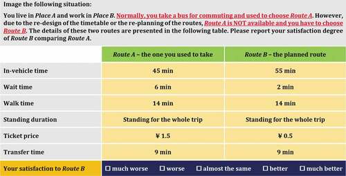
A stated choice experiment about bus line satisfaction is designed to investigate travelers’ heterogeneous loss attitudes. Stated choice experiment is adopted because it has a prominent advantage – its ability to mimic the situation that does not yet exist in the current real world (Louviere, Hensher, and Swait 2000). The context of the stated choice is commute travel. Suppose a new transport policy is introduced which leads to re-design of the timetable or certain bus lines. Two hypothetic bus lines are presented to a respondent – one acts as the bus line the respondent used to take and the other is the planned one. A respondent is firstly required to provide his/her own information (i.e. socio-demographic attributes) and then to report his/her satisfaction degree about the new bus line comparing to the old one using a 5-degree Likert scale (‘much worse’, ‘worse’, ‘almost the same’, ‘better’ and ‘much better’).

The attributes of bus lines used in the experiment along with their definitions and corresponding levels are shown in Table 1. Specifically, we separate the whole travel time into several parts: in-vehicle time, wait time, walk time and transfer time. Another attribute called ‘standing duration’ is adopted indicating whether seats are available and if not how long a respondent will stand on the bus averagely – this is an index to measure seat availability. Since standing time cannot exceed in-vehicle time, their ratio (standing time over in-vehicle time) is finally adopted. Ngene (ChoiceMetrics 2014) is applied to a simultaneous orthogonal design (i.e. orthogonality is held not only across the attributes with an alternative but also across different alternatives), in which 32 profiles with 8 blocks are obtained, which means each respondent is required to complete 4 stated choice tasks. An example of such a stated choice task is shown in Figure 1.

Table 1. Attribute details of bus lines.

Attributes	Definitions	Levels
In-vehicle Time	time in a bus (min)	35, 45, 55, 65
Wait Time	time waiting for a bus, excluding the transfer time (min)	2, 6, 10, 14
Walk Time	time walking out of a bus, excluding the transfer time (min)	2, 6, 10, 14
Standing Duration	ratio of standing time over in-vehicle time in a bus	0, 0.33, 0.67, 1
Ticket Price	price of the ticket (¥)	0.5, 1, 1.5, 2
Transfer Time	time for transfer (min)	0, 3, 6, 9

Figure 1. An example of stated choice tasks (translated from Chinese).

A survey based on this design was carried out in Dalian, China, in December 2016. Four hundred and eighty questionnaires (online and onsite) were collected. After removing the questionnaires with inconsistent and incomplete answers, 446 questionnaires were deemed valid and used in the model estimation. Since each respondent completed 4 stated choice tasks in all, there were totally 1784 observations.

The characteristics of the sample are presented in Table 2. 45.07% of the respondents are male, 56.73% are single. Over half of the respondents are aged between 20 and 30 (54.71%), followed by those aged between 30 and 40 (22.20%), which are the most active groups of commuting through public transit. About half of the respondents (accounting for 43.05%) have no driving experience, which means those respondents have to take public transit for commuting. Income distribution shows that most respondents have an income under ¥7,000 per month (accounting for 75.79% totally), which is consistent with the age distribution. The education level distribution shows that most of the respondents (accounting for 90.58% totally) have at least a bachelor degree. From the summary of sample characteristics, we can conclude that the sample is almost uniformly distributed in terms of gender, marital status; most respondents are aged below 40 and well educated (bachelor degree), and have low or middle incomes (below ¥7,000 per month) and short driving experience (less than 5 years).

Table 2. Distribution of sample characteristics.

Socio-demographic attribute	Level	Percentage
Gender	Male	45.07%
	Female	54.93%
Marital Status	Single	56.73%
	Married	43.27%
Age	≤ 20	13.68%
	21 ~ 30	54.70%
	31 ~ 40	22.20%
	41 ~ 50	5.61%
	51 ~ 65	2.91%
	≥ 66	0.90%
Driving Experience (Year)	0	43.05%
	(0, 1]	15.92%
	(1, 3]	19.06%
	(3, 5]	12.11%
	(5, 10]	6.95%
	> 10	2.91%
Income (Yuan/Month)	≤ 3499	42.83%
	3500 ~ 6999	32.96%
	7000 ~ 9999	15.47%
	10,000 ~ 14,999	6.05%
	15,000 ~ 19,999	2.02%
	≥ 20,000	0.67%
Education Level	High school or lower	9.42%
	Bachelor	76.23%
	Master/PhD	14.35%

Estimation results and analysis

Estimation results – synthetic data

The proposed model (hereafter labeled as loss-attitude model) is compared with a conventional ordered logit model (hereafter labeled as base model). Note that the loss-attitude model could be reduced to the base model by fixing all loss-attitude parameters to 1 (i.e. ${\lambda }_m=1,\mathrm{\forall }m$). To this end, two synthetic data sets¹ are generated according to the loss-attitude model and the base model, respectively, which are labeled as loss-attitude data and base data, correspondingly. The procedure of generating these synthetic data sets is presented as follows. Firstly, computing the choice probability of each degree of satisfaction according to the parameter values (i.e. the target values) presented in Table 3. Secondly, a respondent’ satisfaction degree is simulated using Monte Carlo method, i.e. first randomly generating a number between 0 and 1 then comparing the random number and the choice probability of each degree of satisfaction. Third, the whole profiles are repeated 5000 times in order to guarantee for the efficiency and reliability of the estimated parameter values, which means totally 160,000 observations for each data set are generated. Note that when computing the choice probability of each degree of satisfaction, the loss-attitude parameter is represented in an exponential form as it is in Equation (8)(8) ${\lambda }_m=exp\left({\lambda }_{m0}+\sum _l{\lambda }_{ml}{z}_l+{\xi }_m\right),{\xi }_m\sim N\left(0,{\sigma }_m\right)$(8) and only a constant is involved – this is because the synthetic data sets are adopted to examine the loss-attitude model’s ability of capturing the effect of loss attitudes rather than to investigate the composition of this effect, which is the emphasis of the next sub-section.

Table 3. The parameter values to generate synthetic data.

	Data 0	Data 1
Alternative-specific attributes
In-vehicle time	−2.6	−2.6
Wait time	−3.2	−3.2
Walk time	−2.2	−2.2
Standing duration	−0.8	−0.8
Ticket price	−0.4	−0.4
Transfer time	−3.6	−3.6
Loss attitude parameters (exponential form)
In-vehicle time	0.0	−0.2
Wait time	0.0	−0.2
Walk time	0.0	0.0
Standing duration	0.0	0.0
Ticket price	0.0	0.2
Transfer time	0.0	0.2
Threshold 1	−2.5	−2.5
Threshold 2	−1.2	−1.2
Threshold 3	−0.2	−0.2
Threshold 4	1.6	1.6

The loss-attitude model was estimated using both data sets. So does the base model. All attributes of a bus line entered the models continuously. Table 4 presents the estimation results. The final log-likelihood and root-mean-square (RMSE) are adopted to compare the model performances and the estimated parameters are also tested to examine whether they are statistically different from the corresponding target values. The RMSE is computed using Equation (11)(11) $RMSE=\sqrt{{\sum }_{n=1}^N{\left({\hat{\gamma }}_n-{\gamma }_n\right)}^2/N}$(11) , in which ${\hat{\gamma }}_n$ is the estimated value for a certain parameter, ${\gamma }_n$ is the corresponding target value and $N$ is the number of parameters to be compared in all.

(11) $RMSE=\sqrt{{\sum }_{n=1}^N{\left({\hat{\gamma }}_n-{\gamma }_n\right)}^2/N}$(11)

Table 4. Estimation results based on synthetic data (t values in the parenthesis).

	base data | base model	base data | loss-attitude model	loss-attitude data | base model	loss-attitude data | loss-attitude model
Alternative-specific attributes
In-vehicle time	-2.6396	-2.6271	-2.3866	-2.6361
	(-2.1725)	(-0.7033)	(11.8488)	(-0.9362)
Wait time	-3.1764	-3.2775	-2.8720	-3.2622
	(0.5388)	(-0.8030)	(7.5233)	(-0.6448)
Walk time	-2.2283	-2.1502	-2.2320	-2.1313
	(-0.6524)	(0.5959)	(-0.7400)	(0.8224)
Standing duration	-0.7924	-0.7841	-0.8030	-0.7854
	(0.8617)	(0.8560)	(-0.3434)	(0.7824)
Ticket price	-0.3952	-0.4040	-0.4438	-0.4035
	(0.8305)	(-0.3396)	(-7.5211)	(-0.2993)
Transfer time	-3.5863	-3.6409	-3.7713	-3.6119
	(0.2364)	(-0.3177)	(-2.9660)	(-0.0922)
Loss attitude parameters (exponential form)
In-vehicle time	0 (fixed)	0.0124	0 (fixed)	-0.1881
		(0.5391)		(0.4697)
Wait time	0 (fixed)	-0.0689	0 (fixed)	-0.2643
		(-1.3147)		(-1.1004)
Walk time	0 (fixed)	0.0734	0 (fixed)	0.0878
		(1.1454)		(1.3672)
Standing duration	0 (fixed)	0.0244	0 (fixed)	0.0309
		(0.6013)		(0.7679)
Ticket price	0 (fixed)	-0.0418	0 (fixed)	0.1571
		(-0.8104)		(-0.9149)
Transfer time	0 (fixed)	-0.0310	0 (fixed)	0.1803
		(-0.5080)		(-0.3542)
Threshold 1	-2.4951	-2.4920	-2.5188	-2.4971
	(0.5499)	(0.4763)	(-2.0933)	(0.1693)
Threshold 2	-1.1934	-1.1897	-1.2098	-1.1891
	(1.0709)	(0.6684)	(-1.5801)	(0.7100)
Threshold 3	-0.1989	-0.1951	-0.2182	-0.1976
	(0.1965)	(0.3255)	(-3.3652)	(0.1583)
Threshold 4	1.5978	1.6011	1.5755	1.5982
	(-0.3303)	(0.0710)	(-3.6341)	(-0.1148)
Convergent LL	-225444.9	-225442.6	-226129.9	-226080.5
RMSE	0.014277	0.039498	0.147223	0.039979

Note: the t values are to test if an estimated value is statistically different from its target value

Note: the column name ‘X data – Y model’ means the results in this column are from estimating Y model using X data

From Table 4, some conclusions can be made. Firstly, when the synthetic data reveal neutral loss attitude (i.e. neither loss aversion nor loss unconcern), the base model is just slightly better than the loss-attitude model in terms of RMSE and their final log-likelihoods are almost the same given their absolute values. In addition, the results of the base model show the estimated value of in-vehicle time is significantly different from its target value while the results of loss-attitude model do not show this phenomenon at all – see the second and third columns in Table 4. Secondly, when the synthetic data do reveal heterogeneous loss attitudes, the loss-attitude model outperforms the base model in term of the final log-likelihood and RMSE. Meanwhile, results show the base model cannot restore the target values since most estimated values are significantly different from the target values. However, this does not appear in the results of the loss-attitude model – see the last two columns in Table 4.

To sum up, the loss-attitude model could capture travelers’ heterogeneous loss attitudes; even no loss aversion or loss unconcern are revealed, the loss-attitude model can still capture travelers’ preferences and its performance is at least as good as the base model, which does not considering any effects of loss attitudes. However, if travelers do reveal heterogeneous loss attitudes, the base model cannot capture such effects and would generate bias in travelers’ preferences toward the alternative-specific attributes.

Estimation results – empirical data

Now the empirical data set is adopted to investigate the composition of travelers’ loss attitudes. All attributes of a bus line entered the models continuously while the socio-demographic attributes entering the loss-attitude parameters were effects coded (Hensher, Rose, and Greene 2015). In the pretest results, we found that the estimated values of taste parameters toward in-vehicle time, wait time, walk time and transfer time are too small, therefore we finally decided to shift their unit from ‘minute’ to ‘hour’. In addition, we also found that the loss-attitude parameters toward wait time, walk time, ticket price and transfer time were not significant. Therefore, in the final results these loss-attitude parameters ${\lambda }_m$ were fixed to 1. Besides, in the composition of loss attitudes toward in-vehicle time and standing duration, all insignificant attributes were also removed from the final results.

The two models were estimated using package ‘maxLik’ (Henningsen and Toomet 2011) in R, and scrambled Halton sequences (Braaten and Weller 1979) were adopted in order to simulate the distributions of random error terms in loss-attitude parameters. The reason that Halton sequences rather than pseudo-random sequences were used is that Halton sequences could mimic a certain distribution with much less draws, and scrambled Halton sequences have another advantage that the independence of different sequences is guaranteed (Bhat 2003). However, even with (scrambled) Halton sequences, it was still found that different number of draws may lead to different results (Train 2009). Therefore, to investigate the influence of different numbers of scrambled Halton draws on the estimation results, the loss-attitude model was estimated several times based on different numbers of draws, from 100 to 1,000 with step size 100. The final log-likelihoods are shown in Figure 2. Figure 2 shows that the largest difference among those final log-likelihoods is less than 0.5, which confirms that the estimation results are quite stable in spite of the different number of scrambled Halton draws. Meanwhile, with the increasing of the number of scrambled Halton draws, the final log-likelihood tends to be more stable. Therefore, in this study we present the estimation results with the number of scrambled Halton draws $R=1,000$.

Figure 2. Final log-likelihoods based on various numbers of scrambled Halton draws.

Table 5 and Table 6 show the estimation results for the base model and the loss-attitude model, respectively. Results show that both models have acceptable goodness of fit. The loss-attitude model is just slightly better than the base model in terms of the adjusted Rho-squared index. Meanwhile, the corresponding taste parameters from two models are inconsistent – given the conclusions from last sub-section, we believe there are greater estimated bias in the results of the base model. In addition, since these two models are nested, likelihood ratio test, which states that twice the difference of two nested models’ final log-likelihoods is an estimated Chi-squared statistic with degree of freedom equals the difference of parameter numbers of the two models (Hensher, Rose, and Greene 2015), could be applied to test whether the loss-attitude model statistically outperforms the base model. The log-likelihoods for these two models are −2,537.777 and −2,516.739, respectively, and the 99% critical value of the estimated Chi-squared statistic with degree of freedom equals 6 is 16.812 – the estimated Chi-squared statistic (i.e. 42.076) exceeds the critical value, which means statistically the loss-attitude model does have better performance. We further compute the utilities contributed by changes of in-vehicle time and standing duration using the estimated taste parameters and the means of estimated loss-attitude parameters. The results are presented in Figures 3 and 4, which clearly reveal the asymmetric responses to changes of gains and losses. Specifically, the loss-attitude model shows that less utility (more disutility) would be generated if respondents are confronted with changes of gains (losses) – this phenomenon is more significant to in-vehicle time than to standing duration. The means of loss-attitude parameters² to in-vehicle time and standing duration are 3.2437 and 1.4395, respectively, which indicates that averagely respondents reveal loss aversion as most previous studies found.

Table 5. Estimation results for the base model.

	Estimate	Std. Error	p-value
Alternative-specific attributes
In-vehicle time	−2.6156	0.1677	0.0000 ***
Wait time	−3.2072	0.4152	0.0000 ***
Walk time	−2.2040	0.4178	0.0000 ***
Standing duration	−0.8028	0.0804	0.0000 ***
Ticket price	−0.3700	0.0534	0.0000 ***
Transfer time	−3.5556	0.5281	0.0000 ***
Threshold 1	−2.4581	0.0866	0.0000 ***
Threshold 2	−1.2491	0.0621	0.0000 ***
Threshold 3	0.1685	0.0498	0.0007 ***
Threshold 4	1.6398	0.0642	0.0000 ***
Initial log-likelihood	−2871.237
Final log-likelihood	−2537.777
Rho-squared	0.1161
Adjusted Rho-squared	0.1127
Number of parameters	10
Number of observations	1784

*** p-value <0.01; ** p-value <0.05; * p-value <0.1

Table 6. Estimation results for the loss-attitude model.

	Estimate	Std. Error	p-value
Alternative-specific attributes
In-vehicle time	−1.3585	0.3611	0.0002 ***
Wait time	−3.3398	0.4467	0.0000 ***
Walk time	−2.3214	0.4448	0.0000 ***
Standing duration	−0.7686	0.1072	0.0000 ***
Ticket price	−0.4015	0.0570	0.0000 ***
Transfer time	−3.2457	0.6000	0.0000 ***
Threshold 1	−3.0652	0.1830	0.0000 ***
Threshold 2	−1.6503	0.1120	0.0000 ***
Threshold 3	−0.1280	0.0836	0.1258
Threshold 4	1.3788	0.0897	0.0000 ***
Loss attitude to in-vehicle time^†
Constant	0.9480	0.3323	0.0043 ***
std. deviation	0.6764	0.1774	0.0001 ***
Income (Yuan/Month)
≥ 7000	0.3810	(referenced level)
≤ 3499	−0.2719	0.1130	0.0162 **
3500 ~ 6999	−0.1091	0.0997	0.2741
Marital status
Married	−0.2203	(referenced level)
Single	0.2052	0.0847	0.0154 **
Loss attitude to standing duration
std. deviation	−0.8536	0.2739	0.0018 ***
Initial log-likelihood	−2871.237
Final log-likelihood	−2516.739
Rho-squared	0.1235
Adjusted Rho-squared	0.1179
Number of parameters	16
Number of scrambled Halton draws	1000
Number of observations	1784

*** p-value <0.01; ** p-value <0.05; * p-value <0.1

^†All socio-demographic attributes are effects coded

Figure 3. Changes in attribute utility in terms of in-vehicle time.

Figure 4. Changes in attribute utility in terms of standing duration.

Analysis of heterogeneous loss attitudes

The results reveal that respondents’ do not show any significant loss aversion or loss unconcern toward wait time, walk time, transfer time and ticket price. Meanwhile, the results also show respondents have various loss attitudes toward in-vehicle time and standing duration. Interestingly, no evidence supports any effects of loss aversion or loss unconcern to the only monetary attribute – ticket price. It is a remarkable difference from conclusions in economics. However, in transportation domain, some studies have already found that the magnitude of loss aversion effect in time dimension is larger than it is in cost dimension (e.g. Hjorth and Fosgerau 2009).

In terms of the contributions of respondents’ socio-demographic attributes to their loss attitudes, results show income and marital status are significant to the loss attitude in terms of in-vehicle time while none of them are significant in terms of standing duration. Specifically, respondents who are married and have a low income (≤ ¥6,999 per month) reveal weaker effects of loss aversion toward in-vehicle time. The conclusion about income is straightforward – those with higher incomes may have higher values of time which makes them more sensitive to changes of losses. The conclusion about marital status is surprising because we have believed getting married means more responsibility which may lead to a stronger effect of loss aversion. To sum up, the relationship between socio-demographic attributes and the travelers’ loss attitude is not as significant as we have expected.

Since loss-attitude parameter ${\lambda }_m$ is assumed to be log-normally distributed, its 95% confidence intervals can be computed³: [0.8483, 7.8499] for in-vehicle time and [0.2456, 4.0714] for standing duration. The results firstly show that the effect of loss attitude distributes wider in terms of in-vehicle time than it does in terms of standing duration and secondly support our argument that some respondents may reveal loss unconcern (i.e. the loss-attitude parameter ${\lambda }_m$ falls between 0 and 1) rather than loss aversion. Specifically, 8.05% and 50.00% (i.e. the probability of loss-attitude parameter ${\lambda }_m$ falling between 0 and 1) in the sample show loss unconcern toward in-vehicle time and standing duration, respectively. The majority of previous studies assume the existence of loss aversion effect in advance; however, our results indicate such assumption may cause bias when adopting the estimation results to further analysis.

Analysis of WTP and WTA involving loss attitude

The asymmetric responses to changes of gains and losses make respondents’ willingness-to-pay (WTP) and willingness-to-accept (WTA) also asymmetric. Figure 5 show respondents’ response to changes of gains (i.e. WTP) in terms of in-vehicle time as well as different responses to changes of losses (i.e. WTA) with the loss-attitude parameter ${\lambda }_m$ taking the lower/upper bound of 95% confidence interval, 1 and the mean (see the values in the parentheses in legend), respectively. Figure 6 shows the responses in terms of standing duration. Note that response to losses with loss-attitude parameter ${\lambda }_m$ being 1 (i.e. neutral loss attitude) is just a mirror of response to gains. In detail, respondents would like to pay at most extra ¥3.4 (1.3585/0.4015)⁴ to save 1 h of in-vehicle time and at most pay extra ¥1.9 (0.7686/0.4015) to escape from standing in the bus. However, to WTA, the situations are totally different. If the in-vehicle time is increased by an extra 1 h, respondents would like to accept at least from ¥2.9 (0.8483 × 1.3585/0.4015) to ¥25.3 (7.8499 × 1.3585/0.4015) based on the various loss attitudes; if there are no seats available in the bus for the whole trip, respondents would like to accept at least from ¥0.5 (0.2456 × 0.7686/0.4015) to ¥7.8 (4.0714 × 0.7686/0.4015) based on travelers’ various loss attitudes.

Figure 5. Responses to gains and losses in terms of in-vehicle time.

Figure 6. Responses to gains and losses in terms of standing duration.

To policy-makers, these results remind them to pay attention to respondents’ heterogeneous loss attitudes when analyzing the WTA/WTP. Missing either the effect of loss attitude or its heterogeneity property would lead to significant monetary loss. In addition, these results also remind the policy-makers to deal with attributes with higher importance first. In our case, the policy-makers should first keep an eye on in-vehicle time since respondents are more sensitive to this attribute and improvements in this attribute would get more benefits.

Discussion and conclusions

The loss-attitude effect on consumers’ choice behavior has been analyzed in economics for several decades. However, such studies in transportation domain have only appeared since the beginning of this century. Some of its properties are still unclear to transportation researchers. This study focuses on its heterogeneity property and three assumptions are made: 1) travelers’ loss attitudes are attribute-specific, 2) travelers’ loss attitudes are related to their socio-demographic attributes and 3) some travelers may show loss unconcern rather than loss aversion. To test our assumptions, an advanced ordered logit model involving heterogeneous loss-attitude effects was proposed. Specifically, attribute-specific loss attribute parameters were defined as a function of travelers’ socio-demographic attributes and assumed to be log-normally distributed. A stated preference experiment was designed and both synthetic data and empirical data based on the experiment were used for model estimation. The estimation results from synthetic data prove the ability of the proposed model to capture the effect of loss attitude and the results from empirical data confirm all of our assumptions: 1) heterogeneous effects of travelers’ loss attitudes are found only to in-vehicle time and standing duration; no evidence shows significant effect to the monetary attribute (i.e. ticket price) – which is always the only attribute considered in most economic studies; 2) travelers’ socio-demographic attributes have significant but only slightly contributions to the composition of travelers’ loss attitudes; 3) generally travelers display loss aversion but they may also display the reverse of loss aversion, i.e. loss unconcern as well – to our best knowledge, this is the first time in transportation domain to discuss and examine this effect in detail.

Although we have found evidences of travelers’ heterogeneous loss attitudes, this study still suffers from some shortcomings. First of all, a one-wave stated choice experiment is adopted, in which the alternative that respondents used to take is designed rather than offered by respondents themselves. A better approach is using two-wave choice experiments. Second, the contributions of socio-demographic attributes to the composition of loss attitudes are not as significant as we have expected. On the one hand, it may lie in the factor that the sample in this study is uneven distributed in terms of some socio-demographic attributes (e.g. education level), which actually results from a disadvantage of stated preference experiment that it cannot easily represent personal constraints effectively (Louviere, Hensher, and Swait 2000). On the other hand, this conclusion is still imaginable, after all loss attitude is in fact unobserved which may be rooted in travelers’ personalities. Therefore, further studies could involve some latent factors and a hybrid choice model may be a good way to do so. Third, this study takes bus line satisfaction as an example to investigate the proposed assumptions of heterogeneity of loss attitudes, we expect more empirical studies in different cases in the future.

Disclosure statement

No potential conflict of interest was reported by the authors.

Notes

1. The choice context is bus line satisfaction, the profiles generated for the stated choice experiment are adopted. The unit of in-vehicle time, wait time, walk time and transfer time are shifted from ‘minute’ to ‘hour’.

2. Because we use an exponential form to represent loss-attitude parameter, see Equation (8)(8) ${\lambda }_m=exp\left({\lambda }_{m0}+\sum _l{\lambda }_{ml}{z}_l+{\xi }_m\right),{\xi }_m\sim N\left(0,{\sigma }_m\right)$(8) , the mean of loss-attitude parameter equals $exp\left({\lambda }_{m0}+{{\sigma }_m}^2/2\right)$. Since socio-demographic attributes are effects coded, they are not considered when we talking about the average value.

3. Socio-demographic attributes also not considered here.

4. Note that there is no loss aversion nor loss unconcern effects in terms of ticket price.

References

- Abdellaoui, M., H. Bleichrodt, and C. Paraschiv. 2007. “Loss Aversion under Prospect Theory: A Parameter-Free Measurement.” Management Science 53 (10): 1659–1674. doi:10.1287/mnsc.1070.0711.
- Bekhor, S., C. G. Chorus, and T. Toledo. 2012. “Stochastic User Equilibrium for Route Choice Model Based on Random Regret Minimization.” Transportation Research Record 2284: 100–108. doi:10.3141/2284-12.
- Ben-Akiva, M., D. McFadden, K. E. Train, J. L. Walker, C. R. Bhat, M. Bierlaire, D. Bolduc et al. 2002. “Hybrid Choice Models: Progress and Challenges.” Marketing Letters 13 (3): 163–175. DOI:10.1023/A:1020254301302.
- Ben-Akiva, M., and S. R. Lerman. 1985. Discrete Choice Analysis: Theory and Application to Travel Demand. MIT Press, Cambridge, USA.
- Bhat, C. R. 2003. “Simulation Estimation of Mixed Discrete Choice Models Using Randomized and Scrambled Halton Sequences.” Transportation Research Part B: Methodological 37 (9): 837–855. doi:10.1016/S0191-2615(02)00090-5.
- Braaten, E., and G. Weller. 1979. “An Improved Low-Discrepancy Sequence for Multidimensional Quasi-Monte Carlo Integration.” Journal of Computational Physics 33 (2): 249–258. doi:10.1016/0021-9991(79)90019-6.
- ChoiceMetrics. 2014. Ngene 1.1.2 User Manual & Reference Guide: The Cutting Edge in Experimental Design, www.choice-metrics.com .
- Chorus, C. G. 2010. “A New Model of Random Regret Minimization.” European Journal of Transport and Infrastructure Research 10 (2): 181–196.
- Chorus, C. G. 2014. “A Generalized Random Regret Minimization Model.” Transportation Research Part B: Methodological 68: 224–238. doi:10.1016/j.trb.2014.06.009.
- Chorus, C. G., T. A. Arentze, and J. P. T. Harry. 2008. “A Random Regret-Minimization Model of Travel Choice.” Transportation Research Part B: Methodological 42 (1): 1–18. doi:10.1016/j.trb.2007.05.004.
- Connors, R. D., and A. Sumalee. 2009. “A Network Equilibrium Model with Travellers’ Perception of Stochastic Travel Times.” Transportation Research Part B: Methodological 43 (6): 614–624. doi:10.1016/j.trb.2008.12.002.
- Cranenburgh, S. V., C. A. Guevara, and C. G. Chorus. 2015. “New Insights on Random Regret Minimization Models.” Transportation Research Part A: Policy and Practice 74: 91–109.
- Engelhardt, G. V. 2003. “Nominal Loss Aversion, Housing Equity Constraints, and Household Mobility: Evidence from the United States.” Journal of Urban Economics 53 (1): 171–195. doi:10.1016/S0094-1190(02)00511-9.
- Feo-Valero, M., A. I. Arencibia, and R. Concepción. 2016. “Analyzing Discrepancies between Willingness to Pay and Willingness to Accept for Freight Transport Attributes.” Transportation Research Part E: Logistics and Transportation Review 89: 151–164. doi:10.1016/j.tre.2016.03.004.
- Genesove, D., and C. Mayer. 2001. “Loss Aversion and Seller Behavior: Evidence from the Housing Market.” The Quarterly Journal of Economics 116 (4): 1233–1260. doi:10.1162/003355301753265561.
- Hardie, B. G. S., E. J. Johnson, and P. S. Fader. 1993. “Modeling Loss Aversion and Reference Dependence Effects on Brand Choice.” Marketing Science 12 (4): 378–394. doi:10.1287/mksc.12.4.378.
- Henningsen, A., and O. Toomet. 2011. “MaxLik: A Package for Maximum Likelihood Estimation in R.” Computational Statistics 26 (3): 443–458. doi:10.1007/s00180-010-0217-1.
- Hensher, D. A., J. M. Rose, and W. H. Greene. 2015. Applied Choice Analysis. 2nd ed. Cambridge University Press, Cambridge, UK.
- Hess, S., J. M. Rose, and D. A. Hensher. 2008. “Asymmetric Preference Formation in Willingness to Pay Estimates in Discrete Choice Models.” Transportation Research Part E: Logistics and Transportation Review 44 (5): 847–863. doi:10.1016/j.tre.2007.06.002.
- Hjorth, K. 2009. “Determinants Of The Degree Of Loss Aversion.” In Paper Selected for Presentation at The International Choice Modelling Conference 1.
- Jang, S., S. Rasouli, and J. P. T. Harry. 2017. “Incorporating Psycho-Physical Mapping into Random Regret Choice Models: Model Specifications and Empirical Performance Assessments.” Transportation 44 (5): 999–1019. doi:10.1007/s11116-016-9691-9.
- Johnson, E. J., S. Gächter, and A. Herrmann. 2006. “Exploring the Nature of Loss Aversion.” IZA Discussion Paper No. 2015.
- Kahneman, D., and A. Tversky. 1979. “Prospect Theory: An Analysis of Decision under Risk.” Econometrica 47 (2): 263–292. doi:10.2307/1914185.
- Kim, J., S. Rasouli, and J. P. T. Harry. 2014. “Hybrid Choice Models: Principles and Recent Progress Incorporating Social Influence and Nonlinear Utility Functions.” Procedia Environmental Sciences 22: 20–34. doi:10.1016/j.proenv.2014.11.003.
- Louviere, J. J., D. A. Hensher, and J. Swait. 2000. Stated Choice Methods: Analysis and Applications. Cambridge University Press, Cambridge, UK.
- Masiero, L., and D. A. Hensher. 2010. “Analyzing Loss Aversion and Diminishing Sensitivity in a Freight Transport Stated Choice Experiment.” Transportation Research Part A: Policy and Practice 44 (5): 349–358.
- Nicolau, J. L. 2011. “Differentiated Price Loss Aversion in Destination Choice: The Effect of Tourists’ Cultural Interest.” Tourism Management 32 (5): 1186–1195. doi:10.1016/j.tourman.2010.11.002.
- Nicolau, J. L. 2012. “Asymmetric Tourist Response to Price: Loss Aversion Segmentation.” Journal of Travel Research 51 (5): 568–576. doi:10.1177/0047287511431321.
- Novemsky, N., and D. Kahneman. 2005. “The Boundaries of Loss Aversion.” Journal of Marketing Research 42 (2): 119–128. doi:10.1509/jmkr.42.2.119.62292.
- Prato, C. G. 2014. “Expanding the Applicability of Random Regret Minimization for Route Choice Analysis.” Transportation 41 (2): 351–375. doi:10.1007/s11116-013-9489-y.
- Rasouli, S., and J. P. T. Harry. 2017. “Specification of Regret-Based Models of Choice Behaviour: Formal Analyses and Experimental Design Based Evidence.” Transportation 44 (6): 1555–1576. doi:10.1007/s11116-016-9714-6.
- Schwanen, T., and D. Ettema. 2009. “Coping with Unreliable Transportation When Collecting Children: Examining Parents’ Behavior with Cumulative Prospect Theory.” Transportation Research Part A: Policy and Practice 43 (5): 511–525.
- Train, K. E. 2009. Discrete Choice Methods with Simulation. 2nd ed. Cambridge University Press, Cambridge, UK.
- Tversky, A., and D. Kahneman. 1992. “Advances in Prospect Theory: Cumulative Representation of Uncertainty.” Journal of Risk and Uncertainty 5 (4): 297–323. doi:10.1007/BF00122574.
- Xu, H., Y. Lou, Y. Yin, and J. Zhou. 2011. “A Prospect-Based User Equilibrium Model with Endogenous Reference Points and Its Application in Congestion Pricing.” Transportation Research Part B: Methodological 45 (2): 311–328. doi:10.1016/j.trb.2010.09.003.